TI-Basic Developer
1 propzint

| Command Summary | Command Syntax | Calculator Compatibility | Token Size |
|---|---|---|---|
| Computes a Z confidence interval of a proportion. | 1-PropZInt(x, n[, confidence level]) | TI-83/84/+/SE | 2 bytes |
Menu Location
When editing a program, press:
1. STAT to access the statistics menu
2. LEFT to access the TESTS submenu
3. ALPHA A to select 1-PropZInt(, or use arrows
(this key sequence will give you the 1-PropZInt... screen outside a program)
The 1-PropZInt( Command
The 1-PropZInt( command calculates a confidence interval for a proportion, at a specific confidence level: for example, if the confidence level is 95%, you are 95% certain that the proportion lies within the interval you get. The command assumes that the sample is large enough that the normal approximation to binomial distributions is valid: this is true if, in the sample you take, the positive and negative counts are both >5.
The 1-PropZInt( command takes 3 arguments. The first, x, is the positive count in the sample. The second, n, is the total size of the sample. (So the sample proportion is equal to x out of n). The third argument is the confidence level, which defaults to 95.
The output gives you a confidence interval of the form (a,b), meaning that the true proportion π is most likely in the range a<π<b, and the value of x/n.
Sample Problem
You want to know the proportion of students at your school that support a particular political candidate. You take a random sample of 50 students, and find that 22 of them support that candidate. 22, the positive count, and 50-22=28, the negative count, are both >5, so the assumption is satisfied.
Using 22 for x, and 50 for n, you decide to find a 95% confidence interval. The syntax for that is:
:1-PropZInt(22,50,95
which can also be
:1-PropZInt(22,50,.95
The output if you run the above code will look approximately like this:
1-PropZInt
(.30241,.57759)
p=.44
n=50
This tells you that between about 30.2% and about 57.8% of the students at your school are in support of the political candidate.
Optimization
If the confidence level is 95%, you can omit the final 95, since that is the default value:
:1-PropZInt(22,50,95
can be
:1-PropZInt(22,50
Error Conditions
- ERR:DOMAIN is thrown if the sample proportion is not between 0 and 1, any argument is negative, or the confidence level is 100 or more.
Related Commands
1 propztest

| Command Summary | Command Syntax | Calculator Compatibility | Token Size |
|---|---|---|---|
| Performs a z-test on a proportion. | 1-PropZTest(p0, x, n[, alternative, draw?] ) | TI-83/84/+/SE | 2 bytes |
Menu Location
While editing a program, press:
1. STAT to access the statistics menu
2. LEFT to access the TESTS submenu
3. 5 to select 1-PropZTest, or use arrows
(outside the program editor, this will select the 1-PropZTest... interactive solver)
The 1-PropZTest( Command
1-PropZTest performs an z-test to compare a population proportion to a hypothesis value. This test is valid for sufficiently large samples: only when the number of successes (x in the command syntax) and the number of failures (n-x) are both >5.
The logic behind the test is as follows: we want to test the hypothesis that the true proportion is equal to some value p0 (the null hypothesis). To do this, we assume that this "null hypothesis" is true, and calculate the probability that the (usually, somewhat different) actual proportion occurred, under this assumption. If this probability is sufficiently low (usually, 5% is the cutoff point), we conclude that since it's so unlikely that the data could have occurred under the null hypothesis, the null hypothesis must be false, and therefore the true proportion is not equal to p0. If, on the other hand, the probability is not too low, we conclude that the data may well have occurred under the null hypothesis, and therefore there's no reason to reject it.
Commonly used notation has the letter π being used for the true population proportion (making the null hypothesis be π=p0). TI must have been afraid that this would be confused with the real number π, so on the calculator, "prop" is used everywhere instead.
In addition to the null hypothesis, we must have an alternative hypothesis as well - usually this is simply that the proportion is not equal to p0. However, in certain cases, our alternative hypothesis may be that the proportion is greater or less than p0.
The arguments to 1-PropZTest( are as follows:
- p0 - the value for the null hypothesis (the proportion you're testing for)
- x - the success count in the sample
- n - the total size of the sample (so the sample proportion would be x/n)
- alternative (optional if you don't include draw?) - determines the alternative hypothesis
- 0 (default value) - prop≠p0
- -1 (or any negative value) - prop
- draw? (optional) set this to 1 if you want a graphical rather than numeric result
Although you can access the 1-PropZTest command on the home screen, via the catalog, there's no need: the 1-PropZTest... interactive solver, found in the statistics menu, is much more intuitive to use - you don't have to memorize the syntax.
In either case, it's important to understand the output of 1-PropZTest. Here are the meanings of each line:
- The first line, involving "prop" and p0, is the alternative hypothesis.
- z is the test statistic. If the null hypothesis is true, it should be close to 0.
- p is the probability that the difference between the proportion and p0 would occur if the null hypothesis is true. When the value is sufficiently small, we reject the null hypothesis and conclude that the alternative hypothesis is true. You should have a cutoff value ready, such as 5% or 1%. If p is lower, you "reject the null hypothesis on a 5% (or 1%) level" in technical terms.
- p-hat is the sample proportion, x/n.
- n is the sample size.
Advanced Uses
The final optional argument of 1-PropZTest, draw?, will display the results in a graphical manner if you put in "1" for it. The calculator will draw the standard normal distribution, and shade the area of the graph that corresponds to the probability p. In addition, the value of z and the value of p will be displayed. You would make your conclusions in the same way as for the regular output.
Optimization
Some of the arguments of the 1-PropZTest command have default values, and the argument can be omitted if this value is used.
- The draw? argument can be omitted if you don't want graphical output, although you could put "0" in as well.
- If the above argument is omitted, and you're doing a two sided test, you may omit the alternative argument.
Example:
:1-PropZTest(.5,22,50,0,0
can be
:1-PropZTest(.5,22,50
Error Conditions
- ERR:DOMAIN is thrown if p0 or x/n are not between 0 and 1, or x is negative or greater than n (however, any real value for alternative and draw? will work)
Related Commands
1 var stats

| Command Summary | Command Syntax | Calculator Compatibility | Token Size |
|---|---|---|---|
| Calculates some statistics for a single list of data, and stores them to statistical variables. They're also displayed in a scrollable list, if done outside a program. | 1-Var Stats [list, [freqlist]] | TI-83/84/+/SE | 1 byte |
Menu Location
Press:
1. STAT to access the statistics menu
2. LEFT to access the CALC submenu
3. 1 or ENTER to select 1-Var Stats
The 1-Var Stats Command
This command calculates a bunch of common (and a few uncommon) statistics for a list (it uses L1 by default, but you can use any list by supplying it as an argument). You have to store the list to a variable first, though, before calculating statistics for it. For example:
:{5,12,7,8,4,9→L1
:1-Var Stats
Like other statistical commands, you can use a frequency list as well, for cases where one element occurs more times than another (you can do this with a normal list, too, but that might be inconvenient when an element occurs very many times). For example:
:{1,2,3→L1
:{5,3,2→L2
:1-Var Stats L1,L2
is the frequency-list equivalent of:
:{1,1,1,1,1,2,2,2,3,3→L1
:1-Var Stats
When you're running it from the home screen, 1-Var Stats will display the statistics; this won't happen if you do it inside a program. Either way, it will also store what it calculated to the statistics variables found in VARS>Statistics... The variables 1-Var Stats affects are:
- \(\overline{\textrm{x}}\) is the mean (average) of the elements, as returned by mean(
- Σx is the sum of the elements, as returned by sum(
- Σx² is the sum of the squares of the elements
- Sx is the sample standard deviation, as returned by stdDev(
- σx is population standard deviation
- n is the number of elements in the list, as returned by dim(
- minX is the minimum value, as returned by min(
- Q1 is the first quartile
- Med is the median, as returned by median(
- Q3 is the third quartile
- maxX is the maximum value, as returned by max(
1-Var Stats will not work with "reserved" list names that the calculator uses internally. The only known such reserved list is the list RESID, and there's no reason to suspect there are any others. Ans, TblInput, and any expression which resolves to a list, are also not appropriate for this command: store all of these to a list before doing 1-Var Stats on them.
Optimization
Aside from statistical analysis, 1-Var Stats can also be used when you want to use the values it calculates more than once. This will save on size, since, for example Σx takes up less space than sum(L1), but considering how many calculations 1-Var Stats makes, it will usually be slower. Here's a short example which saves 1 byte:
:Disp "RANGE:",max(L1)-min(L1
can be
:1-Var Stats
:Disp "RANGE:",maxX-minX
Related Commands
2 propzint

| Command Summary | Command Syntax | Calculator Compatibility | Token Size |
|---|---|---|---|
| Computes a Z confidence interval of the difference between two proportions. | 2-PropZInt(x1, n1, x2, n2, [confidence level] | TI-83/84/+/SE | 2 bytes |
Menu Location
When editing a program, press:
1. STAT to access the statistics menu
2. LEFT to access the TESTS submenu
3. ALPHA B to select 2-PropZInt(, or use arrows
(this key sequence will give you the 2-PropZInt... screen outside a program)
The 2-PropZInt( Command
The 2-PropZInt( command calculates a confidence interval for the difference between two proportions, at a specific confidence level: for example, if the confidence level is 95%, you are 95% certain that the difference lies within the interval you get. The command assumes that the sample is large enough that the normal approximation to binomial distributions is valid: this is true if, in both samples involved, the positive and negative counts are both >5.
The 1-PropZInt( command takes 5 arguments. The first two, x1 and n1 are the positive count and total count in the first sample (so the estimated value of the first proportion is x1 out of n1. The next two arguments, x2 and n2, are the positive count and total count in the second sample.
The output gives you a confidence interval of the form (a,b), which is the range of values for the difference π1-π2 (where π1 and π2 are the first and second proportions respectively). If you were looking for the difference π2-π1 all you have to do is switch two sides and negate the numbers in the interval.
Sample Problem
You want to compare the proportion of students at your school and at a friend's school. that support a particular political candidate. You take a random sample of 50 students, and find that 22 of them support that candidate. Your friend took a random sample of 75 students at his school, and found that 28 supported the candidate.
The first proportion is the proportion of supporters at your school. 22 out of 50 students support the candidate, so x1=22 and n1=50.
The second proportion is the proportion of supporters at your friend's school. 28 out of 75 students support the candidate, so x2=28 and n2=75.
If you decided to do a 95% confidence interval, you would add the argument 95 after all these, so the syntax would be as follows:
:2-PropZInt(22,50,28,75,95
which can also be
:2-PropZInt(22,50,28,75,.95
The output if you run the above code will look approximately like this:
1-PropZInt
(-.1092,.24249)
p1=.44
p2=.3733333333
n1=50
n2=75
This tells you that between about the difference betwen the proportions is between about -0.11 (your school's proportion being about 0.11 less than your friend's school's proportion) to about 0.24 (your school's proportion being about 0.24 greater than your friend's school's proportion).
Optimization
If the confidence level is 95%, you can omit the final 95, since that is the default value:
:2-PropZInt(22,50,28,75,95
can be
:2-PropZInt(22,50,28,75
Error Conditions
- ERR:DOMAIN is thrown if either proportion is not between 0 and 1, or xi is negative or greater than ni, or the confidence level is negative or at least 100.
Related Commands
2 propztest

| Command Summary | Command Syntax | Calculator Compatibility | Token Size |
|---|---|---|---|
| Performs a z-test to compare two proportions. | 2-PropZTest(x1, n1, x2, n2, [alternative, draw?] | TI-83/84/+/SE | 2 bytes |
Menu Location
While editing a program, press:
1. STAT to access the statistics menu
2. LEFT to access the TESTS submenu
3. 6 to select 2-PropZTest, or use arrows
(outside the program editor, this will select the 2-PropZTest... interactive solver)
The 2-PropZTest( Command
2-PropZTest( performs az-test to compare two population proportions. This test is valid for sufficiently large samples: only when the number of successes (x in the command syntax) and the number of failures (n-x) are both >5, for both populations.
The logic behind the test is as follows: we want to test the hypothesis that the proportions are equal (the null hypothesis). To do this, we assume that this "null hypothesis" is true, and calculate the probability that the differences between the two proportions occurred, under this assumption. If this probability is sufficiently low (usually, 5% is the cutoff point), we conclude that since it's so unlikely that the data could have occurred under the null hypothesis, the null hypothesis must be false, and therefore the proportions are not equal. If, on the other hand, the probability is not too low, we conclude that the data may well have occurred under the null hypothesis, and therefore there's no reason to reject it.
Commonly used notation has the letters π1 and π2 being used for the true population proportions (making the null hypothesis be π1=π2). TI must have been afraid that this would be confused with the real number π, so on the calculator, "p1" and "p2" are used everywhere instead.
In addition to the null hypothesis, we must have an alternative hypothesis as well - usually, this is simply that the proportions are not equal. However, in certain cases, our alternative hypothesis may be that one proportion is greater or less than the other.
The arguments to 2-PropZTest( (which must be integers, or the calculator will generate a domain error) are as follows:
- x1 - the success count in the first sample
- n1 - the total size of the first sample (so the sample proportion would be x1/n1)
- x2 - the success count in the second sample
- n2 - the total size of the second sample (so the sample proportion would be x2/n2)
- alternative (optional if you don't include draw?) - determines the alternative hypothesis
- 0 (default value) - p1≠p2
- -1 (or any negative value) - p1
- draw? (optional) set this to 1 if you want a graphical rather than numeric result
Although you can access the 2-PropZTest( command on the home screen, via the catalog, there's no need: the 2-PropZTest(... interactive solver, found in the statistics menu, is much more intuitive to use - you don't have to memorize the syntax.
In either case, it's important to understand the output of 2-PropZTest(. Here are the meanings of each line:
- The first line, involving p1 and p2, is the alternative hypothesis.
- z is the test statistic. If the null hypothesis is true, it should be close to 0.
- p is the probability that the difference between the two proportions would occur if the null hypothesis is true. When the value is sufficiently small, we reject the null hypothesis and conclude that the alternative hypothesis is true. You should have a cutoff value ready, such as 5% or 1%. If p is lower, you "reject the null hypothesis on a 5% (or 1%) level" in technical terms.
- p-hat1 is the sample proportion x1/n1.
- p-hat2 is the sample proportion x2/n2.
- p-hat is the total sample proportion
- n1 is the first sample size.
- n2 is the second sample size.
Advanced Uses
The final optional argument of 2-PropZTest(, draw?, will display the results in a graphical manner if you put in "1" for it. The calculator will draw the standard normal distribution, and shade the area of the graph that corresponds to the probability p. In addition, the value of z and the value of p will be displayed. You would make your conclusions in the same way as for the regular output.
Optimization
Some of the arguments of the 2-PropZTest( command have default values, and the argument can be omitted if this value is used.
- The draw? argument can be omitted if you don't want graphical output, although you could put "0" in as well.
- If the above argument is omitted, and you're doing a two-sided test, you may omit the alternative argument.
Example:
:2-PropZTest(22,50,48,100,0,0
can be
:2-PropZTest(22,50,48,100
Error Conditions
- ERR:DOMAIN is thrown if the values of the arguments entered are not integers.
Related Commands
2 sampftest

| Command Summary | Command Syntax | Calculator Compatibility | Token Size |
|---|---|---|---|
| Performs a F-test to compare the standard deviations of two populations. | 2-SampFTest [list1, list2, frequency1, frequency2, alternative,draw?] (data list input) 2-SampFTest s1, n1, s2, n2, [alternative,draw?] (summary stats input) |
TI-83/84/+/SE | 2 bytes |
Menu Location
While editing a program, press:
1. STAT to access the statistics menu
2. LEFT to access the TESTS submenu
3. ALPHA D to select 2-SampFTest, or use arrows
Outside the program editor, this will select the 2-SampFTest... interactive solver.
Change the last keypress to ALPHA E on a TI-84+/SE with OS 2.30 or higher.
The 2-SampFTest Command
2-SampFTest performs an F-test to compare the standard deviations of two populations. This test is valid for two normally distributed populations, but is extremely sensitive to non-normality, so it should not be used unless you are certain that the populations are normal.
The logic behind the test is as follows: we want to test the hypothesis that the standard deviations of the two populations are equal (the null hypothesis). The letter σ is used for a standard deviation, so this is usually written as σ1=σ2. To do this, we assume that this "null hypothesis" is true, and calculate the probability that the difference between the two standard deviations occurred, under this assumption. If this probability is sufficiently low (usually, 5% is the cutoff point), we conclude that since it's so unlikely that the data could have occurred under the null hypothesis, the null hypothesis must be false, and therefore the deviations are not equal. If, on the other hand, the probability is not too low, we conclude that the data may well have occurred under the null hypothesis, and therefore there's no reason to reject it.
In addition to the null hypothesis, we must have an alternative hypothesis as well - usually this is simply that the two standard deviations are not equal. However, in certain cases when we have reason to suspect that one deviation is greater than the other (such as when we are trying to verify a claim that one standard deviation is greater), our alternative hypothesis may be that the first standard deviation is greater than the second (σ1>σ2) or less (σ1<σ2).
As for the 2-SampFTest command itself, there are two ways of calling it: you may give it a list of all the sample data, or the necessary statistics about the list (s1 and s2 the sample standard deviations, and n1 and n2 the sample sizes). In either case, you can indicate what the alternate hypothesis is, by a value of 0, -1, or 1 for the alternative argument. 0 indicates a two-sided hypothesis of σ1≠σ2, -1 indicates σ1<σ2, and 1 indicates μ1>μ2. (In fact, the calculator will treat any negative value as -1, and any positive value as 1).
Although you can access the 2-SampFTest command on the home screen, via the catalog, there's no need: the 2-SampFTest... interactive solver, found in the statistics menu, is much more intuitive to use - you don't have to memorize the syntax.
In either case, it's important to understand the output of 2-SampFTest. Here are the meanings of each line:
- The first line, involving σ1 and σ2, is the alternative hypothesis.
- F is the test statistic, the ratio of the standard deviations. If the null hypothesis is true, it should be close to 1.
- p is the probability that the difference between σ1 and σ2 (the two standard deviations) would occur if the null hypothesis is true. When the value is sufficiently small, we reject the null hypothesis and conclude that the alternative hypothesis is true. You should have a cutoff value ready, such as 5% or 1%. If p is lower, you "reject the null hypothesis on a 5% (or 1%) level" in technical terms.
- Sx1 and Sx2 are the two sample standard deviations.
- x-bar1 and x-bar2 are the two sample means. They aren't used in the calculation, and will only be shown with the data list syntax.
- n1 and n2 are the sample sizes.
Advanced Uses
The final optional argument of 2-SampFTest, draw?, will display the results in a graphical manner if you put in "1" for it. The calculator will draw the distribution, and shade the area of the graph that corresponds to the probability p. In addition, the value of F and the value of p will be displayed. You would make your conclusions in the same way as for the regular output.
As with most other statistical commands, you may use frequency lists in your input (when using the data list syntax). If you do, then both lists must have frequencies, and the order of the arguments would be list1, list2, frequency1, frequency2.
Optimization
Some of the arguments of the 2-SampFTest command have default values, and the argument can be omitted if this value is accepted.
- The draw? argument can be omitted if you don't want graphical output, although you could put "0" in as well.
- If the above argument is omitted, and you're doing a two sided test, you may omit the alternative argument.
- With data list input, you can always omit the frequency lists if you won't be using them.
- With data list input, if the flags that go at the end are omitted, and you're using the default lists L1 and L2, you may omit those as well.
Example:
:2-SampFTest L1,L2,0
can be
:2-SampFTest
Related Commands
2 samptint

| Command Summary | Command Syntax | Calculator Compatibility | Token Size |
|---|---|---|---|
| Using either already-calculated statistics, or two data sets, computes a T confidence interval for the difference between two sample means. | 2-SampTInt list1, list2, [frequency1], [frequency2], [confidence level, pooled] (data list input) 2-SampTInt x1, s1, n1, x2, s2, n2, [confidence level, pooled] (summary stats input) |
TI-83/84/+/SE | 2 bytes |
Menu Location
When editing a program, press:
1. STAT to access the statistics menu
2. LEFT to access the TESTS submenu
3. 0 to select 2-SampTInt, or use arrows
(this key sequence will give you the 2-SampTInt... screen outside a program)
The 2-SampTInt Command
The 2-SampTInt command uses the techniques of T Intervals to compute an interval for the difference between the means of two independent populations, at a specified confidence level. Use 2-SampTInt( when you have two independent variables to compare, and you don't know their standard deviations. The 2-SampTInt command assumes that both your variables are normally distributed, but it will work for other distributions if the sample size is large enough.
There are two ways to call this command: by supplying it with needed sample statistics (mean, standard deviation, and sample size, for both data sets), or by entering two lists and letting the calculator work the statistics out. In either case, you will need to enter the desired confidence level as well.
In the summary stats syntax, x1 and x2 the two sample means, s1 and s2 are the two sample standard deviations, and n1 and n2 the two sample sizes.
The output will contain an open interval (a, b) that is your answer: the difference between the two means will lie in this interval. Specifically, it is the second mean subtracted from the first - μ1-μ2. If you're interested in the reverse difference, just flip the signs on the interval.
Tip: don't use this command in a matched-pairs setting when you can match the two samples up by units or subjects. Instead, take the difference between the two samples in each matched pair, and use a regular TInterval.
Sample Problem
You want to compare the average height of a freshman and a senior at your school. You haven't asked everyone, but you took a random sample of 40 people from each class and found out their heights (and stored them to L1 and L2). You've decided to use a 95% confidence interval.
Based on the data list syntax for a 2-SampTInt, here is your code:
:2-SampTInt L1,L2,95
you can also use
:2-SampTInt L1,L2,.95
Alternatively, you could calculate the mean and sample size and enter those instead. The sample size in this case is 40 for both data sets; let's say the means were 57 inches and 67 inches and the standard deviations 5.2 and 7.1 inches. You now have all the needed statistics:
- x1 is the mean height of freshmen: 57 inches
- s1 is the sample standard deviation for freshmen: 5.2 inches
- n1 is the number of freshmen in the sample: 40
- x2 is the mean height of seniors: 67 inches
- s2 is the sample standard deviation for seniors: 7.1 inches
- n2 is the number of seniors in the sample: 40
This means that the code is:
:2-SampTInt 57,5.2,40,67,7.1,40,95
you can also use
:2-SampTInt 57,5.2,40,67,7.1,40,.95
Of course, the main use of the 2-SampTInt command is in a program. While you can enter the command on the home screen as well (just look in the catalog for it), it would probably be easier to select 2-SampTInt... from the STAT>TEST menu (see the sidebar), since you don't have to remember the syntax.
Advanced Uses
As with most other statistical commands, you can add frequencies to the lists (only with the data list syntax, of course); if you do, both lists must have frequencies, and the arguments go in the order first data list, second data list, first freq. list, second freq. list. Each frequency list must contain non-negative real numbers, which can't be all 0.
There is a final argument to 2-SampTInt: pooled. It can be either 0 or 1 (although any argument that isn't 0 will get treated as a 1); the default value is 0. If the value is 1, then then the variances will be pooled: that is, the calculator will assume that the variances of the two populations are equal, and use a combined form of the two standard deviations in place of each population's individual standard deviation. Set this flag if you have reason to believe that the standard deviations are equal.
Optimization
Using the data list syntax, all items are optional: the calculator will assume you want to use L1 and L2 for your data unless other lists are supplied, and that the confidence level you want is 95% unless you give another one. Using the summary stats syntax, the confidence level is also optional - again, the calculator will assume 95%. This means we can rewrite our code above in a simpler manner:
:2-SampTInt L1,L2,95
can be
:2-SampTInt
:2-SampTInt 57,5.2,40,67,7.1,40,95
can be
:2-SampTInt 57,5.2,40,67,7.1,40
Related Commands
2 sampttest

| Command Summary | Command Syntax | Calculator Compatibility | Token Size |
|---|---|---|---|
| Performs a t significance test to compare the means of two populations. | 2-SampTTest [list1, list2, frequency1, frequency2, alternative, pooled? draw?] (data list input) 2-SampTTest x1, s1, n1, x2, s2, n2, [alternative, pooled?, draw?] (summary stats input) |
TI-83/84/+/SE | 2 bytes |
Menu Location
While editing a program, press:
1. STAT to access the statistics menu
2. LEFT to access the TESTS submenu
3. 4 to select 2-SampTTest, or use arrows
(outside the program editor, this will select the 2-SampTTest... interactive solver)
The 2-SampTTest Command
2-SampTTest performs a t significance test to compare the means of two populations. This test is valid for simple random samples from populations with unknown standard deviations. In addition, either the populations must be normally distributed, or the sample sizes have to be sufficiently large (usually, greater than 10).
The logic behind the test is as follows: we want to test the hypothesis that the true means of the two populations are equal (the null hypothesis). The letter μ is used for a population mean, so this is usually written as μ1=μ2. To do this, we assume that this "null hypothesis" is true, and calculate the probability that the difference between the two means occurred, under this assumption. If this probability is sufficiently low (usually, 5% is the cutoff point), we conclude that since it's so unlikely that the data could have occurred under the null hypothesis, the null hypothesis must be false, and therefore the means are not equal. If, on the other hand, the probability is not too low, we conclude that the data may well have occurred under the null hypothesis, and therefore there's no reason to reject it.
In addition to the null hypothesis, we must have an alternative hypothesis as well - usually this is simply that the two means are not equal. However, in certain cases when we have reason to suspect that one mean is greater than the other (such as when we are trying to verify a claim that one mean is greater), our alternative hypothesis may be that the first mean is greater than the second (μ1>μ2) or less (μ1<μ2).
As for the 2-SampTTest command itself, there are two ways of calling it: you may give it a list of all the sample data, or the necessary statistics about the list (x1 and x2 are the sample means, s1 and s2 the sample standard deviations, and n1 and n2 the sample sizes). In either case, you can indicate what the alternate hypothesis is, by a value of 0, -1, or 1 for the alternative argument. 0 indicates a two-sided hypothesis of μ1≠μ2, -1 indicates μ1<μ2, and 1 indicates μ1>μ2. (In fact, the calculator will treat any negative value as -1, and any positive value as 1).
Although you can access the 2-SampTTest command on the home screen, via the catalog, there's no need: the 2-SampTTest... interactive solver, found in the statistics menu, is much more intuitive to use - you don't have to memorize the syntax.
In either case, it's important to understand the output of 2-SampTTest. Here are the meanings of each line:
- The first line, involving μ1 and μ2, is the alternative hypothesis.
- t is the test statistic, the standardized difference between the means. If the null hypothesis is true, it should be close to 0.
- p is the probability that the difference between μ1 and μ2 (the two means) would occur if the null hypothesis is true. When the value is sufficiently small, we reject the null hypothesis and conclude that the alternative hypothesis is true. You should have a cutoff value ready, such as 5% or 1%. If p is lower, you "reject the null hypothesis on a 5% (or 1%) level" in technical terms.
- x-bar1 and x-bar2 are the two sample means.
- Sx1 and Sx2 are the two sample standard deviations.
- n1 and n2 are the sample sizes.
Sample Problem
Your school claims that the average SAT score of students at the school is higher than at a rival school. You took samples of SAT scores from students at both schools (and stored them to L1 and L2).
Since the school's claim is that your school's score is higher, that will be your alternative hypothesis (μ1>μ2), which corresponds to a value of 1. The code you'd use is:
:2-SampTTest L1,L2,1
Alternatively, you could calculate the mean, standard deviation, and size of your samples, and put those into the command instead. Suppose you obtained SAT scores from 60 students at your school and 40 students at the rival school, the means were 1737 and 1623, and the standard deviation 211 and 218. Then your code is:
:2-SampTTest 1737,211,60,1623,218,40,1
You will see the following output:
2-SampTTest
μ1>μ2
z=2.594854858
p=.0056059824
x1=1737
x2=1623
Sx1=211
Sx2=218
n1=60
n2=40
The most important part of this output is "p=.0056059824". This value of p is smaller than 1% or 0.01. This is significant on the 1% level, so we reject the null hypothesis and conclude that the alternative hypothesis is true: μ1>μ2, that is, your school's average SAT score is indeed higher.
Advanced Uses
The final optional argument of 2-SampTTest, draw?, will display the results in a graphical manner if you put in "1" for it. The calculator will draw the distribution, and shade the area of the graph beyound the t statistic. In addition, the value of t and the value of p will be displayed (the value of p corresponds to the shaded area). You would make your conclusions in the same way as for the regular output.
The optional argument pooled?, if given a nonzero value, will pool the standard deviations to find a combined value which will then be used for both populations. Use this feature if you have reason to believe that the two populations have the same standard deviation.
As with most other statistical commands, you may use a frequency list in your input (when using the data list syntax). If you do, then both lists must have frequencies, and the order of the arguments would be list1, list2, frequency1, frequency2.
Optimization
Some of the arguments of the 2-SampTTest command have default values, and the argument can be omitted if this value is accepted.
- The draw? argument can be omitted if you don't want graphical output, although you could put "0" in as well.
- If the draw? argument is omitted, you can omit the pooled? argument if you do not want your standard deviations pooled.
- If both the above arguments are omitted, and you're doing a two sided test, you may omit the alternative argument.
- With data list input, you can always omit the frequency lists if you won't be using them.
- With data list input, if the flags that go at the end are omitted, and you're using the default lists L1 and L2, you may omit those as well.
The code in the sample problem above can't be optimized, because the alternative argument is 1:
:2-SampTTest L1,L2,1
However, if we were doing a two-sided test, we could omit the alternative argument as well as the lists:
:2-SampTTest L1,L2,0
can be just
:2-SampTTest
Related Commands
2 sampzint

| Command Summary | Command Syntax | Calculator Compatibility | Token Size |
|---|---|---|---|
| Using either already-calculated statistics, or two data sets, computes a Z confidence interval for the difference between two sample means. | 2-SampZInt(σ1, σ2, [list1, list2, [frequency1], [frequency2], [confidence level] (data list input) 2-SampZInt(σ1, σ2, x1, n1, x2, n2, [confidence level] (summary stats input) |
TI-83/84/+/SE | 2 bytes |
Menu Location
When editing a program, press:
1. STAT to access the statistics menu
2. LEFT to access the TESTS submenu
3. 9 to select 2-SampZInt(, or use arrows
(this key sequence will give you the 2-SampZInt... screen outside a program)
The 2-SampZInt( Command
The 2-SampZInt( command uses the techniques of Z Intervals to compute an interval for the difference between the means of two independent populations, at a specified confidence level. Use 2-SampZInt( when you have two independent variables to compare, and you already know their standard deviations. The 2-SampZInt( command assumes that both variables are distributed normally, but it will work for other distributions if the sample size is large enough.
There are two ways to call this command: by supplying it with needed sample statistics (mean and sample size, for both data sets), or by entering two lists and letting the calculator work the statistics out. In either case, you will need to enter the standard deviation and desired confidence level as well.
In the data list syntax, σ1 and σ2 are the two standard deviations.
In the summary stats syntax, σ1 and σ2 are the two standard deviations, x1 and x2 the two sample means, and n1 and n2 the two sample sizes.
The output will contain an open interval (a, b) that is your answer: the difference between the two means will lie in this interval. Specifically, it is the second mean subtracted from the first - μ1-μ2. If you're interested in the reverse difference, just flip the signs on the interval.
Tip: don't use this command in a matched-pairs setting when you can match the two samples up by units or subjects. Instead, take the difference between the two samples in each matched pair, and use a regular ZInterval.
Sample Problem
You want to compare the average height of a freshman and a senior at your school. You haven't asked everyone, but you took a random sample of 40 people from each class and found out their heights (and stored them to L1 and L2). You've read in your textbook that the standard deviation of teenagers' heights is usually 6 inches. You've decided to use a 95% confidence interval.
Based on the data list syntax for a 2-SampZInt(, here is your code:
:2-SampZInt(6,6,L1,L2,95
you can also use
:2-SampZInt(6,6,L1,L2,.95
Alternatively, you could calculate the mean and sample size and enter those instead. The sample size in this case is 40 for both data sets; let's say the means were 57 inches and 67 inches. You now have all the needed statistics:
- σ1 is the standard deviation for freshmen: 6 inches
- σ2 is the standard deviation for seniors: also 6 inches
- x1 is the mean height of freshmen: 57 inches
- n1 is the number of freshmen in the sample: 40
- x2 is the mean height of seniors: 67 inches
- n2 is the number of seniors in the sample: 40
This means that the code is:
:2-SampZInt(6,6,57,40,67,40,95
you can also use
:2-SampZInt(6,6,57,40,67,40,.95
Of course, the main use of the 2-SampZInt( command is in a program. While you can enter the command on the home screen as well (just look in the catalog for it), it would probably be easier to select 2-SampZInt... from the STAT>TEST menu (see the sidebar), since you don't have to remember the syntax.
Advanced Uses
As with most other statistical commands, you can add frequencies to the lists (only with the data list syntax, of course); if you do, both lists must have frequencies, and the arguments go in the order first data list, second data list, first freq. list, second freq. list. Each frequency list must contain non-negative real numbers, which can't be all 0.
Optimization
Using the data list syntax, all items but the standard deviations are optional: the calculator will assume you want to use L1 and L2 for your data unless other lists are supplied, and that the confidence level you want is 95% unless you give another one. Using the summary stats syntax, the confidence level is also optional - again, the calculator will assume 95%. This means we can rewrite our code above in a simpler manner:
:2-SampZInt(6,6,L1,L2,95
can be
:2-SampZInt(6,6
:2-SampZInt(6,6,57,40,67,40,95
can be
:2-SampZInt(6,6,57,40,67,40
Related Commands
2 sampztest

| Command Summary | Command Syntax | Calculator Compatibility | Token Size |
|---|---|---|---|
| Performs a z significance test to compare the means of two populations. | 2-SampZTest(σ1, σ2 [list1, list2, frequency1, frequency2, alternative, draw?] (data list input) 2-SampZTest(σ1, σ2 x1, n1, x2, n2, [alternative, draw?] (summary stats input) |
TI-83/84/+/SE | 2 bytes |
Menu Location
While editing a program, press:
1. STAT to access the statistics menu
2. LEFT to access the TESTS submenu
3. 3 to select 2-SampZTest(, or use arrows
(outside the program editor, this will select the 2-SampZTest... interactive solver)
The 2-SampZTest( Command
2-SampZTest( performs a z significance test to compare the means of two populations. This test is valid for simple random samples from populations with known standard deviations. In addition, either the populations must be normally distributed, or the sample sizes have to be sufficiently large (usually, greater than 10).
The logic behind the test is as follows: we want to test the hypothesis that the true means of the two populations are equal (the null hypothesis). The letter μ is used for a population mean, so this is usually written as μ1=μ2. To do this, we assume that this "null hypothesis" is true, and calculate the probability that the difference between the two means occurred, under this assumption. If this probability is sufficiently low (usually, 5% is the cutoff point), we conclude that since it's so unlikely that the data could have occurred under the null hypothesis, the null hypothesis must be false, and therefore the means are not equal. If, on the other hand, the probability is not too low, we conclude that the data may well have occurred under the null hypothesis, and therefore there's no reason to reject it.
In addition to the null hypothesis, we must have an alternative hypothesis as well - usually this is simply that the two means are not equal. However, in certain cases when we have reason to suspect that one mean is greater than the other (such as when we are trying to verify a claim that one mean is greater), our alternative hypothesis may be that the first mean is greater than the second (μ1>μ2) or less (μ1<μ2).
As for the 2-SampZTest( command itself, there are two ways of calling it: after giving the two standard deviations, you may give it a list of all the sample data, or the necessary statistics about the list (x1 and x2 are the sample means, and n1 and n2 are the sample sizes). In either case, you can indicate what the alternate hypothesis is, by a value of 0, -1, or 1 for the alternative argument. 0 indicates a two-sided hypothesis of μ1≠μ2, -1 indicates μ1<μ2, and 1 indicates μ1>μ2. (In fact, the calculator will treat any negative value as -1, and any positive value as 1).
Although you can access the 2-SampZTest( command on the home screen, via the catalog, there's no need: the 2-SampZTest... interactive solver, found in the statistics menu, is much more intuitive to use - you don't have to memorize the syntax.
In either case, it's important to understand the output of 2-SampZTest. Here are the meanings of each line:
- The first line, involving μ1 and μ2, is the alternative hypothesis.
- z is the test statistic, the standardized difference between the means. If the null hypothesis is true, it should be close to 0.
- p is the probability that the difference between μ1 and μ2 (the two means) would occur if the null hypothesis is true. When the value is sufficiently small, we reject the null hypothesis and conclude that the alternative hypothesis is true. You should have a cutoff value ready, such as 5% or 1%. If p is lower, you "reject the null hypothesis on a 5% (or 1%) level" in technical terms.
- x-bar1 and x-bar2 are the two sample means.
- n1 and n2 are the sample sizes.
Sample Problem
Your school claims that the average SAT score of students at the school is higher than at a rival school. You took samples of SAT scores from students at both schools (and stored them to L1 and L2). Although you didn't know the standard deviations, you decided to use the value 200 that you found online as an estimate.
You now have all the data. You're assuming σ1 and σ2 are both 200; the two data lists are L1 and L2. Since the school's claim is that your school's score is higher, that will be your alternative hypothesis (μ1>μ2), which corresponds to a value of 1. The code you'd use is:
:2-SampZTest(200,200,L1,L2,1
Alternatively, you could calculate the mean and sample size of your sample, and put those into the command instead. Suppose you obtained SAT scores from 60 students at your school and 40 students at the rival school, and that the means were 1737 and 1623. Then your code is:
:2-SampZTest(200,200,1737,60,1623,40,1
You will see the following output:
Z-Test
μ1>μ2
z=2.792418307
p=.0026158434
x1=1737
x2=1623
n1=60
n2=40
The most important part of this output is "p=.0026158434". This value of p is much smaller than 1% or 0.01. This is significant on the 1% level, so we reject the null hypothesis and conclude that the alternative hypothesis is true: μ1>μ2, that is, your school's average SAT score is indeed higher.
Advanced Uses
The final argument of 2-SampZTest(, draw?, will display the results in a graphical manner if you put in "1" for it. The calculator will draw the standard normal curve, and shade the area of the graph beyond the z statistic. In addition, the value of z and the value of p will be displayed (the value of p corresponds to the shaded area). You would make your conclusions in the same way as for the regular output.
As with most other statistical commands, you may use a frequency list in your input (when using the data list syntax). If you do, then both lists must have frequencies, and the order of the arguments would be list1, list2, frequency1, frequency2.
Optimization
Most of the arguments of the 2-SampZTest( command have default values, and the argument can be omitted if this value is accepted.
- The draw? argument can be omitted if you don't want graphical output, although you could put "0" in as well.
- If the draw? argument is omitted, you can omit the alternative argument to use a two-sided test (μ1≠μ2). If you include the draw? argument, you have to include this - otherwise there will be confusion as to what the 5th argument means.
- With data list input, you can always omit the frequency lists if you won't be using them.
- With data list input, if the draw? and alternative arguments are omitted, and your data is in L1 and L2 (and you're not using frequency lists), you may omit L1 and L2 - those are default parameters. However, if alternative or draw? is present, you have to include it, or else the syntax may be confused with the syntax for summary stats input.
The code in the sample problem above can't be optimized, because the alternative argument is 1:
:2-SampZTest(200,200,L1,L2,1
However, if we were doing a two-sided test, we could omit the alternative argument as well as the lists:
:2-SampZTest(200,200,L1,L2,0
can be
:2-SampZTest(200,200
Related Commands
2 var stats

| Command Summary | Command Syntax | Calculator Compatibility | Token Size |
|---|---|---|---|
| Calculates some common statistics for two lists of data, and stores them to statistical variables. They're also displayed in a scrollable list, if done outside a program. | 2-Var Stats [list1, list2, [freqlist]] | TI-83/84/+/SE | 1 byte |
Menu Location
Press:
1. STAT to access the statistics menu
2. LEFT to access the CALC submenu
3. 2 to select 2-Var Stats, or use arrows
The 2-Var Stats Command
This command calculates a bunch of common (and a few uncommon) statistics for a pair of lists (it uses L1 and L2 by default, but you can use any list by supplying it as an argument). You have to store the lists to variables first, though, before calculating statistics for them. For example:
:{5,12,7,8,4,9→L1
:{1,0,2,5,7,4→L2
:2-Var Stats
The calculator treats the two lists as a list of ordered pairs. Some of the statistics calculated assume that this is the case, and the two lists are the same size: an error will occur if the lists don't match.
Like other statistical commands, you can use a frequency list as well, for cases where one element occurs more times than another (you can do this with a normal list, too, but that might be inconvenient when an element occurs very many times). There is only one frequency list for both data lists, and the frequency applies to the ordered pair formed by an element taken from each list. For example:
:{1,2,3→L1
:{1,2,3→L2
:{5,3,2→L3
:2-Var Stats L1,L2,L3
is the frequency-list equivalent of:
:{1,1,1,1,1,2,2,2,3,3→L1
:{1,1,1,1,1,2,2,2,3,3→L2
:2-Var Stats
When you're running it from the home screen, 2-Var Stats will display the statistics; this won't happen if you do it inside a program. Either way, it will also store what it calculated to the statistics variables found in VARS>Statistics... The variables 2-Var Stats affects are:
- \(\definecolor{darkgreen}{rgb}{0.90,0.91,0.859}\pagecolor{darkgreen} \overline{\textrm{x}}\) is the mean (average) of the first list
- Σx is the sum of the first list
- Σx² is the sum of the squares of the first list
- Sx is the sample standard deviation of the first list
- σx is population standard deviation of the first list
- minX is the minimum element of the first list
- maxX is the maximum element of the first list
- \(\definecolor{darkgreen}{rgb}{0.90,0.91,0.859}\pagecolor{darkgreen} \overline{\textrm{y}}\) is the mean (average) of the second list
- Σy is the sum of the second list
- Σy² is the sum of the squares of the second list
- Sy is the sample standard deviation of the second list
- σy is population standard deviation of the second list
- minY is the minimum element of the second list
- maxY is the maximum element of the second list
- Σxy is the sum of products of each matching pair of elements in the lists
- n is the number of elements in both lists
2-Var Stats will not work with "reserved" list names that the calculator uses internally. The only known such reserved list is the list RESID, and there's no reason to suspect there are any others. Ans, TblInput, and any expression which resolves to a list, are also not appropriate for this command: store all of these to a list before doing 2-Var Stats on them.
Advanced uses
If you consider the two lists to be vectors, then Σxy is their dot product, and Σx² and Σy² are the squares of their norms; math done with these and other statistics can produce the shortest (but not necessarily quickest) way to calculate many vector operations.
Optimization
Aside from statistical analysis, 2-Var Stats can also be used when you want to use the values it calculates more than once. This will save on size, since, for example Σx takes up less space than sum(L1), but considering how many calculations 2-Var Stats makes, it will usually be slower.
Related Commands
2

| Command Summary | Command Syntax | Calculator Compatibility | Token Size |
|---|---|---|---|
| Raises the input to the second power. | value² | TI-83/84/+/SE | 1 byte |
Menu Location
Press [x²]
The ² Command
The ² command raises an input to the second power. It has exactly the same function as "^2", but is one byte smaller. If used on a list, it will return a list with all of the elements squared. If used on a matrix, it will return the second matrix power of the input matrix.
2²
4
{1,‾2,3}²
{1 4 9}
[[2,‾1][‾3,0]]²
[[1 ‾2]
[6 ‾3]]
Optimization
Use this command instead of ^2 in all instances.
:X^2
can be
:X²
Related Commands
3

| Command Summary | Command Syntax | Calculator Compatibility | Token Size |
|---|---|---|---|
| Raises the input to the third power. | value³ | TI-83/84/+/SE | 1 byte |
Menu Location
While editing a program, press:
1. MATH to enter the MATH menu
2. 3 or use the arrow keys to select.
The ³ Command
The ³ command raises an input to the third power. It has exactly the same function as "^3", but is one byte smaller. If used on a list, it will return a list with all of the elements cubed. If used on a matrix, it will return the third matrix power of the input matrix.
2³
8
{1,‾2,3}³
{1 ‾8 27}
[[2,‾1][‾3,0]]³
[[20 ‾7]
[‾21 6]]
Advanced Uses
One trick with ³ is to use it to save space (at the cost of speed) when using hard-coded values. For instance, use 5³ instead of 125 to save one byte.
Optimization
Use this command instead of ^3 in all instances.
:X^3
can be
:X³
Related Commands
68k 0b

| Command Summary | Command Syntax | Calculator Compatibility | Token Size |
|---|---|---|---|
| Indicates that a number is written in binary. | 0bdigits | This command works on all calculators. | 2 bytes |
Menu Location
N/A
The 0b Command
The calculator can work with numbers written in three bases: decimal (the usual), binary, and hexadecimal. The 0b command indicates that a number is written in binary:
:0b101
5
:0b100000
32
When written in binary, numbers are expressed as signed 32-bit integers, which means that only the integers between -231 and 231-1 can be expressed in binary. With other binary-related commands, numbers are simply truncated to fit in this range. Not so with 0b: if you enter more than 32 binary digits after the 0b, the result is a domain error.
Even if the calculator is in binary mode, you still have to write 0b for an integer to be interpreted as binary: binary mode only affects output. If the calculator is in decimal mode, which is the default, you have to use 68k:▶Bin to get output in binary.
Error Conditions
260 - Domain error happens when 0b is used with more than 32 binary digits after it.
Related Commands
68k 0h

| Command Summary | Command Syntax | Calculator Compatibility | Token Size |
|---|---|---|---|
| Indicates that a number is written in hexadecimal. | 0hdigits | This command works on all calculators. | 2 bytes |
Menu Location
N/A
The 0h Command
The calculator can work with numbers written in three bases: decimal (the usual), binary, and hexadecimal. The 0h command indicates that a number is written in hexadecimal:
:0h10
16
:0h2F6
758
When written in hexadecimal, numbers are expressed as signed 32-bit integers (32 bits correspond to 8 hexadecimal digits), which means that only the integers between -231 and 231-1 can be expressed in hexadecimal. With other hexadecimal-related commands, numbers are simply truncated to fit in this range. Not so with 0h: if you enter more than 8 hexadecimal digits after the 0b, the result is a domain error.
Even if the calculator is in hexadecimal mode, you still have to write 0h for an integer to be interpreted as hexadecimal: the mode setting only affects output. If the calculator is in decimal mode, which is the default, you have to use 68k:▶Hex to get output in hexadecimal.
Error Conditions
260 - Domain error happens when 0h is used with more than 8 hexadecimal digits after it.
Related Commands
68k TI-Basic for 83 TI-Basic Programmers
This tutorial is meant as an introduction to 68k TI-Basic for programmers that already are fairly experienced with TI-83 series Basic programming. Instead of re-teaching many things, this tutorial highlights the differences between the two languages.
Major Features
A major novelty of the 68k calculators is the ability to make symbolic calculations. This has many applications: you can deal with expressions such as x2+2*x+1 but treat x as an unknown, or deal with the exact value of √π/3 without approximating it with floating-point values.
The calculator no longer has some statistical commands, but has much more powerful calculus commands (it can do symbolic derivatives, integrals, and finite and infinite sums, among other things). This doesn't have any immediate programming applications, although you can often find an unexpected use for these commands.
A very programming-relevant difference, on the other hand, is the advent of error catching. Using the 68k:Try and EndTry statements, your program can identify if an error has occurred, and possibly even recover from this (or at least display a custom error message).
Also one of the highlights is how much pictures have been empowered. They now can be any size and be displayed with any logic. True "real-time" multiplayer games is now possible with the SendCalc Command, something that was impossible on 83's.
The more specific differences described below tend to combine to make programs run faster, and allow for a programming style closer to programming a more "serious" language on a computer.
Commands
On the TI-89, commands can be entered letter by letter, and don't have to be chosen from a menu. In practice, programs and functions are tokenized, making a command range take up 1 to 3 bytes in a program.
Many commands have been added or removed between the two languages (see the 68k:command index for a full list of commands). In addition, the following commands have changed in spelling:
- 1-Var Stats and 2-Var Stats are now 68k:OneVar and 68k:TwoVar.
- End has been split into EndIf, EndFor, and others
- prod( has been renamed to 68k:product()
- All of the drawing commands have been split into pt and pxl equivilants. eg. line is now either line or pxline.
There are two more overall changes. First, many commands' names have been truncated where they were longer than 8 characters: this is the maximum for a command name on the TI-89. An example is 68k:RclPic, the 68k equivalent of RecallPic.
Second, the use of parentheses after a command now follows a strict convention.
- "Instructions" — commands that do not return a value — do not require parentheses (e.g. 68k:If, 68k:Text, etc.)
- "Functions" — commands that do return a value — require parentheses (e.g. 68k:sin(), 68k:setMode(), etc.)
- Even functions with no arguments use parentheses (e.g. 68k:getKey(), 68k:startTmr(), etc.)
Many commands have been added. However, as far as statistics goes, the 68k calculators are inferior, even, to the TI-83 series; most of the functionality is now restricted to regressions, and the calculator doesn't even know internally how to calculate most probability distributions.
Variables
The way variables are stored has undergone major changes from the TI-83 series. All variables now share a common naming system: the name of a variable can be up to 8 letters long. Variables can also be placed in different folders, which can't be nested but otherwise are very similar to file folders on a computer. By default, variables are stored in the folder 'main'.
On the surface, the variable types are much the same as they were on the TI-83 calculators: you have numerical variables, lists, matrices, strings, picture variables, equations, graph databases, and a new one, called "data". These are slightly different, however. To begin with, numerical variables can now be either floating-point (the same as on the TI-83 series) or integer variables (that don't have a decimal place, but have several hundred digits of precision). As a consequence of the symbolic operations on a 68k calculator, you also have expressions: formulas that are only evaluated as much as possible.
List are very different. They now can hold any combination of numbers, expressions, and character strings. This makes them more powerful, but also slows them down significantly. Data's are basically matrices, but with the new capabilities (and speed limitations) of the new lists. Matrices stayed the same though, limited to numbers, but retained their speed. You can effectively emulate an "old style" list by using a matrix with only 1 row/column,
Boolean variables will also cause some confusion for TI-83 programmers: Instead of boolean (true/false) operations returning a one or a zero that can be used in the same manner as regular integers (1, 3, -5, 4.8, etc.), boolean variables now all have a class of their own. This means that you can't use a simple "If (variable)" statement to check whether a variable has yet been defined, and can't use shortcuts in expressions that involve a parenthetical boolean statement determining whether a certain term in the expression is used (e.x. (k>2)(x+1)+3x). Instead, you will have to use the ifVar() command to check whether a variable has been defined and return to regular If-Then blocks for conditional computing.
Programs
Programs are also considered variables, on the same level as any other: you can even define a program within another program. They imitate built-in commands, and can even be given parameters. Using the 68k:Local command, you can declare local variables that are reset to their old values once a program finishes running.
You can also define functions, which are similar to programs but return a value. Functions have some other limitations, though: they can only use local variables, and can't modify any global aspects of the calculator (so graphical commands, for example, are limited to programs).
With local variables, and the ability to define functions and programs, you can program in a procedural language style. Instead of placing the entire code of the program in one block, you can split it up into functions and subprograms that are defined at the beginning of the main program.
The entire issue of memory leaks (caused on the TI-83 series by jumping out of code blocks with Goto) is no longer present in 68k TI-Basic. Loops have offsets linking the end to the beginning, so the program doesn't need to keep a stack to be aware of what to do with End instructions. There is no longer any memory cost to entering a loop (or any other kind of code block), so it's impossible to leak memory this way.
Optimizations
Most types of trivial optimizations from the TI-83 series are invalid on the 68k calculators. For example, closing parentheses, quotes, and brackets are now mandatory — but don't add any size to the program, since it's tokenized and converted to postfix notation. The Ans variable no longer plays an important role: though the 68k:ans() command does exist to replace it, it's not modified by storing to variables inside a program, so it's mostly useful on the home screen.
A large part of 68k optimization revolves around careful use of lists. List variables are no longer random access: accessing the last element of a list is much slower than accessing the first element. For this reason, going through a list in a 68k:For loop is about the worst thing you could do.
Graphics
68k gives the programmer much more options with displaying graphics. 68k:Sprites, which had to be displayed using various tricks or libraries on a TI-83 series calculator, are built into 68k as picture variables. These picture variables bear little resemblance to the screenshot-like functionality they have on a TI-83+. They can be any size from 1x1 to the entire screen, and can be stored from and recalled to any part of the graph screen. There are even several commands for displaying a sprite using different logic.
Apart from these very powerful commands, more ordinary commands have also been buffed up. Virtually all graphics commands have a point and a pixel equivalent, so you're free to choose one or the other to use (usually, you'll want pixels). The Circle command now draws circles instantaneously, as opposed to taking several seconds.
Instead of being forced to choose between home screen and graph screen, the choice is between graph screen and "Program I/O" screen on the 68k calculators. The program I/O screen is a separate home screen for programs, which is limited to text (but the text doesn't have to be aligned). In addition, both screens can be spiced up using 68k:dialogs, which imitate the appearance of a popup window on a computer, and are great for inputting data without having to erase anything from the screen.
Another major addition to the graphics command set is the newly created Dialog feature. New commands add extra I/O capability that doesn't interfere with the program I/O or the graph screen, allowing for enhanced in-program data entry.
There is one limit to graphics on the 68k calculators - they cannot draw over the top menu bar and bottom status bar, so are effectively limited to only 2/3 of the screen. Assembly libraries can be used to access the entire screen, but this is impossible in TI-Basic alone.
Closing Words
This page gives an overview of some of the features of 68k, but it isn't, and cannot, be complete. There are other pages you could visit to get a better picture of 68k programming:
- 68k:Command Index
- 68k:FAQ
- 68k:Sample Programs
However, the best way to try to learn the language is first-hand experience with it.
68k abs
 Command")
| Command Summary | Command Syntax | Calculator Compatibility |
|---|---|---|
| Returns the absolute value of an argument. | abs(expression) | This command works on all calculators. |
Menu Location
- Press 2nd MATH to enter the MATH popup menu.
- Press 1 to enter the Number submenu.
- Press 2 to select abs(.
The abs() Command
The abs() command returns the absolute value of an expression. The absolute value of a real number is the number of units from 0 the number is. The absolute value of 7 for example is 7 becasue it is that many units away from zero. The absolute value of -7 however is 7. So it in a way gets rid of the negative.
The absolute value of a complex or imaginary number can also be taken, but it is done a little differently. If a complex number is written a+bi, then the absolute value of the number is √(a2+b2).
abs(5)
5
abs(-5)
5
abs(3+4i)
5
Related Commands
Negation( - )
68k add

| Command Summary | Command Syntax | Calculator Compatibility | Token Size |
|---|---|---|---|
| Returns the sum of two numbers. | value1 + value2 | This command works on all calculators. | 1 byte |
Menu Location
Press the [+] key to paste +.
The + Command
The + operator adds two numbers, variables, or expressions together. Order of operations dictates that it's calculated after * and /, and at the same time as -.
The + operator can also be used on lists and matrices. For the most part, it behaves in the intuitive way, distributing the operation over each element. However, adding a number to a matrix (in either order) behaves differently: the number is only added along the main diagonal of the matrix. For "normal" addition that applies to every element of the matrix, see .+.
:1+1
2
:5→x
:2+3*x
17
:[1,2;3,4]+100
[101 2]
[3 104]
Related Commands
See Also
Math Functions
68k and

| Command Summary | Command Syntax | Calculator Compatibility | Token Size |
|---|---|---|---|
| Tests if two conditions are both true. Can also be used as a bitwise "and" on integers. |
condition1 and condition2 integer1 and integer2 |
This command works on all calculators. | 1 byte |
Menu Location
- Press 2nd MATH to enter the MATH popup menu.
- Press 8 to enter the Test submenu.
- Press 8 to select and.
The and Command
The and operator combines two conditions into one, which will be true if both sides are true, and false otherwise. You can create these conditions with the relational operators =, ≠, >, ≥, <, and ≤, with functions such as 68k:isPrime(), 68k:pxlTest(), and 68k:ptTest(), or with any other expression that returns 'true' or 'false'. Other operators for dealing with conditions are 68k:or, 68k:xor, and 68k:not.
:2+2=4 and 1=0
false
:2+2=4 and 1+1=2
true
The operator can also be applied to integers, treating them as 32-bit signed integers (larger integers will be truncated to fit) expressed in binary. The bits will be matched up, and "and" will be applied to the bits individually — a bit in the result will be 1 if the two corresponding bits of the original integers were 1, and 0 otherwise.
:(0b11111100 and 0b00111111)▶Bin
0b111100
:1000 and 512
512
In complicated logical expressions (both with conditions and with integers), and has greater priority than the others ("or" and "xor"). For instance:
X or Y and Z
will be interpreted as:
X or (Y and Z)
Error Conditions
60 - Argument must be a Boolean expression or integer happens when the data type is incorrect (or mismatched).
Related Commands
See Also
68k andpic

| Command Summary | Command Syntax | Calculator Compatibility |
|---|---|---|
| Logically "ands" a picture variable and the graph screen at [row, column] | AndPic picVar,[row, column] | This command works on all calculators. |
Menu Location
The AndPic Command
The AndPic command logically takes the picture variable specified, and takes the current graph, and it finds the points at which both the graph and the picture have pixels, and it displays them only. If specified, [row,column] tells where the top left corner of the picture is to be placed. If not specified, the default is (0,0), which is the top left corner of the screen.
Error Conditions
260 - Domain error happens when the [row,column] argument is outside the screen range..
960 - Undefined variable happens when the picture variable specified does not exist..
Related Commands
See Also
68k angle symbol

| Command Summary | Command Syntax | Calculator Compatibility | Token Size |
|---|---|---|---|
| Used in entering a vector in polar, cylindrical, or spherical format, or a complex number in polar form. | [r,∠θ] [r,∠θ,z] [r,∠θ,∠φ] (r∠θ) |
This command works on all calculators. | 1 byte |
Menu Location
- Press 2nd MATH to enter the MATH menu.
- Press 2 to enter the Angle submenu.
- Press 7 to select ∠.
The ∠ Command
The ∠ operator is used for alternate forms of entering vectors or complex numbers. It will be used for output depending on the Complex Format and Vector Format 68k:mode settings, but you can always use it in an expression.
For vectors (which are just 1x2 or 1x3 matrices, as far as ∠ is concerned):
- [r,∠θ] is equivalent to [rcos(θ),rsin(θ)]
- [r,∠θ,z] is equivalent to [rcos(θ),rsin(θ),z]
- [r,∠θ,∠φ] is equivalent to [rcos(θ)sin(φ),rsin(θ)sin(φ),r*cos(φ)]
These have to be row vectors — you can't use column vectors with ∠.
For complex numbers, (r∠θ) is equivalent to r(cos(θ)+i**sin(θ)). You have to have the parentheses there, and both r and θ must be real numbers or expressions.
Error Conditions
260 - Domain error happens when complex numbers are used in the vector notation.
580 - Invalid polar complex happens when the values of r and θ in the complex number notation are invalid.
640 - Invalid vector syntax happens when the ∠ mark is misplaced in the vector notation.
Related Commands
68k angle
 Command")
| Command Summary | Command Syntax | Calculator Compatibility | Token Size |
|---|---|---|---|
| Returns the angle of expression, interpreting expression as a complex number. | angle(expression) | This command works on all calculators. | X byte(s) |
Menu Location
- Press 2nd MATH to enter the MATH popup menu.
- Press 5 to enter the Complex submenu.
- Press 4 to select angle(
The angle() Command
The angle() command returns the angle of a complex number. The argument may be an expression, a list, or a matrix. In the case of a lists and matrices, each element is evaluated individually and the result is outputted to the corresponding element of a matrix or list of the same dimensions as the original.
:angle(2i)
pi/2
:angle({2i,3+i})
{pi/2 tan^-1(1/3)}
:angle([[2i,3+i][i+7,2i]])
[pi/2 tan^-1(1/3)]
[tan^-1(1/7) pi/2]
Animation
Well, animation in any Ti basic program can be a problem, though 68k calculators have better capability for animations. There are a virtually unlimited number of picture names, and folders allow for even more possibilities. Due to the limitations of a calculator's basic graphics, the best way to animate is to use a series of pre-drawn pictures, displayed one after another. Even this has limitations, as the relatively slow refresh rate can make animations seem choppy. Also, each frame must be created individually, so animation design is very time-consuming. If anyone could please elaborate on this, it would be greatly appreciated.
Update - There is a command in 68k called 68k:CyclePic. It allows you to cycle through a number of pictures under a few parameters. Unfortunately, every picture has to be in the main folder for the command to work. You still have to draw every frame, however, you can set the framerate to be slower, allowing the animation to look smoother without as much work.
| << Sprites | Overview | Compression >> |
|---|---|---|
68k ans
 Command")
| Command Summary | Command Syntax | Calculator Compatibility | Token Size |
|---|---|---|---|
| Returns a previous answer from the Home screen. | ans([integer]). | This command works on all calculators. | X byte(s) |
Menu Location
2nd, ANS (the (-) key)
The ans() Command
Simply put, the ans() function returns an answer that the calculator has already returned. The argument specifies which answer to return, and must be an integer between 1 and 99 and may not be an expression or a variable. For example ans(1), the default, will return the last answer displayed on the home screen. ans(3), however, will return return the third most recent answer. If no argument is provided, the calculator assumes 1. Strangely, while official documentation states that the argument must be between 1 and 99, 0 may be used, which returns the same answer as if 1 were used (this is probably why ans() returns the most recent answer, even though no argument is provided).
Example home screen input to generate the Fibonacci sequence.
:1
1
:1
1
:ans(1)+ans(2)
2
:ans(1)+ans(2)
3
Advanced Uses
When entered into a program, the calculator will automatically change the ans() command into whatever value it represents at runtime, so that even if the home screen changes, the program will always return the same value of the ans() function as the first time it was run. This may be avoided by using the expr() function and putting the ans() function in quotes to make it a string. For example: expr("ans(3)"). This can be rather cumbersome, however, and generally anything that you can do with the ans() function can be accomplished equally well with a variable.
Error Conditions
260 - Domain error happens when the argument is not in the range 1-99 or the argument is not an integer.
380 - Invalid ans() happens when that many answers haven't been stored yet.
620 - Invalid variable or function name happens when the user attempts to store a value to ans().
68k append

| Command Summary | Command Syntax | Calculator Compatibility | Token Size |
|---|---|---|---|
| Joins two strings together. | string&string | This command works on all calculators. | 2 bytes |
Menu Location
- Press 2nd MATH to enter the MATH popup menu.
- Press D to enter the String submenu.
- Press 4 to select &.
The & Command
The & operator joins two strings together, one after the other, returning one large string.
:"Hello"&"World"
"HelloWorld"
:5→n
:"The value of n is "&string(n)
"The value of n is 5"
Appending strings is very useful when you want to display text. If you want to display more than one string on the same line, for instance with the 68k:Text command, you'll need to use & to combine the strings.
By default, & doesn't put in any separation between the strings, which can look weird: you can see this in the above example, where joining "Hello" and "World" made "HelloWorld". With multiple uses of &, you can put in any separator you like:
:"Hello"&" "&"World"
"Hello World"
If you want to use & to build up a string from scratch, start with "" — the empty string.
Related Commands
See Also
68k approx
 Command")
| Command Summary | Command Syntax | Calculator Compatibility | Token Size |
|---|---|---|---|
| Gives a decimal approximation of an expression. | approx(expression) | This command works on all calculators. | 7 bytes |
Menu Location
While on the home screen:
- Press F2 to enter the Algebra menu.
- Press 5 to paste approx(.
The approx() Command
The approx() command forces an expression to be evaluated in approximate mode, temporarily ignoring the mode setting. It's equivalent to pressing ♦ and ENTER when performing a calculation on the home screen.
:approx(π)
3.14159265359
When applied to a complicated expression, matrix, or list, it approximates every number that occurs there.
Related Commands
68k arccos
 command")
| Command Summary | Command Syntax | Calculator Compatibility | Token Size |
|---|---|---|---|
| Takes the inverse cosine of a number (usually, an integer or fraction). | cos-1(angle) | This command works on all calculators. | 1 byte |
Menu Location
Press [2nd] COS button to enter cos-1(.
The Arccos (cos^-1) command
The cos<sup>-1</sup>() command returns the inverse cosine of an angle measure. Naturally, the result depends on the angle mode the calculator is in: radian, degree, or (in AMS version 3.10) gradian. You can also use one of the r, °, G marks to specify an angle mode.
For many common angles, cos<sup>-1</sup>() can compute an exact result. Other angles, the calculator will leave alone unless it's in approximate mode (or unless you make it approximate), and then it will give a decimal approximation. As long as the calculator is in radian mode, cos<sup>-1</sup>() can be used with complex numbers as well.
:cos⁻¹(1/2)
π/3
:cos⁻¹(-1/2)
2π/3
:cos(cos⁻¹(x))
x
If cos<sup>-1</sup>() is applied to a list, it will take the inverse cosine of every element in the list.
Advanced Uses
The cos<sup>-1</sup>() of a matrix is not (in general) the same as taking the cosine of every element of the matrix. I hope that someone more qualified to talk about this updates this part of the page.
Error Conditions
- Please update this part too
Related Commands
68k archive

| Command Summary | Command Syntax | Calculator Compatibility | Token Size |
|---|---|---|---|
| Moves a variable from RAM to the archive. | Archive variable, [another, ...] | This command works on all calculators. | 3 bytes |
Menu Location
Starting in the program editor:
- Press F4 to enter the Var menu.
- Press 8 to select Archive.
The Archive Command
The Archive command moves a variable, or several variables, from RAM to the archive. This serves two purposes:
- More RAM is now available for other variables.
- The variable is protected from being edited or deleted.
On the 68k series of calculators, a variable in the archive can still be read (compare this to the behavior of TI-83 series calculators, where doing anything at all to an archived variable is forbidden). However, trying to store anything to the variable will give an error: it must be unarchived first.
Variables in the archive are also protected from being deleted. This means that a 68k:DelVar command called on it will cause an error. Commands such as 68k:NewProb or 68k:DelType that delete multiple variables will skip over any that are archived. Finally, in the event of a RAM clear (which is more likely to happen by accident than a total memory clear), archived variables will be preserved.
Any type of variable can be archived. However, you cannot archive 68k:system variables (such as xmin) or variables beginning with _.
Advanced Uses
It seems natural to archive programs, since they usually aren't written to, and they are valuable enough that you want to give them some protection. However, keep in mind that the first time you run a program after editing it, it gets tokenized — the text is converted into tokens that stand in for commands. The process might take several seconds.
If you edit a program and then immediately archive it, it is "protected" from this conversion process. That means that every time you run the program, it will be tokenized. To avoid this, run the program once to tokenize it, and then archive it.
Error Conditions
140 - Argument must be a variable name happens when archiving a system variable or an invalid variable name.
870 - Reserved name or system variable happens when archiving a variable starting with _.
960 - Undefined variable happens when archiving an undefined variable.
Related Commands
68k arclen
 Command")
| Command Summary | Command Syntax | Calculator Compatibility | Token Size |
|---|---|---|---|
| Returns the arc length of expression1 from start to end with respect to variable var. | arcLen(expression1,var,start,end) | This command works on all calculators. | X byte(s) |
Menu Location
Describe how to get the command from a menu.
The arcLen() Command
The arcLen() command uses the integral arc length formula to calculate the arc length of a function over the specified interval.
arcLen(cos(x),x,0,π)
3.82019...
Advanced Uses
The arcLen() command also works on lists of expressions:
arcLen({sin(x),cos(x)},x,0,π)
{3.820... 3.810...}
Separate unrelated advanced uses with a horizontal bar.
Optimization
This section includes both ways to optimize use of the command, and other common pieces of code that this command can replace in an optimization. Make sure to mention if the optimization improves speed of the program, size, or both. Sample code should be included too, preferably in the following format:
:∫(√(1+d(f(x),x)²),x,a,b)
can be
:arcLen(f(x),x,a,b)
Related Commands
Math Functions
Assembly
How Ti Basic Programs Are Executed
Ti Basic Programs are executed by calling built-in functions already written for you on the calculator. Ti Basic Programs are really not executed, they are interpreted by the calculator's operating system. That means that the calculator 'reads' the programs, and then executes the appropriate function. For each command that is read in the calculator, several native commands may be executed. This means that the calculator's Central Processing Unit will have to do more processing to execute the program. This is usually not a problem for small, simple programs; but if you are considering making a game, or other complex application, it is probably a good idea to use Assembly as your programing language.
How Assembly Programs are Executed
Assembly programs are executed natively. That means that the Central Processing Unit is able to directly interpret your code, instead of having to rely on commands from the operating system. This also gives you more control over the calculator.
Too much control?
Before sending ANY assembly program to your calculator, make sure it is from a verified source. This is because when you execute an Assembly Program, you give the program complete control of the calculator. An assembly program can directly edit both RAM, and ROM, enabling it to erase the Operating System, install a virus, log your keystrokes. This is an Assembly Program is a Native Application, meaning it is directly executed by the Central Processing Unit.
Should I use Assembly?
If you are creating a rather simple program, or function , then you should probably stick with Ti-Basic. But, if you are creating a more complex program, like a game, then you might want to consider Assembly. Because Assembly runs faster, your game will have better performance.
Where can I start?
The two main types of assembly programs are either written directly in Assembly, or in a Compiled language, like C. A compiled language is translated into Assembly, making it easier to learn. However, programming directly in assembly gives you more control.
I am a beginner at assembly
If you are a complete beginner, and have never written in C, or C++, then you should start out with C. C is easier to write, and runs just about as fast.
Start with the list of tutorials below:
- Techno Plaza Tutorial
- Ti Chess Team Tutorials
- General C Tutorial
I have Programmed in C, or C++ before
I am completely familiar with the concepts of programming, and have had experience in a least one medium-low level language. This does NOT include C#, VB.NET, or JAVA, as these are considered high level languages.
Start with the list of tutorials below:
- Techno Plaza Tutorials
- General Assembly
- Forum Turorial
- Ti Chess Team Tutorial
| << Saving Data | Overview | Dialogs >> |
|---|---|---|
68k augment

| Command Summary | Command Syntax | Calculator Compatibility | Token Size |
|---|---|---|---|
| returns a new list or matrix that is list2/matrix2 appended to list1/matrix1 | augment(list1,list2) augment(matrix1, matrix2) augment(matrix1; matrix2) |
This command works on all calculators. | ? byte(s) |
Menu Location
- Press 2nd MATH to enter the MATH popup
- Press 4 to enter the Matrix submenu
- Press 7 to select augment(
Augment
when lists are used as arguments, a list is returned that is list2 appended to list1. When matrices are used, if a comma is used to separate arguments, the matrices must have equal row dimensions and matrix2 is appended to matrix1 as new columns. If a semicolon is used, the matrices must have equal column dimension and matrix2 is appended to matrix1 as new rows.
augment({1,⁻3,2},{5,4})
{1,⁻3,2,5,4}
:[1,2:3,4]→M1
[1,2:3,4]
:[5,6]→M2
[5,6]
:augment(M1,M2)
[1,2,5:3,4,6]
:[5,6]→M2
[5,6]
:augment(M1;M2)
[1,2:3,4:5,6]
Advanced Uses
Separate unrelated advanced uses with a horizontal bar.
Optimization
Error Conditions
240 - Dimension mismatch happens when either the rows or columns of the matrix do not align. See above..
Related Commands
68k avgrc

| Command Summary | Command Syntax | Calculator Compatibility | Token Size |
|---|---|---|---|
| Returns the forward-difference quotient (average rate of change). |
avgRC(expression1, var [,h]) | This command works on all calculators. | ? byte(s) |
Menu Location
This command can only be found in the CATALOG
Avgrc
AvgRC() returns an expression equal to the following formula:
h is the step value, which defaults to 0.001.
:avgRC(f(x),x,h)
(f(x+h)-f(x))/h
:avgRC(sin(x),x,h)|x=2
sin(h+2)-sin(2)/h
:avgRC(x^2-x+2,x)
2.*(x-.4995)
:avgRC(x^2-x+2,x,.1)
2.*(x-.45)
:avgRC(x^2-x+2,x,3)
2*(x-1)
Error Conditions
Related Commands
- Command 1
- Command 2
- Command 3
See Also
- Design Concept 1
- Design Concept 2
- Technique 1
68k bin

| Command Summary | Command Syntax | Calculator Compatibility | Token Size |
|---|---|---|---|
| The ▶Bin command converts numbers into binary. | int▶Bin | This command works on all calculators. | 4 bytes |
Menu Location
- [2nd]
- [Math]
- [up or E]
- [right]
- [4]
The ▶Bin Command
▶Bin converts an integer from decimal (base 10) or hexadecimal (base 16) into binary (base 2).
:15▶Bin
0b1111
:0h15▶Bin
0b10101
Related Commands
68k blddata

| Command Summary | Command Syntax | Calculator Compatibility | Token Size |
|---|---|---|---|
| Creates data variable dataVar based on the information used to plot the current graph. | BldData [dataVar] | This command works on all calculators. | ? byte(s) |
Menu Location
This command is only available from the CATALOG
Blddata
Creates data variable dataVar based on the information used to plot the current graph. If dataVar is omitted, the data is stored in the
system variable sysData.
the increment for the independent value (ex. x for function or θ for polar graphs) is calculated based off the window settings.
for 3D graphs, x remains constant until y increments through its range, this continues until x increments through its range.
When the Data/Matrix editor is started for the first time after BldData is run, dataVar or sysData will be the active variable.
Related Commands
- Command 1
- Command 2
- Command 3
See Also
- Design Concept 1
- Design Concept 2
- Technique 1
Math Functions
68k ceiling
 Command")
| Command Summary | Command Syntax | Calculator Compatibility | Token Size |
|---|---|---|---|
| Returns the ceiling of a number. | ceiling(value) | This command works on all calculators. | 1 byte |
Menu Location
- Press 2nd MATH to enter the MATH popup menu.
- Press 1 to enter the Number submenu.
- Press 7 to select ceiling(.
The ceiling() Command
The ceiling() command rounds a number up to the nearest integer at least as large as the number. For instance, ceiling(π) returns 4, while ceiling(-π) returns -3.
There are several commands available to round a number to an integer in slightly different ways:
68k:int()and68k:floor()— likeceiling(), but round down instead.68k:iPart()— truncates a number to just its integer part (or, if you prefer, rounds a number toward 0).68k:round()— rounds to a specific place value, not just to an integer, butround(x,0)will round x to the nearest integer, up or down.
ceiling() can also be applied to complex numbers, lists, and matrices, rounding everything that there is to round in each of them.
:ceiling(3)
3
:ceiling({-π,π})
{-3 4}
Related Commands
68k cfactor

| Command Summary | Command Syntax | Calculator Compatibility | Token Size |
|---|---|---|---|
| factors the first argument for all its variables or for var. | cFactor(expression1[,var]) cFactor(list1[,var]) cFactor(matrix1[,var]) |
This command works on all calculators. | X byte(s) |
Menu Location
MATH/Algebra/Complex
Cfactor
cFactor(expression1) returns expression1 factored with respect to all of its variables over a common denominator.
expression1 is factored as much as possible toward linear rational factors even if this introduces new non-real numbers. This alternative is appropriate if you want factorization with respect to more than one variable.
When a list or matrix is provided, cFactor() will iterate over the list or matrix.
:cFactor(a^3*x^2+a*x^2+a^3+a)
a*(a+⁻i)*(a+i)*(x+⁻i)*(x+i)
:cFactor(x^2+4/9)
(3*x + -2*i)*(3*x + 2*i)
:cFactor(x^2+3)
x²+3
:cFactor(x^2+a)
x²+a
Related Commands
- Command 1
- Command 2
- Command 3
See Also
- Design Concept 1
- Design Concept 2
- Technique 1
68k char
 Command")
| Command Summary | Command Syntax | Calculator Compatibility | Token Size |
|---|---|---|---|
| Returns a character given its ASCII code. | char(code) | This command works on all calculators. | 2 bytes |
Menu Location
- Press 2nd MATH to enter the MATH popup menu.
- Press D to enter the String submenu.
- Press A to paste char(.
The char() Command
The char() command converts an integer between 0 and 255 to the corresponding character in the calculator's internal code (which is a modification of ASCII). It can also operate on a list or matrix by converting each of their elements to a character.
This command, and its inverse 68k:ord(), can be useful for programs that deal with arbitrary strings (which could, potentially, contain any character), but they can come up in other cases as well. For example, since the letters A..Z are consecutive characters in the calculator's internal code, with A being char(65), you can calculate the nth letter in the alphabet with the expression char(n+64).
There are two special values of char() to be aware of. The character given by char(0) is actually the empty string, which you usually want to avoid using; the character given by char(13) is a newline "enter" character, which is replaced by ":" when you type it somewhere. If you actually want to store char(13) to a string, you have to use the char() command.
Advanced Uses
TI-Basic does not allow lists to contain picture variables, and in many cases (such as tilemaps) you want to get around this limitation. One way to do so is to name the variables "tile1", "tile2", "tile3", and so on, with only the number changing — then #("tile"&string(n)) gives the nth picture variable.
A more efficient way is to assign the pictures numbers in a different range, such as 65-90, and name the variables "tilea", "tileb", "tilec", etc. Then, #("tile"&char(n)), which is faster, converts a number to the corresponding picture variable. This allows for a maximum of 146 different tiles, if you use all the characters that could conceivably be part of a variable name.
Error Conditions
260 - Domain error happens when the character code isn't in the range 0..255.
Related Commands
See Also
Character Codes
This page contains the character codes used internally by the calculator. This table can be useful in particular with the char() and ord() commands.
Characters in the following ranges can be used for 68k:variable names:
- 48...57 (numbers, as long as they don't begin a variable name)
- 65...90, 97...122 (the usual alphabet, case insensitive)
- 128...139, 141...148, 181 (Greek letters, case sensitive: ω is not the same as Ω)
- 192...214, 216...246, 248...255 (international characters, case insensitive)
Note that value 2 (STX) cannot be used on the home screen, because for some reason it does not exist in large font.
| Value | Char | Value | Char | Value | Char | Value | Char | Value | Char | Value | Char | Value | Char | Value | Char |
|---|---|---|---|---|---|---|---|---|---|---|---|---|---|---|---|
| 0. | NUL | 32. | space | 64. | @ | 96. | ` | 128. | α | 160. | ... | 192. | À | 224. | à |
| 1. | SOH | 33. | ! | 65. | A | 97. | a | 129. | β | 161. | ¡ | 193. | Á | 225. | á |
| 2. | STX | 34. | " | 66. | B | 98. | b | 130. | Γ | 162. | ¢ | 194. | Â | 226. | â |
| 3. | ETQ | 35. | # | 67. | C | 99. | c | 131. | γ | 163. | £ | 195. | Ã | 227. | ã |
| 4. | EOT | 36. | $ | 68. | D | 100. | d | 132. | Δ | 164. | ¤ | 196. | Ä | 228. | ä |
| 5. | ENQ | 37. | % | 69. | E | 101. | e | 133. | δ | 165. | ¥ | 197. | Å | 229. | å |
| 6. | ACK | 38. | & | 70. | F | 102. | f | 134. | ε | 166. | ¦ | 198. | Æ | 230. | æ |
| 7. | BEL | 39. | ' | 71. | G | 103. | g | 135. | ζ | 167. | § | 199. | Ç | 231. | ç |
| 8. | BS | 40. | ( | 72. | H | 104. | h | 136. | θ | 168. | √ | 200. | È | 232. | è |
| 9. | TAB | 41. | ) | 73. | I | 105. | i | 137. | λ | 169. | © | 201. | É | 233. | é |
| 10. | LF | 42. | * | 74. | J | 106. | j | 138. | ξ | 170. | a | 202. | Ê | 234. | ê |
| 11. | VT | 43. | + | 75. | K | 107. | k | 139. | ∏ | 171. | « | 203. | Ë | 235. | ë |
| 12. | FF | 44. | , | 76. | L | 108. | l | 140. | π | 172. | ¬ | 204. | Ì | 236. | ì |
| 13. | CR | 45. | - | 77. | M | 109. | m | 141. | ρ | 173. | ‾ | 205. | Í | 237. | í |
| 14. | (lock) | 46. | . | 78. | N | 110. | n | 142. | ∑ | 174. | ® | 206. | Î | 238. | î |
| 15. | ✓ | 47. | / | 79. | O | 111. | o | 143. | σ | 175. | - | 207. | Ï | 239. | ï |
| 16. | ■ | 48. | 0 | 80. | P | 112. | p | 144. | τ | 176. | ° | 208. | Ð | 240. | ð |
| 17. | ◀ | 49. | 1 | 81. | Q | 113. | q | 145. | φ | 177. | ± | 209. | Ñ | 241. | ñ |
| 18. | ▶ | 50. | 2 | 82. | R | 114. | r | 146. | ψ | 178. | ² | 210. | Ò | 242. | ò |
| 19. | ▲ | 51. | 3 | 83. | S | 115. | s | 147. | Ω | 179. | ³ | 211. | Ó | 243. | ó |
| 20. | ▼ | 52. | 4 | 84. | T | 116. | t | 148. | ω | 180. | ‾¹ | 212. | Ô | 244. | ô |
| 21. | ← | 53. | 5 | 85. | U | 117. | u | 149. | E | 181. | μ | 213. | Õ | 245. | õ |
| 22. | → | 54. | 6 | 86. | V | 118. | v | 150. | e | 182. | ¶ | 214. | Ö | 246. | ö |
| 23. | ↑ | 55. | 7 | 87. | W | 119. | w | 151. | i | 183. | · | 215. | × | 247. | ÷ |
| 24. | ↓ | 56 | 8 | 88. | X | 120. | x | 152. | r | 184. | + | 216. | Ø | 248. | ø |
| 25. | ◀ | 57. | 9 | 89. | Y | 121. | y | 153. | T | 185. | ¹ | 217. | Ù | 249. | ù |
| 26. | ▶ | 58. | : | 90. | Z | 122. | z | 154. | \(\bar{x}\) | 186. | o | 218. | Ú | 250. | ú |
| 27. | ↑ | 59. | ; | 91. | [ | 123. | { | 155. | \(\bar{y}\) | 187. | » | 219. | Û | 251. | û |
| 28. | ∪ | 60. | < | 92. | \ | 124. | 156. | ≤ | 188. | d | 220. | Ü | 252. | ||
| 29. | ∩ | 61. | = | 93. | ] | 125. | } | 157. | ≠ | 189. | ∫ | 221. | Ý | 253. | ý |
| 30. | ⊂ | 62. | > | 94. | ^ | 126. | ~ | 158. | ≥ | 190. | ∞ | 222. | Þ | 254. | þ |
| 31. | ∈ | 63. | ? | 95. | _ | 127. | ♦ | 159. | ∠ | 191. | ¿ | 223. | ß | 255. | ÿ |
68k checktmr
 Command")
| Command Summary | Command Syntax | Calculator Compatibility | Token Size |
|---|---|---|---|
| Checks the value of the system clock. | checkTmr(time) | This command requires a calculator with AMS version 2.07 or higher (it will also work on any TI-89 Titanium or Voyage 200 calculator) | 2 bytes |
Menu Location
N/A
The checkTmr() Command
The checkTmr() command, together with 68k:startTmr() uses the built-in system clock to measure the time (in seconds) that passed between two points of the program. Make sure that the clock is on (with 68k:ClockOn before using these).
The name of the commands reflects their use: you can think of a startTmr() call as creating and starting a timer:
:startTmr()→timer
The checkTmr() command will then return the number of seconds that have elapsed on the timer (without stopping it):
:Disp "Seconds elapsed:",checkTmr(timer)
This is a good abstraction and you don't need to know the details of how startTmr() and checkTmr() work to use them. In reality, what startTmr() actually returns is the current value of a system timer (which increases by 1 every second). The checkTmr() command does the same thing, but subtracts its parameter: so checkTmr(x) is equivalent to startTmr()-x.
Because both startTmr() and checkTmr() deal with whole numbers of seconds, the resulting difference in time could be off by up to a second in either direction. That is, if checkTmr() gives 15 seconds as the time, you know the time that actually passed is between 14 and 16 seconds.
Advanced Uses
The startTmr() and checkTmr() commands can be used to figure out how much time a command or routine takes with much greater precisions by running it multiple times. For example:
:startTmr()→t
:For i,1,1000
: somecmd()
:Disp checkTmr(t)
Suppose that the result displayed was 100 seconds. This is accurate to 1 second, so the actual time was between 99 and 101 seconds. However, this actual time is for 1000 repetitions of
somecmd() (we assume that the time the code takes to increment i is negligible, although that may also be taken into account). So somecmd() repeated only once takes between 99/1000 and 101/1000 seconds, so the actual time is 100 ms, measured to within 1 millisecond error.
See 68k:Timings for more information on this, as well as the results of some common comparisons.
Related Commands
See Also
68k circle

| Command Summary | Command Syntax | Calculator Compatibility | Token Size |
|---|---|---|---|
| Draws a circle on the graphscreen | Circle X,Y,radius,drawing mode | TI-89(T)/92 | 1 byte or 2 bytes |
Menu Location
- Press [Diamond][F3] to enter the graphscreen
- [F5][LEFT][LEFT] to get to the F7 menu
- [4], then follow the prompts to draw the circle
The Circle Command
The Circle command allows a person to draw a circle on the graphscreen. It can be drawn using the given keystrokes, or it can be called at the homecreen by typing it out.
Circle 0,0,5
//Will draw a circle with a center of (0,0) and a radius of five.
Advanced Uses
The Circle command is based off of the window settings, so depending on how they are set up, it could draw a circle or an ellipse.
Command Timing
Unlike the Circle command from the 83+ family of calculators, the Circle command is very fast, drawing it almost instantly to the graphcreen, as demonstrated by the screenshot.
Related Commands
68k clockoff

| Command Summary | Command Syntax | Calculator Compatibility | Token Size |
|---|---|---|---|
| Turns off the hardware clock. | ClockOff | This command requires a calculator with AMS version 2.07 or higher (it will also work on any TI-89 Titanium or Voyage 200 calculator) | 2 bytes |
Menu Location
N/A
The ClockOff Command
The ClockOff Command turns off the calculator's clock as far as the 68k:time and date commands are concerned: that is, the timer used by 68k:startTmr(), 68k:getTime(), and other commands will not keep updating every second, but will stay the same until the clock is turned on again.
It's not usually a good idea to use this in a program: there's no real benefit to doing so (it doesn't make the calculator run faster or anything like that) but there's the real drawback that it throws off the calculator's time. However, the mere existence of this command means that you should probably use 68k:ClockOn anytime you need to use the time and date commands.
Since it modifies the global status of the calculator, ClockOff can't be used in a function.
Error Conditions
450 - Invalid in a function or current expression happens when ClockOff is used inside a function.
Related Commands
68k clockon

| Command Summary | Command Syntax | Calculator Compatibility | Token Size |
|---|---|---|---|
| Turns on the hardware clock. | ClockOn | This command requires a calculator with AMS version 2.07 or higher (it will also work on any TI-89 Titanium or Voyage 200 calculator) | 2 bytes |
Menu Location
N/A
The ClockOn Command
The ClockOn command turns on the calculator's clock, used by most 68k:time and date commands. Only when the clock is on, will the value returned by 68k:startTmr(), 68k:getTime(), and other commands actually change with the passage of time. If you write a program that uses any of these commands, be sure to include this command at the beginning of the program.
Since it modifies the global status of the calculator, ClockOn can't be used inside a function. If you're writing a function that depends on measuring time (so you need the clock to be on), the best thing you can do is use the 68k:isClkOn() command to check if the clock is on or off, and return an error message if it's off.
Error Conditions
450 - Invalid in a function or current expression happens when ClockOn is used in a function.
Related Commands
68k clrdraw

| Command Summary | Command Syntax | Calculator Compatibility | Token Size |
|---|---|---|---|
| Clears the graph screen, redrawing any functions, plots, or axes/grid/labels. | ClrDraw | This command works on all calculators. | 2 bytes |
Menu Location
N/A
The ClrDraw Command
The ClrDraw command clears away anything drawn on the graph screen — that is, the result of any of the 68k:graphics commands, except for 68k:Graph (which you can only clear with 68k:ClrGraph). It also leaves alone any functions or plots (which are disabled by 68k:FnOff and 68k:PlotsOff, respectively), as well as axes, labels, a grid, etc. (which can be disabled by the 68k:setGraph() command).
Be warned that it doesn't update the screen. For example, if you run the following program:
:circ()
:Prgm
:Circle 0,0,5
:ClrDraw
:EndPrgm
it will draw a circle and then end on the graph screen with the circle still drawn. The screen will actually update the next time you change something on the graph screen; you can also use
68k:DispG to update it (although in the program above, 68k:DispHome might be more appropriate).
Related Commands
See Also
68k clrerr

| Command Summary | Command Syntax | Calculator Compatibility | Token Size |
|---|---|---|---|
| Clears the error status. and clears the internal error context variables. |
ClrErr | This command works on all calculators. | ? byte(s) |
Menu Location
This command can only be found in the CATALOG
Clrerr
Clears the error status. It sets errornum to zero and clears the internal error context variables. The Else clause of the Try...EndTry in the program should use ClrErr or PassErr. If the error is to be processed or ignored, use ClrErr. If what to do with the error is not known, use PassErr to send it to the next error handler. If there are no more pending Try...EndTry error handlers, the error dialog box will be displayed as normal.
Related Commands
Several (around 3) commands have a similar function or are used in a similar context to this command. Make a bulleted list of them, with links to the other commands' pages. It will often be the case that several commands all link to each other.
- PassErr
- Command 2
- Command 3
68k clrgraph

| Command Summary | Command Syntax | Calculator Compatibility | Token Size |
|---|---|---|---|
| Clears the graph screen | This command does not take any arguments | This command works on all calculators. | X byte(s) |
Menu Location
This command can be found in the Draw menu on the Graph Screen or from the CATALOG.
Clrgraph
Clears any functions or expressions that were created using the Graph command or the Table command. Any previously selected Y= functions will be graphed the next time the graph is displayed.
:ClrGraph Done
Related Commands
See Also
Graphing Section
68k clrhome

| Command Summary | Command Syntax | Calculator Compatibility | Token Size |
|---|---|---|---|
| Clears the home screen. | ClrHome | This command works on all calculators. | 2 bytes |
Menu Location
N/A
The ClrHome Command
The ClrHome command clears the home screen — not the I/O screen where the result of commands like 68k:Disp or 68k:Output is displayed (you'd need 68k:ClrIO for that), but the screen where you run programs and evaluate expressions. This isn't usually something you want a program to clear, so this isn't a very exciting command.
It also has the drawback that the ClrHome command itself (or the program it's used in) is displayed on the home screen after it is cleared, so the end result is not a blank screen but something like what you see in the screenshot to the right.
Finally, ClrHome cannot be used inside a function, because functions aren't allowed to modify the state of the calculator.
Error Conditions
450 - Invalid in a function or current expression happens when ClrHome is used inside a function.
Related Commands
68k clrio

| Command Summary | Command Syntax | Calculator Compatibility | Token Size |
|---|---|---|---|
| Clears the program IO screen | Use on the homescreen or in a program. Invalid in a function. | This command works on all calculators. | 2 bytes |
Menu Location
The ClrIO Command
This is used to clear the IO buffer (not the home screen). The IO buffer is where any Output(), Disp, Pause, and any other commands that use the I/O buffer display results.
:ClrIO
:Disp "Hello"
Related Commands
68k clrtable

| Command Summary | Command Syntax | Calculator Compatibility | Token Size |
|---|---|---|---|
| Clears table values | This command takes no arguments | This command works on all calculators. | X byte(s) |
Menu Location
This command can be found under F1 (Tools) and then selecting 8:Clear Table
Clrtable
Clears all table values, applies only to ASK setting on the Table Setup dialog box.
:ClrTable Done
Related Commands
Several (around 3) commands have a similar function or are used in a similar context to this command. Make a bulleted list of them, with links to the other commands' pages. It will often be the case that several commands all link to each other.
- Command 1
- Command 2
- Command 3
See Also
(this section is usually not present)
If a command can be used in a particular design concept or technique, you should mention it and provide a link to its respective page. This section should come at the end of the page, and be a bulleted list that contains all of the design or technique related links mentioned throughout the page.
- Design Concept 1
- Design Concept 2
- Technique 1
68k Command Index
Some commands have a superscript next to them that indicates compatibility:
- 2.xx indicates that the command requires AMS 2.xx or higher on a TI-89, TI-92, or TI-92+ (or any 3.00+ version, on the TI-89 Titanium and V200).
- 3.xx indicates that the command requires a TI-89 Titanium or V200 calculator, as well as AMS 3.xx or higher.
- Flash indicates that the command requires a calculator with Flash ROM (that is, it won't work on a TI-92).
[[tabview]]
Symbols | A | B | C | D | E | F | G | H | I | L | M | N | O | P | Q | R | S | T | U | V | W | X | Z
For any commands that are not yet complete,
you can reference the official manual here
Symbols
- +, -, *, /, ‾, ^
- .+, .-, .*, ./, .^
- =, ≠, >, ≥, <, ≤
- ∫(), √(), ∏(), ∑(), !, %
- &, # (indirection), →, ©, | (68k:with)
- r, °, G 3.10, ∠, ▶
- 0b, 0h
A
- 68k:abs()
- 68k:and
- 68k:AndPic
- 68k:angle()
- 68k:ans()
- 68k:approx()
- 68k:Archive Flash
- 68k:arcLen()
- 68k:augment()
- 68k:avgRC()
B
C
- 68k:ceiling()
- 68k:cFactor()
- 68k:char()
- 68k:checkTmr() 2.07
- 68k:Circle
- 68k:ClockOff 2.07
- 68k:ClockOn 2.07
- 68k:ClrDraw
- 68k:ClrErr
- 68k:ClrGraph
- 68k:ClrHome
- 68k:ClrIO
- 68k:ClrTable
- 68k:colDim()
- 68k:colNorm()
- 68k:comDenom()
- 68k:conj()
- 68k:CopyVar
- 68k:cos()
- cosֿ¹()
- 68k:cosh()
- coshֿ¹()
- 68k:cot() 2.07
- cotֿ¹() 2.07
- 68k:coth() 2.07
- cothֿ¹() 2.07
- 68k:crossP()
- 68k:csc() 2.07
- cscֿ¹() 2.07
- 68k:csch() 2.07
- cschֿ¹() 2.07
- 68k:cSolve()
- 68k:CubicReg
- 68k:cumSum()
- 68k:CustmOff
- 68k:CustmOn
- 68k:Custom
- 68k:Cycle
- 68k:CyclePic
- 68k:▶Cylind
- 68k:cZeros()
D
- 68k:d()
- 68k:Data▶mat 3.00?
- 68k:dayOfWk() 2.07
- 68k:▶DD
- 68k:▶Dec
- 68k:Define
- 68k:DelFold
- 68k:DelType 3.00?
- 68k:DelVar
- 68k:deSolve()
- 68k:det()
- 68k:diag()
- 68k:Dialog
- 68k:dim()
- 68k:Disp
- 68k:DispG
- 68k:DispHome
- 68k:DispTbl
- 68k:▶DMS
- 68k:dotP()
- 68k:DrawFunc
- 68k:DrawInv
- 68k:DrawParm
- 68k:DrawPol
- 68k:DrawSlp
- 68k:DropDown
- 68k:DrwCtour
E
- E
- 68k:eigVc()
- 68k:eigVl()
- 68k:Else
- 68k:ElseIf
- 68k:EndCustm
- 68k:EndDlog
- 68k:EndFor
- 68k:EndFunc
- 68k:EndIf
- 68k:EndLoop
- 68k:EndPrgm
- 68k:EndTBar
- 68k:EndTry
- 68k:EndWhile
- 68k:entry()
- 68k:exact()
- 68k:Exec
- 68k:Exit
- 68k:exp▶list()
- 68k:expand()
- 68k:expr()
- 68k:ExpReg
F
- 68k:factor()
- 68k:Fill
- 68k:floor()
- 68k:fMax()
- 68k:fMin()
- 68k:FnOff
- 68k:FnOn
- 68k:For
- 68k:format()
- 68k:fPart()
- 68k:Func
G
- 68k:gcd()
- 68k:Get
- 68k:GetCalc
- 68k:getConfg()
- 68k:getDate() 2.07
- 68k:getDenom()
- 68k:getDtFmt() 2.07
- 68k:getDtStr() 2.07
- 68k:getFold()
- 68k:getKey()
- 68k:getMode()
- 68k:getNum()
- 68k:getTime() 2.07
- 68k:getTmFmt() 2.07
- 68k:getTmStr() 2.07
- 68k:getTmZn() 2.07
- 68k:getType()
- 68k:getUnits()
- 68k:Goto
- 68k:▶Grad 3.10
- 68k:Graph
I
- 68k:identity()
- 68k:If
- 68k:imag()
- 68k:impDif() 3.10
- 68k:Input
- 68k:InputStr
- 68k:inString()
- 68k:int()
- 68k:intDiv()
- 68k:iPart()
- 68k:isArchiv() Flash, 3.00?
- 68k:isClkOn() 2.07
- 68k:isLocked() 3.00?
- 68k:isPrime()
- 68k:isVar() 3.00?
- 68k:Item
L
- 68k:Lbl
- 68k:lcm()
- 68k:left()
- 68k:limit()
- 68k:Line
- 68k:LineHorz
- 68k:LineTan
- 68k:LineVert
- 68k:LinReg
- 68k:list▶mat()
- Δlist() 2.07?
- 68k:ln()
- ▶ln 3.10
- 68k:LnReg
- 68k:Local
- 68k:Lock
- 68k:log()
- 68k:▶logbase() 3.10
- 68k:Logistic
- 68k:Loop
- 68k:LU
M
- 68k:Mat▶data 3.00?
- 68k:mat▶list()
- 68k:max()
- 68k:mean()
- 68k:median()
- 68k:MedMed
- 68k:mid()
- 68k:min()
- 68k:mod()
- 68k:MoveVar
- 68k:mRow()
- 68k:mRowAdd()
N
- 68k:nCr()
- 68k:nDeriv()
- 68k:NewData
- 68k:NewFold
- 68k:newList()
- 68k:newMat()
- 68k:NewPic
- 68k:NewPlot
- 68k:NewProb
- 68k:nInt()
- 68k:norm()
- 68k:not
- 68k:nPr()
- 68k:nSolve()
O
P
- 68k:P▶Rx()
- 68k:P▶Ry()
- 68k:part()
- 68k:PassErr
- 68k:Pause
- 68k:PlotsOff
- 68k:PlotsOn
- 68k:▶Polar
- 68k:polyEval()
- 68k:PopUp
- 68k:PowerReg
- 68k:Prgm
- 68k:product()
- 68k:Prompt
- 68k:propFrac()
- 68k:PtChg
- 68k:PtOff
- 68k:PtOn
- 68k:ptTest()
- 68k:PtText
- 68k:PxlChg
- 68k:PxlCrcl
- 68k:PxlHorz
- 68k:PxlLine
- 68k:PxlOff
- 68k:PxlOn
- 68k:pxlTest()
- 68k:PxlText
- 68k:PxlVert
Q
R
- R▶Pθ()
- 68k:R▶Pr()
- 68k:▶Rad 3.00?
- 68k:rand()
- 68k:randMat()
- 68k:randNorm()
- 68k:randPoly()
- 68k:RandSeed
- 68k:RclGDB
- 68k:RclPic
- 68k:real()
- 68k:▶Rect
- 68k:ref()
- 68k:remain()
- 68k:Rename
- 68k:Request
- 68k:Return
- 68k:right()
- 68k:root() 3.10
- 68k:rotate()
- 68k:round()
- 68k:rowAdd()
- 68k:rowDim()
- 68k:rowNorm()
- 68k:rowSwap()
- 68k:RplcPic
- 68k:rref()
S
- 68k:sec() 2.07
- secֿ¹() 2.07
- 68k:sech() 2.07
- sechֿ¹() 2.07
- 68k:Send
- 68k:SendCalc Flash
- 68k:SendChat
- 68k:seq()
- 68k:setDate() 2.07
- 68k:setDtFmt() 2.07
- 68k:setFold()
- 68k:setGraph()
- 68k:setMode()
- 68k:setTable()
- 68k:setTime() 2.07
- 68k:setTmFmt() 2.07
- 68k:setTmZn() 2.07
- 68k:setUnits()
- 68k:Shade
- 68k:shift()
- 68k:ShowStat
- 68k:sign()
- 68k:simult()
- 68k:sin()
- sinֿ¹()
- 68k:sinh()
- sinhֿ¹()
- 68k:SinReg
- 68k:solve()
- 68k:SortA
- 68k:SortD
- 68k:▶Sphere
- 68k:startTmr() 2.07
- 68k:stdDev()
- 68k:stDevPop() 3.10
- 68k:StoGDB
- 68k:Stop
- 68k:StoPic
- 68k:string()
- 68k:Style
- 68k:subMat()
- 68k:sum()
- 68k:switch()
T
- T
- 68k:Table
- 68k:tan()
- tanֿ¹()
- 68k:tanh()
- tanhֿ¹()
- 68k:taylor()
- 68k:tCollect()
- 68k:tExpand()
- 68k:Text
- 68k:Then
- 68k:Title
- 68k:tmpCnv()
- ΔtmpCnv()
- 68k:ToolBar
- 68k:Trace
- 68k:Try
- 68k:TwoVar
U
V
W
X
Z
- 68k:zeros()
- 68k:ZoomBox
- 68k:ZoomData
- 68k:ZoomDec
- 68k:ZoomFit
- 68k:ZoomIn
- 68k:ZoomInt
- 68k:ZoomOut
- 68k:ZoomPrev
- 68k:ZoomRcl
- 68k:ZoomSqr
- 68k:ZoomStd
- 68k:ZoomSto
- 68k:ZoomTrig
[[/tab]]
Algebra | Arithmetic | Calculus | Graphing | Lists | Matrices | Pixel Graphics | Programming (Control)
Programming (I/O) | Statistics | Strings | Time and Date | Trigonometry
68k:Algebra
- | (68k:with)
- 68k:abs()
- 68k:angle()
- 68k:cFactor()
- 68k:comDenom()
- 68k:conj()
- 68k:cSolve()
- 68k:cZeros()
- 68k:exp▶list()
- 68k:getNum()
- 68k:getDenom()
- 68k:imag()
- 68k:left()
- 68k:ln()
- ▶ln 3.10
- 68k:log()
- 68k:▶logbase() 3.10
- 68k:▶Polar
- 68k:polyEval()
- 68k:randPoly()
- 68k:real()
- 68k:▶Rect
- 68k:right()
- 68k:root() 3.10
- 68k:solve()
- 68k:zeros()
68k:Arithmetic
- +, -, *, /, ‾, ^
- √(), !, %, ▶, 0b, 0h
- 68k:abs()
- 68k:approx()
- 68k:▶Bin
- 68k:ceiling()
- 68k:comDenom()
- 68k:▶Dec
- E
- 68k:exact()
- 68k:floor()
- 68k:getNum()
- 68k:getDenom()
- 68k:getUnits()
- 68k:▶Hex
- 68k:int()
- 68k:intDiv()
- 68k:iPart()
- 68k:isPrime()
- 68k:lcm()
- 68k:max()
- 68k:nCr()
- 68k:nPr()
- 68k:propFrac()
- 68k:remain()
- 68k:rotate()
- 68k:round()
- 68k:shift()
- 68k:sign()
- 68k:tmpCnv()
- ΔtmpCnv()
68k:Calculus
- ∫(), ∏(), ∑()
- 68k:arcLen()
- 68k:avgRC()
- 68k:fMax()
- 68k:fMin()
-
68k:impDif() 3.10
- 68k:nDeriv()
- 68k:nInt()
- 68k:taylor()
Graphing
- 68k:ClrGraph
- 68k:ClrTable
- 68k:DispG
- 68k:DispTbl
- 68k:DrawFunc
- 68k:DrawInv
- 68k:DrawParm
- 68k:DrawPol
- 68k:DrawSlp
- 68k:DrwCtour
- 68k:FnOff
- 68k:FnOn
- 68k:NewPlot
- 68k:PlotsOff
- 68k:PlotsOn
- 68k:RclGDB
- 68k:setGraph()
- 68k:setTable()
- 68k:Shade
- 68k:StoGDB
- 68k:Style
- 68k:Table
- 68k:Trace
- 68k:ZoomDec
- 68k:ZoomFit
- 68k:ZoomIn
- 68k:ZoomInt
- 68k:ZoomOut
- 68k:ZoomPrev
- 68k:ZoomRcl
- 68k:ZoomSqr
- 68k:ZoomStd
- 68k:ZoomSto
- 68k:ZoomTrig
68k:Lists
- +, -, *, /, ‾, ^
- 68k:augment()
- 68k:cumSum()
- 68k:dim()
- 68k:exp▶list()
- 68k:Fill
- 68k:left()
- 68k:list▶mat()
- Δlist()
- 68k:mean()
- 68k:median()
- 68k:mid()
- 68k:min()
- 68k:newList()
- 68k:polyEval()
- 68k:right()
- 68k:rotate()
- 68k:seq()
- 68k:shift()
- 68k:SortA
- 68k:SortD
- 68k:sum()
68k:Matrices
- +, -, *, /, ‾, ^
- .+, .-, .*, ./, .^
- 68k:augment()
- 68k:colDim()
- 68k:colNorm()
- 68k:crossP()
- 68k:cumSum()
- 68k:▶Cylind
- 68k:Data▶mat 3.00?
- 68k:det()
- 68k:diag()
- 68k:dim()
- 68k:dotP()
- 68k:Fill
- 68k:identity()
- 68k:left()
- 68k:list▶mat()
- 68k:LU
- 68k:Mat▶data 3.00?
- 68k:mat▶list()
- 68k:mRow()
- 68k:mRowAdd()
- 68k:newMat()
- 68k:norm()
- 68k:▶Polar
- 68k:▶Rect
- 68k:ref()
- 68k:rowAdd()
- 68k:rowDim()
- 68k:rowNorm()
- 68k:rowSwap()
- 68k:rref()
- 68k:simult()
- 68k:▶Sphere
- 68k:subMat()
- T
- 68k:unitV()
Pixel Graphics
- 68k:AndPic
- 68k:Circle
- 68k:ClrDraw
- 68k:CyclePic
- 68k:Line
- 68k:LineHorz
- 68k:LineVert
- 68k:NewPic
- 68k:PtOn
- 68k:ptTest()
- 68k:PtText
- 68k:PxlChg
- 68k:PxlCrcl
- 68k:PxlHorz
- 68k:PxlLine
- 68k:pxlTest()
- 68k:PxlText
- 68k:PxlVert
- 68k:RclPic
- 68k:RplcPic
- 68k:StoPic
- 68k:XorPic
Programming (Control)
-
(indirection), →, ©
- =, ≠, >, ≥, <, ≤
- 68k:and
- 68k:ans()
- 68k:Archive Flash
- 68k:ClrErr
- 68k:CopyVar
- 68k:Cycle
- 68k:Define
- 68k:DelFold
- 68k:DelType 3.00?
- 68k:DelVar
- 68k:Else
- 68k:ElseIf
- 68k:entry()
- 68k:Exec
- 68k:Exit
-
68k:For..EndFor
-
68k:Func..EndFunc
- 68k:getConfg()
- 68k:getFold()
- 68k:getMode()
- 68k:getType()
- 68k:Goto
- 68k:If..EndIf
- 68k:isArchiv() Flash, 3.00?
- 68k:isLocked() 3.00?
- 68k:isVar() 3.00?
- 68k:Lbl
- 68k:Local
- 68k:Lock
- 68k:Loop..EndLoop
- 68k:MoveVar
- 68k:NewFold
- 68k:NewProb
- 68k:PassErr
- 68k:Prgm..EndPrgm
- 68k:RandSeed
- 68k:rand()
- 68k:Rename
- 68k:Return
- 68k:setFold()
- 68k:setMode()
- 68k:Stop
- 68k:Try..EndTry
- 68k:Unarchiv Flash
- 68k:Unlock
- 68k:when()
- 68k:While..EndWhile
- 68k:xor
Programming (Input/Output)
- 68k:ClrHome
- 68k:ClrIO
- 68k:CustmOff
- 68k:CustmOn
- 68k:Custom..EndCustm
- 68k:Dialog..EndDlog
- 68k:Disp
- 68k:DispHome
- 68k:GetCalc
- 68k:getKey()
- 68k:Input
- 68k:InputStr
- 68k:Item
- 68k:Output
- 68k:Pause
- 68k:Request
- 68k:Send
- 68k:SendCalc Flash
- 68k:SendChat
- 68k:switch()
- 68k:Text
- 68k:Title
- 68k:ToolBar..EndTBar
68k:Statistics
- !, %
- 68k:BldData
- 68k:CubicReg
- 68k:cumSum()
- 68k:ExpReg
- 68k:LinReg
- 68k:LnReg
- 68k:Logistic
- 68k:mean()
- 68k:median()
- 68k:NewData
- 68k:NewPlot
- 68k:nPr()
- 68k:OneVar
- 68k:PlotsOff
- 68k:PlotsOn
- 68k:PowerReg
- 68k:QuadReg
- 68k:QuartReg
- 68k:RandSeed
- 68k:ShowStat
- 68k:SinReg
- 68k:SortA
- 68k:SortD
- 68k:stdDev()
- 68k:stDevPop() 3.10
- 68k:TwoVar
- 68k:variance()
68k:Strings
- &, # (indirection)
- 68k:char()
- 68k:dim()
- 68k:expr()
- 68k:left()
- 68k:mid()
- 68k:rotate()
- 68k:shift()
- 68k:string()
68k:Time and Date
- 68k:checkTmr() 2.07
- 68k:ClockOff 2.07
- 68k:ClockOn 2.07
- 68k:dayOfWk() 2.07
- 68k:getDate() 2.07
-
68k:getDtFmt() 2.07
-
68k:getDtStr() 2.07
- 68k:getTime() 2.07
- 68k:getTmFmt() 2.07
- 68k:getTmStr() 2.07
- 68k:getTmZn() 2.07
-
68k:isClkOn() 2.07
-
68k:setDate() 2.07
- 68k:setDtFmt() 2.07
- 68k:setTime() 2.07
- 68k:setTmFmt() 2.07
- 68k:setTmZn() 2.07
- 68k:startTmr() 2.07
68k:Trigonometry
- r, °, G 3.10
- ∠
- 68k:cos()
- cosֿ¹()
- 68k:cosh()
- coshֿ¹()
- 68k:cot() 2.07
- cotֿ¹() 2.07
- 68k:coth() 2.07
- cothֿ¹() 2.07
- 68k:csc() 2.07
-
cscֿ¹() 2.07
-
68k:csch() 2.07
- cschֿ¹() 2.07
- 68k:▶DD
- 68k:▶DMS
- 68k:▶Grad 3.10
- 68k:P▶Rx()
- 68k:P▶Ry()
- R▶Pθ()
- 68k:R▶Pr()
- 68k:▶Rad 3.00?
- 68k:sec() 2.07
-
secֿ¹() 2.07
-
68k:sech() 2.07
- sechֿ¹() 2.07
- 68k:sin()
- sinֿ¹()
- 68k:sinh()
- sinhֿ¹()
- 68k:tan()
- tanֿ¹()
- 68k:tanh()
- tanhֿ¹()
- 68k:tCollect()
- 68k:tExpand()
[[/tab]]
Home screen
show
- 1: [68k:solve()](68k:solve.html) - 2: [68k:factor()](68k:factor.html) - 3: [68k:expand()](68k:expand.html) - 4: [68k:zeros()](68k:zeros.html) - 5: [68k:approx()](68k:approx.html) - 6: [68k:comDenom()](68k:comdenom.html) - 7: [68k:propFrac()](68k:propfrac.html) - 7: [68k:nSolve()](68k:nsolve.html) - 9: Trig - 1: [68k:tExpand()](68k:texpand.html) - 2: [68k:tCollect()](68k:tcollect.html) - A: Complex - 1: [68k:cSolve()](68k:csolve.html) - 2: [68k:cFactor()](68k:cfactor.html) - 3: [68k:cZeros()](68k:czeros.html) - B: Extract - 1: [68k:getNum()](68k:getnum.html) - 2: [68k:getDenom()](68k:getdenom.html) - 3: [68k:left()](68k:left.html) - 4: [68k:right()](68k:right.html)show
- 1: [68k:d](68k:d.html)[()](68k:d.html) differentiate - 2: [∫()](68k:integral.html) integrate - 3: [68k:limit()](68k:limit.html) - 4: [∑()](68k:sum-sigma.html) sum - 5: [∏()](68k:product-pi.html) product - 6: [68k:fMin()](68k:fmin.html) - 7: [68k:fMax()](68k:fmax.html) - 8: [68k:arcLen()](68k:arclen.html) - 9: [68k:taylor()](68k:taylor.html) - A: [68k:nDeriv()](68k:nderiv.html) - B: [68k:nInt()](68k:nint.html) - C: [68k:deSolve()](68k:desolve.html) - D: [68k:impDif()](68k:impdif.html)3.10show
- 1: [68k:Define](68k:define.html) - 2: [68k:Graph](68k:graph.html) - 3: [68k:Table](68k:table.html) - 4: [68k:DelVar](68k:delvar.html) - 5: [68k:ClrGraph](68k:clrgraph.html) - 6: [68k:ClrIO](68k:clrio.html) - 7: [68k:FnOn](68k:fnon.html) - 8: [68k:FnOff](68k:fnoff.html) - 9: [68k:ans()](68k:ans.html) - A: [68k:entry()](68k:entry.html) - B: [68k:NewFold](68k:newfold.html) - C: Units... ♦Pshow
- shows the PrgmIO screenshow
- 1: Clear a...z - 2: [68k:NewProb](68k:newprob.html) - 3: Restore [68k:custom](68k:custom.html) defaultMATH menu
show
- 1: [68k:exact()](68k:exact.html) - 2: [68k:abs()](68k:abs.html) - 3: [68k:round()](68k:round.html) - 4: [68k:iPart()](68k:ipart.html) - 5: [68k:fPart()](68k:fpart.html) - 6: [68k:floor()](68k:floor.html) - 7: [68k:ceiling()](68k:ceiling.html) - 8: [68k:sign()](68k:sign.html) - 9: [68k:mod()](68k:mod.html) - A: [68k:remain()](68k:remain.html) - B: [68k:lcm()](68k:lcm.html) - C: [68k:gcd()](68k:gcd.html) - D: [68k:root()](68k:root.html)3.10show
- 1: [o](68k:degree.html) - 2: [r](68k:radian.html) - 3: [68k:P▶Rx()](68k:p-rx.html) - 4: [68k:P▶Ry()](68k:p-ry.html) - 5: [68k:R▶Pθ()](68k:r-pθ.html) - 6: [68k:R▶Pr()](68k:r-pr.html) - 7: [∠](68k:angle-symbol.html) - 8: [68k:▶DMS](68k:-dms.html) - 9: [68k:▶DD](68k:-dd.html) - A: [68k:▶Grad](68k:-grad.html)3.10 - B: [68k:▶Rad](68k:-rad.html)3.00? - C: [68k:G](68k:g.html) 3.10show
- 1: [68k:seq()](68k:seq.html) - 2: [68k:min()](68k:min.html) - 3: [68k:max()](68k:max.html) - 4: [68k:SortA](68k:sorta.html) - 5: [68k:SortD](68k:sortd.html) - 6: [68k:sum()](68k:sum.html) - 7: [68k:cumSum()](68k:cumsum.html) - 8: [68k:product()](68k:product.html) - 9: [68k:left()](68k:left.html) - A: [68k:mid()](68k:mid.html) - B: [68k:right()](68k:right.html) - C: [Δlist()](68k:deltalist.html) - D: [68k:polyEval()](68k:polyeval.html) - E: [68k:list▶mat()](68k:list-mat.html) - F: [68k:mat▶list()](68k:mat-list.html)show
- 1: [T](68k:transpose.html) - 2: [68k:det()](68k:det.html) - 3: [68k:ref()](68k:ref.html) - 4: [68k:rref()](68k:rref.html) - 5: [68k:simult()](68k:simult.html) - 6: [68k:identity()](68k:identity.html) - 7: [68k:augment()](68k:augment.html) - 8: [68k:diag()](68k:diag.html) - 9: [68k:eigVl()](68k:eigvl.html) - A: [68k:eigVc()](68k:eigvc.html) - B: [68k:LU](68k:lu.html) - C: [68k:QR](68k:qr.html) - D: [68k:Fill](68k:fill.html) - E: [68k:randMat()](68k:randmat.html) - F: [68k:newMat()](68k:newmat.html) - G: [68k:subMat()](68k:submat.html) - H: Norms - 1: [68k:norm()](68k:norm.html) - 2: [68k:rowNorm()](68k:rownorm.html) - 3: [68k:colNorm()](68k:colnorm.html) - I: Dimensions - 1: [68k:dim()](68k:dim.html) - 2: [68k:rowDim()](68k:rowdim.html) - 3: [68k:colDim()](68k:coldim.html) - J: Row ops - 1: [68k:rowSwap()](68k:rowswap.html) - 2: [68k:rowAdd()](68k:rowadd.html) - 3: [68k:mRow()](68k:mrow.html) - 4: [68k:mRowAdd()](68k:mrowadd.html) - K: Element ops - 1: [.+](68k:dotadd.html) - 2: [.-](68k:dotsubtract.html) - 3: [.*](68k:dotmultiply.html) - 4: [./](68k:dotdivide.html) - 5: [.^](68k:dotpower.html) - L: Vector ops - 1: [68k:unitV()](68k:unitv.html) - 2: [68k:crossP()](68k:crossp.html) - 3: [68k:dotP()](68k:dotp.html) - 4: [68k:▶Polar](68k:-polar.html) - 5: [68k:▶Rect](68k:-rect.html) - 6: [68k:▶Cylind](68k:-cylind.html) - 7: [68k:▶Sphere](68k:-sphere.html) - M: [Data▶mat](data-mat.html)3.10 - N: [Mat▶data](mat-data.html)3.10show
- 1: [68k:conj()](68k:conj.html) - 2: [68k:real()](68k:real.html) - 3: [68k:imag()](68k:imag.html) - 4: [68k:angle()](68k:angle.html) - 5: [68k:abs()](68k:abs.html)show
- 1: [68k:OneVar](68k:onevar.html) - 2: [68k:TwoVar](68k:twovar.html) - 3: Regressions - 1: [68k:LinReg](68k:linreg.html) - 2: [68k:ExpReg](68k:expreg.html) - 3: [68k:QuadReg](68k:quadreg.html) - 4: [68k:PowerReg](68k:powerreg.html) - 5: [68k:LnReg](68k:lnreg.html) - 6: [68k:MedMed](68k:medmed.html) - 7: [68k:CubicReg](68k:cubicreg.html) - 8: [68k:QuartReg](68k:quartreg.html) - 9: [68k:SinReg](68k:sinreg.html) - A: [68k:Logistic](68k:logistic.html) - 4: [68k:mean()](68k:mean.html) - 5: [68k:variance()](68k:variance.html) - 6: [68k:stdDev()](68k:stddev.html) - 7: [68k:stDevPop()](68k:stdevpop.html)3.10 - 8: [68k:median()](68k:median.html) - 9: [68k:ShowStat](68k:showstat.html)show
- 1: [!](68k:factorial.html) - 2: [68k:nPr()](68k:npr.html) - 3: [68k:nCr()](68k:ncr.html) - 4: [68k:rand()](68k:rand.html) - 5: [68k:randNorm()](68k:randnorm.html) - 6: [68k:RandSeed](68k:randseed.html) - 7: [68k:randMat()](68k:randmat.html) - 8: [68k:randPoly()](68k:randpoly.html)show
- 1: [>](68k:greater-than.html) - 2: [<](68k:less-than.html) - 3: [≥](68k:greater-than-or-equal.html) - 4: [≤](68k:less-than-or-equal.html) - 5: [=](68k:equal.html) - 6: [≠](68k:not-equal.html) - 7: [68k:not](68k:not.html) - 8: [68k:and](68k:and.html) - 9: [68k:or](68k:or.html) - A: [68k:xor](68k:xor.html) - B: [68k:isPrime()](68k:isprime.html)show
- 1: [68k:solve()](68k:solve.html) - 2: [68k:factor()](68k:factor.html) - 3: [68k:expand()](68k:expand.html) - 4: [68k:zeros()](68k:zeros.html) - 5: [68k:approx()](68k:approx.html) - 6: [68k:comDenom()](68k:comdenom.html) - 7: [68k:propFrac()](68k:propfrac.html) - 8: [68k:nSolve()](68k:nsolve.html) - 9: Trig - 1: [68k:tExpand()](68k:texpand.html) - 2: [68k:tCollect()](68k:tcollect.html) - A: Complex - 1: [68k:cSolve()](68k:csolve.html) - 2: [68k:cFactor()](68k:cfactor.html) - 3: [68k:cZeros()](68k:czeros.html) - B: Extract - 1: [68k:getNum()](68k:getnum.html) - 2: [68k:getDenom()](68k:getdenom.html) - 3: [68k:left()](68k:left.html) - 4: [68k:right()](68k:right.html)show
- 1: [68k:sin()](68k:sin.html) - 2: [68k:cos()](68k:cos.html) - 3: [68k:tan()](68k:tan.html) - 4: [68k:csc()](68k:csc.html)2.07 - 5: [68k:sec()](68k:sec.html)2.07 - 6: [68k:cot()](68k:cot.html)2.07 - 7: [sinֿ¹()](68k:arcsin.html) - 8: [cosֿ¹()](68k:arccos.html) - 9: [tanֿ¹()](68k:arctan.html) - A: [cscֿ¹()](68k:arccsc.html)2.07 - B: [secֿ¹()](68k:arcsec.html)2.07 - C: [cotֿ¹()](68k:arccot.html) 2.07show
- 1: [68k:d](68k:d.html)[()](68k:d.html) differentiate - 2: [∫()](68k:integral.html) integrate - 3: [68k:limit()](68k:limit.html) - 4: [∑()](68k:sum-sigma.html) sum - 5: [∏()](68k:product-pi.html) product - 6: [68k:fMin()](68k:fmin.html) - 7: [68k:fMax()](68k:fmax.html) - 8: [68k:arcLen()](68k:arclen.html) - 9: [68k:taylor()](68k:taylor.html) - A: [68k:nDeriv()](68k:nderiv.html) - B: [68k:nInt()](68k:nint.html) - C: [68k:deSolve()](68k:desolve.html) - D: [68k:impDif()](68k:impdif.html)3.10show
- 1: [68k:sinh()](68k:sinh.html) - 2: [68k:cosh()](68k:cosh.html) - 3: [68k:tanh()](68k:tanh.html) - 4: [68k:csch()](68k:csch.html) 2.07 - 5: [68k:sech()](68k:sech.html) 2.07 - 6: [68k:coth()](68k:coth.html) 2.07 - 7: [sinhֿ¹()](68k:arcsinh.html) - 8: [coshֿ¹()](68k:arccosh.html) - 9: [tanhֿ¹()](68k:arctanh.html) - A: [cschֿ¹()](68k:arccsch.html) 2.07 - B: [sechֿ¹()](68k:arcsech.html) 2.07 - C: [cothֿ¹()](68k:arccoth.html) 2.07show
- 1: [68k:string()](68k:string.html) - 2: [68k:expr()](68k:expr.html) - 3: [68k:dim()](68k:dim.html) - 4: [&](68k:append.html) - 5: [68k:mid()](68k:mid.html) - 6: [68k:inString()](68k:instring.html) - 7: [68k:left()](68k:left.html) - 8: [68k:right()](68k:right.html) - 9: [68k:format()](68k:format.html) - A: [68k:char()](68k:char.html) - B: [68k:ord()](68k:ord.html)show
- 1: [▶ln](68k:to-ln.html)3.10 - 2: [68k:▶logbase()](68k:-logbase.html)3.10 - 3: [68k:▶Hex](68k:-hex.html) - 4: [68k:▶Bin](68k:-bin.html) - 5: [68k:▶Dec](68k:-dec.html) - 6: [68k:and](68k:and.html) - 7: [68k:or](68k:or.html) - 8: [68k:xor](68k:xor.html) - 9: [68k:not](68k:not.html) - A: ([-](68k:negative.html)) 2's complement - B: [68k:shift()](68k:shift.html) - C: [68k:rotate()](68k:rotate.html)Program editor
show
- 1: [68k:If](68k:if.html) - 2: If..Then - 1: If..[Then](68k:if.html#then)..EndIf - 2: If..Then..[Else](68k:if.html#else)..EndIf - 3: [ElseIf](68k:if.html#elseif)..Then - 4: [68k:Try](68k:try.html)..EndTry - 3: [68k:when()](68k:when.html) - 4: [68k:For](68k:for.html)..EndFor - 5: [68k:While](68k:while.html)..EndWhile - 6: [68k:Loop](68k:loop.html)..EndLoop - 7: [68k:Custom](68k:custom.html)..EndCustm - 8: Transfers - 1: [68k:Pause](68k:pause.html) - 2: [68k:Return](68k:return.html) - 3: [68k:Cycle](68k:cycle.html) - 4: [68k:Stop](68k:stop.html) - 5: [68k:Exit](68k:exit.html) - 9: [©](68k:comment.html)show
- 1: Dialog - 1: [68k:Text](68k:text.html) - 2: [68k:Request](68k:request.html) - 3: [68k:PopUp](68k:popup.html) - 4: [68k:DropDown](68k:dropdown.html) - 5: [68k:Dialog](68k:dialog.html)..EndDlog - 6: [68k:Toolbar](68k:toolbar.html)..EndTBar - 7: [68k:Title](68k:title.html) - 8: [68k:Item](68k:item.html) - 2: [68k:Disp](68k:disp.html) - 3: [68k:Input](68k:input.html) - 4: [68k:InputStr](68k:inputstr.html) - 5: [68k:Prompt](68k:prompt.html) - 6: [68k:Output](68k:output.html) - 7: [68k:getKey()](68k:getkey.html) - 8: Link - 1: [68k:Send](68k:send.html) - 2: [68k:Get](68k:get.html) - 3: [68k:SendCalc](68k:sendcalc.html) - 4: [68k:GetCalc](68k:getcalc.html) - 5: [68k:SendChat](68k:sendchat.html)show
- 1: [68k:Define](68k:define.html) - 2: [68k:DelVar](68k:delvar.html) - 3: [68k:Local](68k:local.html) - 4: [68k:Func](68k:func.html)..EndFunc - 5: [68k:Prgm](68k:prgm.html)..EndPrgm - 6: [68k:Lock](68k:lock.html) - 7: [68k:Unlock](68k:unlock.html) - 8: [68k:Archive](68k:archive.html)Flash - 9: [68k:Unarchiv](68k:unarchiv.html)Flashshow
Text search feature.show
Select setting and value to paste [68k:setMode()](68k:setmode.html) with appropriate parameters.[[/tab]]
[[/tabview]]
[[/div]]
68k comment

| Command Summary | Command Syntax | Calculator Compatibility | Token Size |
|---|---|---|---|
| Marks the rest of the line (in a program) as a comment. | ://line of code © comment// | This command works on all calculators. | 4 bytes (+ length of comment) |
Menu Location
Starting in the program editor:
- Press F2 to enter the I/O menu.
- Press 9 to select ©.
The © Command
The © character is used for adding comments in a program: everything after © is ignored by the calculator for the purposes of actually running the program, so it's a good way to make a note to yourself about what a part of your code does. This is especially helpful if you're going to be reading the program later when you don't quite remember what you were doing.
:If ok=0 © If the user pressed ESC
: Stop
There are other situations you might use comments in. For instance, you might make a rough sketch of your program and add comments about the code that has yet to be filled in:
:If key=264 Then
: © add a confirmation dialog here later
: Exit
:EndIf
Yet another use of © is to "comment out" lines of code that you might need later, but want to ignore for now — this is better than deleting the code, since you don't have to rewrite it later.
See Also
Commenting Your Code
When you are in the process of writing a program, everything about the program (i.e., variables, program structure, branching labels, etc.) is fresh in your mind and it's easy to remember. But what would happen if you stopped working on the program for a year, and then decided to start working on the program again?
All or most of your previous knowledge of the program would be gone, and you would have to spend some time (or lots of time, depending on the program) to figure out how the program works again. While this is only a hypothetical example, this problem is a real concern for lots of people who have multiple projects going at any one time.
Thankfully, this problem can be easily prevented by simply adding comments to your code. A comment is a brief note that describes some functionality or feature of your code. You don't need to comment everything, but the two main things that you should comment are:
- Program Structure — Loops and branching with appropriate label names
- Variables — What their purpose is and any possible values used throughout the program
The amount of free RAM is the only limit on comment size, but you should generally try to keep your comments clear and concise. In addition, if your comment is more than a couple lines in length, you should split it up into multiple lines. This makes it easier to read and update, if needed.
A common theme you'll see in this section is adding extra formatting while the program is being written (to make it readable), and taking it out before releasing the program (to make it as small as possible). This is common practice in TI-68k programming. You might also consider keeping a backup copy of the commented version of the program even after it's released, in case you need to fix bugs or decide to make an updated version.
Adding Comments
TI-68k calculators support a built-in way to add comments. When you type the copyright character © in a program line or expression, the rest of the line will be considered a comment, not code.
However, comments do increase the size of the program considerably. Consequently, you should remove all the comments from your program before you release it to the public, to ensure that it is as small as possible. In addition, you don't want your users accidentally seeing something they shouldn't be seeing.
Making Code Stand Out
If a section or block of code needs to be graphically separated from the rest of the code an easy way to do this is to add extra spaces at the beginning of each line:
:Loop
: Text "Hello!"
:EndLoop
This is a built-in way to indent code, and in fact the number of indentations is stored automatically with each line of code. This means that (unlike most other formatting) the indentations won't disappear after the program is tokenized, and also don't increase the program size.
Using Descriptive Variable Names
Yet another way to help indicate what a code block is doing is to use good variable names that reflect what is stored to them. It's true that one-letter variable names are much smaller and slightly faster, so you should use them as much as possible in the released version of a program. However, while programming, descriptive variable names are very helpful. Using the Find feature of the program editor, it should be easy to change the name of a variable whenever needed.
When choosing variable names, you might want to add a way to indicate the variable type, since it's otherwise hard to tell in some cases. Except in rare cases such as 68k:For loop indices, avoid using the same variable for different purposes. Finally, it's a good idea to add a comment at the beginning of the program explaining the purpose of the variables.
| << Planning Programs | Overview | Debugging Programs >> |
|---|---|---|
Compression
| << Animation | Overview | Cross Compatibility >> |
|---|---|---|
Code of Conduct
When people visit and contribute to the wiki, we want to make sure that they find this wiki useful and an enjoyable place to be. To ensure that this happens, we have created a simple code of conduct. Please read through it, and if you have any additional things to add, please go ahead and add them. Thank you for your continued commitment to this code of conduct.
- Always try to be respectful of other contributors, including their opinions, values, point-of-view, etc. This means no personal attacks, profanity, and especially no threatening or harassing behavior.
- Don't advertise your programs or websites, unless they are TI-Basic related and have some unique value to them. This wiki is not a catch-all for your programs and websites; there are other websites available for that purpose, so use them instead.
- Be kind to new contributors, since they are still learning the ropes and figuring out how to use the wiki. If you see that they need some help, go out of your way to help them. This also applies when they make contributions to the wiki.
- Compliment others on their work. When somebody puts a considerable amount of time and energy into writing an awesome tutorial, show them that you appreciate their effort and dedication. A simple compliment goes a long way.
- Always try to work with other contributors, instead of against them. When somebody suggests an improvement to your work, take it for what it's worth and not a personal attack on you.
- Don't post any illegal or unlawful information, unless you are willing to face the consequences. This wiki is not responsible for your actions; you alone will be the one getting in trouble. This is just a warning for your future knowledge.
- Whenever you reference another website or tutorial, always remember to cite it as a reference. Other people have taken their time to make those things, so you should do the right thing and cite them.
- Always be who you are. Everybody has something to contribute to the wiki, and we don't want to make you feel like your contributions don't matter. If you have a particular writing style, use that instead of trying to imitate someone else's writing style.
Wiki Conventions
Because there are several people contributing to this wiki, and each person undoubtedly has their own opinion and idea on how to format the content, we have come up with some conventions to use. These conventions are not set in stone, but please try to follow them unless you have a good reason not to. If you have a convention that you think the community should adopt, please add it to this list. (There is a separate set of conventions when making a command or routine page.)
Style Conventions
- Page headings are capitalized like an English paper would be capitalized.
- Follow the page structure with appropriate page headings, so a main point gets a first level heading and a secondary point gets a second level heading.
- Talk in third person when appropriate or first person when wanting to get the readers' attention.
- Follow the calculator manual when determining how to spell a word: in particular, home screen and graph screen should be spelled as two words instead of homescreen and graphscreen respectively.
- When referring to a TI-Basic command:
- If the command has parentheses, use both of them — e.g. getKey() or gcd()
- Capitalize the command as it would appear in a tokenized program.
- Make the first reference to the command on each page a link.
- When talking about a block, make the first word a link — e.g. Try..EndTry.
Code Conventions
- Write code as it would appear in a tokenized program.
- Include a colon (:) at the beginning of each line.
- Don't pad code with unnecessary blank lines or spaces.
- Don't include 68k:Prgm..EndPrgm or Func..EndFunc blocks.
- The exception is when you're specifically listing the entire code of a program or function.
- In this case, unless the name is also relevant, omit the name of the program.
- If the program or function has arguments, list them as they would in the program editor, but without the name of the program.
- Check the character codes table for special symbols.
- In the program editor, the calculator screen can only show a set number of characters per line before it will start wrapping the characters around on to the next line. This is not very readable, so all the characters will be displayed on the same line (unless there is a tremendous number of characters).
68k convert

| Command Summary | Command Syntax | Calculator Compatibility | Token Size |
|---|---|---|---|
| Converts an expression from one unit to another. | expression▶units | This command works on all calculators. | 2 bytes |
Menu Location
Press [2nd][▶] to enter ▶: this is
- [2nd][MODE] on a TI-89 or TI-89 Titanium
- [2nd][Y] on a TI-92, TI-92 Plus, or Voyage 200
The ▶ Command
The ▶ operator converts an expression to a different unit. Usually, this refers to the built-in units (such as _m (meters), _mph (miles per hour, etc.) which you can select from the UNITS menu.
To use it, you must first have the expression on the left in terms of some unit — this is done by multiplying it by that unit. For instance, "5 meters" is written as 5_m or 5*_m (where _m is the unit). You can combine units as well: for instance, 5_m^2 (5 square meters) or 30_km/_hr (30 kilometers per hour).
To convert that into a different unit, type ▶ and then a different unit to convert to (again, you can combine units). For instance, to convert 5 square meters to acres, type 5_m^2▶_acre. (Note: the result will always be expressed as a decimal)
:30_km/_hr▶_m/_s
8.33333*_m/_s
:5_N▶_dyne
500000.*_dyne
You can't use ▶ to convert between units of temperature (degrees Celsius to degrees Fahrenheit, for instance), since the calculator isn't sure if you mean absolute temperature or a change in temperature instead. Use the 68k:tmpCnv() and ΔtmpCnv() commands instead.
Advanced Uses
It's possible to define your own units as well: units are just any variable beginning with an underscore, and ▶ will perform just as well converting between those. There are two ways to go about it. The first is to define your units in terms of existing ones: for instance, you might define a furlong (one-eighth of a mile) as follows:
:1/8_mi→_furlong
1/8*_mi
:110_yd▶_furlong
.5*_furlong
The second method is to start with a unit or several units to keep undefined (for instance, _x). You can then define other units in terms of _x, and convert between them:
:5_x→_y
5*_x
:3_y▶_x
15.*_x
:10_x/_s▶_y/_s
2.*_y/_s
Units are treated just like variables, except that they're universal across folders: you can have only one instance of _x, and you can access it as _x no matter which folder you're in. You can use this if you want to define a universal variable to access in any folder: for instance, if you define a program as _prgm(), you can run it with _prgm() from any folder.
Error Conditions
345 - Inconsistent units happens when converting between two units that measure different types of quantities (for instance, converting length to time).
Related Commands
See Also
68k cos
 Command")
| Command Summary | Command Syntax | Calculator Compatibility | Token Size |
|---|---|---|---|
| Takes the cosine of a number (usually, an angle). | cos(angle) | This command works on all calculators. | 1 byte |
Menu Location
Press the COS button to enter cos(.
The cos() Command
The cos() command returns the cosine of an angle measure. Naturally, the result depends on the angle mode the calculator is in: radian, degree, or (in AMS version 3.10) gradian. You can also use one of the r, °, G marks to specify an angle mode.
For many common angles, cos() can compute an exact result. Other angles, the calculator will leave alone unless it's in approximate mode (or unless you make it approximate), and then it will give a decimal approximation. As long as the calculator is in radian mode, cos() can be used with complex numbers as well.
:cos(60°)
1/2
:cos(x+2π)
cos(x)
:cos(πi/2)
cosh(π/2)
If cos() is applied to a list, it will take the cosine of every element in the list.
Advanced Uses
The cos() of a matrix is not (in general) the same as taking the cosine of every element of the matrix. A different definition is used to compute the result; see 68k:matrices. It requires the matrix to be square and diagonalizable in order to apply.
Error Conditions
230 - Dimension happens when taking cos() of a matrix that isn't square.
260 - Domain error happens when taking cos() of a complex number in degree or gradian mode.
665 - Matrix not diagonalizable happens when taking cos() of a matrix that isn't diagonalizable.
Related Commands
68k cosh
 Command")
| Command Summary | Command Syntax | Calculator Compatibility | Token Size |
|---|---|---|---|
| Takes the hyperbolic cosine of a number. | cosh(value) | This command works on all calculators. | 1 byte |
Menu Location
- Press 2nd MATH to enter the MATH menu.
- Press C to enter the Hyperbolic submenu.
- Press 2 to select cosh(.
The cosh() Command
The cosh() command returns the hyperbolic cosine of a number.
As long as the calculator is in radian mode, cosh() can be used with complex numbers according to the rule that cosh(ix)=cos(x) and cos(ix)=cosh(x). This rule only works in radian mode, and cosh() of a complex number will return a domain error when working in degrees or gradians.
Occasionally, cosh() can compute an exact result; most of the time, the calculator will leave an expression with cosh() alone unless it's in approximate mode (or you force an approximation). When cosh() is used with symbolic expressions, the calculator can go back and forth between the cosh() expression and its exponential equivalent.
:cosh(0)
1
:expand(cosh(x))
e^x/2+1/(2*e^x)
:comDenom(e^x/2+1/(2*e^x))
cosh(x)
If cosh() is applied to a list, it will take the hyperbolic cosine of every element in the list.
Advanced Uses
The cosh() of a matrix is not (in general) the same as taking the hyperbolic cosine of every element of the matrix. A different definition is used to compute the result; see 68k:matrices. It requires the matrix to be square and diagonalizable in order to apply.
Formulas
The definition of hyperbolic cosine is given in terms of exponents:
Error Conditions
230 - Dimension happens when taking cosh() of a matrix that isn't square.
260 - Domain error happens when taking cosh() of a complex number in degree or gradian mode.
665 - Matrix not diagonalizable happens when taking cosh() of a matrix that isn't diagonalizable.
Related Commands
68k cot
 Command")
| Command Summary | Command Syntax | Calculator Compatibility | Token Size |
|---|---|---|---|
| Takes the cotangent of a number (usually, an angle). | cot(angle) | This command requires a calculator with AMS version 2.07 or higher (it will also work on any TI-89 Titanium or Voyage 200 calculator) | 1 byte |
Menu Location
- Press 2nd MATH to enter the MATH popup menu.
- Press A to enter the Trig submenu.
- Press 6 to select cot(.
The cot() Command
The cot() command returns the cotangent (the reciprocal of the tangent) of an angle measure. Naturally, the result depends on the angle mode the calculator is in: radian, degree, or (in AMS version 3.10) gradian. You can also use one of the r, °, G marks to specify an angle mode.
The cot() command, along with 11 other trig and hyperbolic functions, was added with AMS version 2.07. It can be easily replaced on earlier versions with 1/tan(x), which is what it simplifies to anyway.
For many common angles, cot() can compute an exact result. Other angles, the calculator will leave alone unless it's in approximate mode (or unless you make it approximate), and then it will give a decimal approximation. As long as the calculator is in radian mode, cot() can be used with complex numbers as well.
:cot(60°)
√3/3
:cot(x)
1/tan(x)
:cot(0)
undef
If cot() is applied to a list, it will take the cotangent of every element in the list. However, it can't be applied to matrices the way cos() can (this is probably an oversight; all the trig and hyperbolic functions that were present in all AMS versions work with matrices, but the ones added in version 2.07 do not).
Error Conditions
260 - Domain error happens when taking cot() of a complex number in degree or gradian mode.
Related Commands
68k coth
 Command")
| Command Summary | Command Syntax | Calculator Compatibility | Token Size |
|---|---|---|---|
| Takes the hyperbolic cotangent of a number. | coth(value) | This command requires a calculator with AMS version 2.07 or higher (it will also work on any TI-89 Titanium or Voyage 200 calculator) | 1 byte |
Menu Location
- Press 2nd MATH to enter the MATH menu.
- Press C to enter the Hyperbolic submenu.
- Press 6 to select coth(.
The coth() Command
The coth() command returns the hyperbolic cotangent of a number. Along with 11 other trig and hyperbolic functions, it was added in AMS version 2.07; on earlier versions, coth(x) can be replaced by 1/tanh(x).
As long as the calculator is in radian mode, coth() can be used with complex numbers according to the rule that coth(ix)=-cot(x)*i and cot(ix)=-coth(x)*i. This rule only works in radian mode, and coth() of a complex number will return a domain error when working in degrees or gradians.
Occasionally, coth() can compute an exact result; most of the time, the calculator will leave an expression with coth() alone unless it's in approximate mode (or you force an approximation). When coth() is used with symbolic expressions, the calculator can go back and forth between the coth() expression and its exponential equivalent.
:coth(0)
undef
:expand(coth(x))
-1/(e^x+1)+1/(e^x-1)+1
:comDenom(1-2/((e^x)^2+1))
1/tanh(x)
If coth() is applied to a list, it will take the hyperbolic cotangent of every element in the list. However, it can't be applied to matrices the way tanh() can (this is probably an oversight; all the trig and hyperbolic functions that were present in all AMS versions work with matrices, but the ones added in version 2.07 do not).
Formulas
The definition of hyperbolic cotangent is, by analogy with 68k:cot(), the ratio of 68k:cosh() and 68k:sinh():
Error Conditions
260 - Domain error happens when taking coth() of a complex number in degree or gradian mode.
Related Commands
Cross Compatibility
Cross-compatibility is the practice of making sure that your program will work on any TI-68k calculator, not just the one you used to program it. There are three different areas that you need to consider for cross-compatibility:
- Making sure that the program works on any calculator model (TI-89 through Voyage 200)
- Making sure that the program works on any OS version
- Making sure that the program is compatible with language localization
Calculator Compatibility
The main difference between the different calculator models is the screen size. The TI-89 and TI-89 Titanium have a screen with 100 rows and 160 columns of pixels. The TI-92, TI-92 Plus, and Voyage 200 have a screen with 128 rows and 240 columns of pixels.
Naturally, this poses a problem with graphics. If you program solely for the TI-89, the result will end up in a corner of the screen on the widescreen calculators. If you program for these, however, the result will cause domain errors on the TI-89.
To avoid this, use the getConfg() command — this returns a list of useful things about the calculator (OS version, calculator ID, screen dimensions, amount of memory) that you can use to figure out which calculator you're on, and plan accordingly. Note, however, that there's a slight error in the output of getConfg(): it will tell you your window height (the part of the screen you can draw to) is 67 or 91 when it's actually 76 or 102. The best way to use getConfg(), then, is the following:
:Local is89,width,height
:getConfg()[10]=160→is89
:when(is89,158,238)→width
:when(is89,76,102)→height
This uses the 10th part of getConfg()'s output, the screen width, to determine if the calculator is a TI-89. If it is, we set the variables width to 158 and height to 76; otherwise width is 238 and height is 102. These are the dimensions, in pixels, of the part of the screen you can draw to, which is what we're really interested in.
Once we have that, there's a few things to do with the result:
- depending on 'is89', use an entirely different set of graphics (looks best, but you'd have to keep twice the amount of pictures around)
- depending on 'width' and 'height', show a wider or narrower view (this works well for tilemaps)
- using 'width' and 'height', center the view (will be perfect on the TI-89, and will not look quite as horrible on widescreen calculators as it would otherwise)
- using 'is89', determine the length at which to wrap text (for when you're not using graphics)
There are a few more differences between the calculator models. On the widescreen calculators, Toolbar accepts pictures for a title — stay away from this feature if you want compatibility. Also, top menus and dialogs will use a different font on the widescreen calculators, so less text might actually fit. Keep the text short is my advice.
OS Version Compatibility
If you check the command index on this wiki, you'll see that some commands have a superscript next to them. This means that the command wasn't present on OS versions before the one indicated. If your program uses the command on an earlier version, it will lead to an error.
Just as above, you can use getConfg() to figure out the OS version - specifically, getConfg()[4] will say something like "3.10, 07/18/2005." However, in many cases it's possible to avoid using the command entirely. For example, rather than using isVar(), you can check the same thing with getType().
Some OS limits are harsher than others. It's the 3.xx OS version that you really have to watch out for. This is because it's only available for the TI-89 Titanium, or Voyage 200. While other OS versions can be upgraded to, a TI-89 user won't be able to use a command that requires, say, OS 3.10, even if he upgrades his calculator to the latest version (2.09) available for it.
Language Compatibility
Finally, it's important to be compatible with other language versions (which you can change in the menu). Unlike other menu settings which your program can change and change back, this one is more complicated - not only does setMode() ignore the setting, but some calculators don't even have the right language installed.
Most of the language differences don't affect programmers. You may not have any idea what GanzZahl() means in German, but once your program is tokenized, you don't have to: the commands are stored as codes that are the same in different languages, not as the letters that make them up.
The only thing you have to worry about is commands that deal with constant strings: getMode(), setMode(), setGraph(), and setTable() are good examples. If someone is using German language localization, setMode("Exact/Approx","AUTO") will not work, because the calculator is expecting the string "Exakt/Näherung" instead.
Fortunately, TI has built in a safeguard against precisely this problem. Rather than using the long text versions of these strings, you can use short codes such as setMode("14","1"). See the Table of Mode Settings to get these codes. They're compatible with any language version — and they're shorter to type!
There are a few problems you can't solve this way. For example, nSolve() will return "No solution found" if it doesn't find a solution, and since that string will be translated based on the language installed, you can't check for it directly very easily. This also applies to any code that is stored in a string and executed using expr(), since it doesn't get tokenized.
A possible solution to the first problem is to use Try...EndTry blocks to catch the errors that result. For expr() strings, you can avoid putting actual commands in the string: rather than storing "floor(x)" in a string and then calling expr(), for instance, you can store floor(x) to a subroutine floor2(x), and then store "floor2(x)" to the string. The easiest solution, however, is to just avoid using such commands.
| << Compression | Overview | Tokenization >> |
|---|---|---|
68k csc
 Command")
| Command Summary | Command Syntax | Calculator Compatibility | Token Size |
|---|---|---|---|
| Takes the cosecant of a number (usually, an angle). | csc(angle) | This command requires a calculator with AMS version 2.07 or higher (it will also work on any TI-89 Titanium or Voyage 200 calculator) | 1 byte |
Menu Location
- Press 2nd MATH to enter the MATH popup menu.
- Press A to enter the Trig submenu.
- Press 4 to select csc(.
The csc() Command
The csc() command returns the cosecant (the reciprocal of the sine) of an angle measure. Naturally, the result depends on the angle mode the calculator is in: radian, degree, or (in AMS version 3.10) gradian. You can also use one of the r, °, G marks to specify an angle mode.
The csc() command, along with 11 other trig and hyperbolic functions, was added with AMS version 2.07. It can be easily replaced on earlier versions with 1/sin(x), which is what it simplifies to anyway.
For many common angles, csc() can compute an exact result. Other angles, the calculator will leave alone unless it's in approximate mode (or unless you make it approximate), and then it will give a decimal approximation. As long as the calculator is in radian mode, csc() can be used with complex numbers as well.
:csc(30°)
2
:csc(x)
1/sin(x)
:csc(0)
undef
If csc() is applied to a list, it will take the secant of every element in the list. However, it can't be applied to matrices the way sin() can (this is probably an oversight; all the trig and hyperbolic functions that were present in all AMS versions work with matrices, but the ones added in version 2.07 do not).
Error Conditions
260 - Domain error happens when taking csc() of a complex number in degree or gradian mode.
Related Commands
68k csch
 Command")
| Command Summary | Command Syntax | Calculator Compatibility | Token Size |
|---|---|---|---|
| Takes the hyperbolic cosecant of a number. | csch(value) | This command requires a calculator with AMS version 2.07 or higher (it will also work on any TI-89 Titanium or Voyage 200 calculator) | 1 byte |
Menu Location
- Press 2nd MATH to enter the MATH menu.
- Press C to enter the Hyperbolic submenu.
- Press 4 to select csch(.
The csch() Command
The csch() command returns the hyperbolic cosecant of a number. Along with 11 other trig and hyperbolic functions, it was added in AMS version 2.07; on earlier versions, csch(x) can be replaced by 1/68k:sinh(x).
As long as the calculator is in radian mode, csch() can be used with complex numbers according to the rule that csch(ix)=-csc(x)*i and csc(ix)=-csch(x)*i. This rule only works in radian mode, and csch() of a complex number will return a domain error when working in degrees or gradians.
Occasionally, csch() can compute an exact result; most of the time, the calculator will leave an expression with csch() alone unless it's in approximate mode (or you force an approximation). When csch() is used with symbolic expressions, the calculator can go back and forth between the csch() expression and its exponential equivalent.
:csch(0)
undef
:expand(csch(x))
1/(e^x+1)+1/(e^x-1)
:comDenom(1/(e^x+1)+1/(e^x-1))
1/sinh(x)
If csch() is applied to a list, it will take the hyperbolic cosecant of every element in the list. However, it can't be applied to matrices the way sinh() can (this is probably an oversight; all the trig and hyperbolic functions that were present in all AMS versions work with matrices, but the ones added in version 2.07 do not).
Formulas
The definition of hyperbolic cosecant is, by analogy with 68k:csc(), the reciprocal of 68k:sinh():
Error Conditions
260 - Domain error happens when taking csch() of a complex number in degree or gradian mode.
Related Commands
68k cumsum
 Command")
| Command Summary | Command Syntax | Calculator Compatibility | Token Size |
|---|---|---|---|
| Calculates cumulative sums of a list or of the columns of a matrix. | cumSum(list or matrix) | TI-89/92/+/v200 | 7 bytes |
Menu Location
Press:
1. 2nd [MATH] to access the 68k:math menu.
2. 3 to access the list submenu, or use arrows.
3. 7 to select cumSum(), or use arrows.
Alternatively, type cumSum( with the keyboard.
The cumSum() Command
cumSum( calculates the cumulative sums of a list, or of the columns of a matrix, and outputs them in a new list or matrix variable.
For a list, this means that the Nth element of the result is the sum of the first N elements of the list, and the N-1th element of the result is the sum of the first N-1 elements, and so on:
cumSum({1,3,5,7,9})
{1 4 9 16 25}
For a matrix, cumSum( is applied to each column in the same way as it would be for a list (but numbers in different columns are never added):
cumSum([[0,1,1][0,1,3][0,1,5][0,1,7]])
[[0 1 1]
[0 2 4]
[0 3 9]
[0 4 16]]
Advanced Uses
For a matrix, if you want to sum up the rows instead of the columns, use the T (68k:transpose) command.
(cumSum([[0,1,1][0,1,3][0,1,5][0,1,7]]ᵀ))ᵀ
[[0 1 2]
[0 1 4]
[0 1 6]
[0 1 8]]
Related Commands
T(68k:transpose)
68k custom

| Command Summary | Command Syntax | Calculator Compatibility | Token Size |
|---|---|---|---|
| Creates a custom toolbar menu. | :Custom (list of titles and items) :EndCustm |
This command works on all calculators. | 2 bytes for Custom; 2 bytes for EndCustm. |
Menu Location
Starting in the program editor:
- Press F2 to enter the Control menu.
- Press 7 to select Custom...EndCustm.
The Custom Command
A Custom..EndCustm block creates a custom toolbar menu. The menu can have up to eight tabs for the F1 .. F8 keys, each with any number of sub-items. The contents of the menu are defined using the 68k:Title and 68k:Item commands inside the Custom..EndCustm block.
The Title command indicates a new tab, so you can have up to eight of these. After Title, put a string to use as the label for the tab. If the title has no items, you'll be able to select the title itself to insert this label somewhere.
The Item command indicates an item under the most recent tab — you can have as many items under a tab as you like, or none at all. This also takes a string that will be used as the label for the item, and will be inserted any time you select that item from the menu.
Here is an example of the syntax:
:Custom
: Title "Animals"
: Item "Dog"
: Item "Cat"
: Title "Rocks"
: Title "Plants"
: Item "Grass"
: ...
:EndCustm
In this case, the custom toolbar will display | F1 Animals | F2 Rocks | F3 Plants | ... |. Pressing F1 would bring up the Animals menu with items 1:Dog and 2:Cat. Then, pressing 1 or ENTER would insert Dog after the cursor. Pressing F2 would insert Rocks under the cursor since that tab has no items.
The custom toolbar can be accessed in any window. To switch to the custom toolbar or back, press 2nd CUSTOM (or use the 68k:CustmOn and 68k:CustmOff commands).
The calculator comes with a default custom menu, which is overwritten whenever you create one of your own. To restore it, select F6 - Clean Up from the home screen toolbar, and select 3:Restore custom default. This also lets you see an example of Custom..EndCustm syntax.
A related command is 68k:Toolbar..EndTBar. It also displays a custom menu, but can only be used in a program, and the entries of the menu jump to other parts of the program.
Error Conditions
450 - Invalid in a function or current expression happens when Custom..EndCustm is used in a function.
460 - Invalid in Custom..EndCustm block happens when anything other than Title or Item appears in the block.
590 - Invalid syntax block happens when the syntax is somehow wrong, e.g. if there are more than 8 tabs.
Related Commands
68k:Item68k:Title68k:Toolbar..EndTBar
68k cycle

| Command Summary | Command Syntax | Calculator Compatibility | Token Size |
|---|---|---|---|
| Prematurely ends a cycle of a loop. | :Cycle | This command works on all calculators. | 4 bytes |
Menu Location
Starting in the program editor:
- Press F2 to enter the Control menu.
- Press 8 to enter the Transfers submenu.
- Press 3 to select Cycle.
The Cycle Command
The Cycle command ends the current cycle of a 68k:For..EndFor, 68k:Loop..EndLoop, or 68k:While..EndWhile loop, as though the corresponding End were there. It doesn't exit the loop forever; if the loop would have repeated, it goes back to the beginning. However, if the loop is ready to end (if the counter is equal to the end value, for a For loop, or if the condition is false, for a While loop), it exits the loop and continues after the EndFor or EndWhile command.
An example of Cycle in a For loop:
:For num,1,100
: If isPrime(num)
: Cycle
: Disp num
:EndFor
This loop prints all the composite numbers between 1 and 100. Here's how it works: for every number, it first checks whether or not it's prime. If it is, the program goes back to the beginning of the loop with the next number. On the other hand, if the number is composite, the program continues to the Disp command, then hits EndFor and goes back to the beginning of the loop as well.
If the Cycle instruction is inside multiple loops, one nested in the other, it works with the innermost loop.
Error Conditions
560 - Invalid outside Loop..EndLoop, For..EndFor, or While..EndWhile blocks happens when Cycle is used outside a loop.
Related Commands
68k cyclepic

| Command Summary | Command Syntax | Calculator Compatibility |
|---|---|---|
| Displays picture variables in a cycle for a given amount of time per picture. | CyclePic picNameString, number of pictures [[,wait][,cycles][,direction]] | This command works on all calculators. |
Menu Location
The CyclePic command
This command displays several picture variables in a cycle, with each picture getting an optional wait time, number of cycles, and the direction to display the pictures in. For instance, if you have saved 5 pictures: pic1, pic2, pic3, pic4, pic5, then you could do this to display them all: CyclePic "pic", 5, 3, 2, -1. This would display all 5 pictures for 3 seconds each, for 2 cycles, and backward, meaning it would display picture 5 first. Unfortunately, there is no way to use the command on pictures that are stored in a folder. For instance, if you had the previous case, but every picture is stored in a folder called PICTURES, there is no way to cycle them without moving them out of the folder.
:CyclePic "ham", 3, 1.5, 6, 1
The above code would display pictures "ham1", "ham2", and "ham3" in that order for 1.5 seconds each, and for 6 cycles.
Advanced Uses
This command can be used to create a slideshow-style program, or it can be used to display a sprite so it looks like it is moving. Note that you cannot use this function if the pictures are not in the MAIN file folder.
Error Conditions
230 - Dimension happens when the filepath listed is not in the main directory.
960 - Undefined variable happens when the picture variables specified do not exist..
Related Commands
68k d
 Command")
| Command Summary | Command Syntax | Calculator Compatibility | Token Size |
|---|---|---|---|
| Takes a symbolic derivative of an expression. | d(expression,variable[,order]) | This command works on all calculators. | 2 bytes |
Menu Location
- Press 2nd MATH to enter the MATH popup menu.
- Press B to enter the Calculus submenu.
- Press 1 to select d(.
The d() Command
The *d*() command takes the derivative of an expression with respect to a given variable. All other variables are treated as constant.
Optionally, you can give it a third argument (an integer), and take the derivative that many times. If the argument is negative, it will actually integrate.
:d(x^2,x)
2*x
:d(x^5,x,4)
120*x
:d(x^2+y^2+2*x*y,x)
2*x+2*y
Related Commands
68k dayofwk

| Command Summary | Command Syntax | Calculator Compatibility |
|---|---|---|
| Returns an integer from 1-7 that shows what day of week it is for a specific date. | dayOfWk(year, month, day) | This command requires a calculator with AMS version 2.07 or higher (it will also work on any TI-89 Titanium or Voyage 200 calculator) |
Menu Location
The dayOfWk command
The dayOfWk command returns an integer from 1 through 7 which shows what day of the week it was on a certain date. The Ti-89 Titanium manual says that this function may not give accurate results for years prior to 1583 (pre-Gregorian calendar).
| Integer value: | Day of the week: |
|---|---|
| 1 | Sunday |
| 2 | Monday |
| 3 | Tuesday |
| 4 | Wednesday |
| 5 | Thursday |
| 6 | Friday |
| 7 | Saturday |
:dayOfWk(1948,9,6)
: 2
:dayOfWk(1600,1,15)
: 7
The above examples find that September 6th,1948 was a Monday and that January 15th, 1600 was a Saturday. It also works with future dates, in case you want to use that in a program.
Related Commands
Debugging Programs
Going through the process of debugging your programs may seem like a lot of unnecessary work, but it is better that you find and correct the errors then having the user of your program tell you that your program doesn't work. On this page, we've tried to simplify debugging for you by breaking it down into general steps that you can follow. Just remember to always strive for bug-free programs.
Backup & Document
Before debugging, make a backup of your program. This is to ensure that you don't lose your program in its current form. During the debugging process it is easy to mess up your program, overwriting or deleting necessary pieces of code. If you just spent several hours working on your program, you don't want to have all of that work wasted.
You should also backup your program before changing anything. This is so you will have a version of your program that you can return to if you mess up your program while doing further debugging. Instead of having to undo any coding mistakes that you made, you can just go back to the last updated version of your program.
You also want to document your program and the variables you use. This is important because it makes it easier to come back to the program in the future (if you need to). Documenting a program entails listing what the program does, how it does it, and anything else that might be important. For documenting the variables, you should list out all of the variables, including what they are used for and what values they can have.
Simplify the Code
You want to remove any code that is not related to the problem. If you are unsure of what code is related to the problem, look at what its function is. If the code is changing variables or controlling program flow, then it may be important to keep it. If it is just print statements or checking conditionals, you can probably remove it without it affecting the code.
Once you have identified the code that contains the error, you will want to create a new program and put the code in it. If the error still exists, you will want to remove parts of the code, repeatedly testing the code afterwards each time. If the error disappears, you know that the last part of the code that you removed is what caused the error.
One of the most common problems that programmers make when debugging their code is making lots of changes at once. This is usually not very effective because it can lead to other problems within the code or, if it results in removing some of the errors, you don't know which changes corrected the errors. It also tends to make the debugging process very unorganized because you will have to re-test parts of the code, and sometimes you won't even know which parts need to be re-tested. What you should do instead is fix each problem individually and then test the program. This will take you longer, but your program will have fewer errors and problems.
This can further be improved upon by breaking the program up into modules, testing and debugging the individual modules separately from the main program. The advantage of testing the modules by themselves is that it is easier to find errors. Instead of having to look at the whole program, you can look at an isolated part. Once you have removed all of the errors in the module, you don't have to test it again. After going through all of the modules, you then just have to debug the main program that calls the modules.
Analyze The Error
When you are trying to fix an error in your program, you will want to gather as much data about it as possible. To do this you should run your program several times, keeping track of when the error occurs, where it is happening, and what type of error it is.
Once you think you have a solid grasp of the error, you will want to repeatedly test the code that contains the error. If you can consistently produce the error, you will know that you are on the right track to fixing it. If you can't produce the error, however, that means you need to do more extensive analysis.
One of the most effective ways of debugging programs is to walk through the code. This involves sitting down with a printed version of the program, carefully going through its logic. Walking through the code will allow you to see potential solutions to the errors in your program.
Once you have a potential solution, you will want to look at how it should work in the code, and then test it to see if it actually works like you believe. The more thorough you are at analyzing the solution, the easier it will be to tell if it will fix the error. Once you know that the solution will fix the problem, you can then apply it to your program.
Looking at the variables and their values is essential when you are debugging. You will want to take note of how they gradually change throughout the program. If you know which part of the program contains the error, you can then check the variables that are used within that part. Make sure the variables contain values within their correct limits. If they don't, you need to go to the code before and after the error, and check the value of the variables. Make sure the variables are functioning properly, and that you aren't doing anything to change them.
When writing code you will often make assumptions about it. You need to be aware of these assumptions when you are debugging, so you can make sure they are sound. If your program is not functioning properly, you should test all of your assumptions. One of the most common assumptions that programmers make is that the variables they are using are working properly. Most programmers will thoroughly debug their code, but they're not as thorough when debugging variables. Debugging can become very frustrating if you don't thoroughly debug both.
Debugging Tools
When you first start debugging your programs, you will want to check to see that the errors you are getting aren't because of a misuse of a command or a misunderstanding of a command's arguments. You should consult the manual to see what the syntax of the command is and how to use it properly. Many errors that you recieve can easily be remedied if you just consult the manual. In fact, if you use the manual when you are programming your program, you can avoid a lot of the typos and superficial errors during debugging. The calculator will detect such syntax errors before it even starts running the program.
Fixing errors
The TI-Basic language has a rather useful feature for debugging programs: when it comes across an error while running your program, it will give you an error menu — telling you what the error is and giving you the option to see where the error is in your code. You will want to take the information that it gives you, and then see if you can figure out why it's producing an error.
After the error occurs, you should recall some of your variable's values to see what they are. This might give you an indication of what the error is (if a variable is not in the range it's supposed to be), where in a For loop you are (just recall the variable you used for the loop), and many other helpful hints. To be able to do this, you should avoid using Local variables while still working on a program.
Debug Mode
It's fairly easy to add a debug feature to your program (that you can remove later when you're done working). Add an argument "debug" to the program:
:prgmname(debug)
:Prgm
...
Throughout code, in questionable parts, add 68k:Text commands that only display if 'debug' is true, and show the values of variables you're interested in:
If debug
Text "Coord: "&string(x)&","&string(y)
When you want the program to run normally, run it as 'prgmname(false)'. Run 'prgmname(true)' instead to enable the debug statements.
Be Prepared For Setbacks
After working on debugging a program for a prolonged period of time, with no progress and no new ideas on how to fix the error, you stop being able to effectively debug your program.
One of the simplest remedies is to just take a break from debugging and do something else. Take a walk outside around the neighborhood or take a nap. Many times after taking a nap, you will suddenly get the answer to the problem in an epiphany. In addition, it is just a good rule to take frequent breaks from programming so that you don't get burned out so easily.
Although it may seem like debugging your program will be a monumental task requiring lots of work, it is essential that you do it. If you are to release your program to the public, you don't want users complaining that it doesn't work correctly or that it contains errors.
Another cause of feeling overwhelmed is if you are not very good at debugging. When you are just starting out, you will be able to fix the simple or obvious errors, but you will have a hard time tracking down some of the more complicated errors. The only way to get around this is by repeatedly debugging programs until you have figured out the errors for yourself. The more debugging you do, the better you become at it. It just takes practice.
Often when you are debugging a program, and it seems like you just can't find the error in it, you will stop thinking logically and start thinking irrationally. Your only desire is to get the program to work correctly, so you decide that you will do that by whatever means necessary. If you still can't figure out the problem, you might start blaming the calculator or the TI-Basic language.
While blaming the calculator or the TI-Basic language will provide you with temporary relief concerning the error in your program, you have to remember that they don't do any of the thinking. They just follow what your program says to do. You are the one that is responsible for the code that you produce.
Get Outside Help
If you have tried everything that you know to do and you are still unable to fix the problem, you should now start looking for outside help. You should ask other programmers or go to programming forums. Either one of these should be able to help you with your problem.
Asking other programmers for help is a good alternative to getting mad at yourself because you can't figure out the problem. Because you wrote the code, you may make assumptions or have biases when debugging it. You know the code so well that you can't be objective. When another programmer looks at it, though, they don't have any of those hang-ups. In addition, when you're explaining the problem to the other programmer, many times the solution will come to you. Asking the other programmer for help also benefits the other programmer because they improve their confidence debugging programs.
If you asked another programmer for help and they could not find and fix the problem, you should then go to programming forums. The advantage of programming forums is that several programmers are working together, building off of each other's ideas. This is the ideal situation because the more people looking at the code, the greater the chance that the problem will be found and fixed.
Here are some programming forums that you should go to if you ever need help with a problem:
| << Commenting Code | Overview | Setup & Cleanup >> |
|---|---|---|
68k define

| Command Summary | Command Syntax | Calculator Compatibility | Token Size |
|---|---|---|---|
| Stores a value in a variable. | Define variable=value | This command works on all calculators. | 2 bytes |
Menu Location
Starting in the program editor:
- Press F4 to enter the Var menu.
- Press 1 or Enter to select Define.
The Define Command
The Define command sets the value of a variable. At its simplest, it's an alternative to →: Define x=5 is equivalent to 5→x. However, Define is also useful for defining functions or programs using 68k:Func..EndFunc or 68k:Prgm..EndPrgm respectively, which → can't do:
:Define key()=Func
: Local k
: Loop
: getKey()→k
: If k≠0
: Return k
: EndLoop
:EndFunc
Advanced Uses
Using Define to create functions or programs is very useful when inside a program. If your program uses its own subroutines to perform simple tasks (such as the key-reading program above), you can define these subroutines inside the program itself, keeping everything in one file (it might be good to make them 68k:Local or use 68k:DelVar to delete them afterwards). Subroutines are useful for organizing a large program.
Error Conditions
190 - Circular definition happens when defining a variable (other than a recursive function or program) in terms of itself.
Related Commands
68k degree

| Command Summary | Command Syntax | Calculator Compatibility | Token Size |
|---|---|---|---|
| Converts an angle to degrees, if necessary. | angle° | This command works on all calculators. | 2 bytes |
Menu Location
- Press 2nd MATH to enter the MATH popup menu.
- Press 2 to enter the Angle submenu.
- Press 1 to select °.
The ° Command
The ° symbol used after an angle makes sure the angle is interpreted as being in degrees. If the calculator is already in degree mode, x° is equal to x; in radian mode, x° is equal to πx/180; and in gradian mode, x° is equal to 10x/9.
If you're using degree measure extensively in a program, it's a better idea to use 68k:setMode() to switch to degree mode and not worry about this. However, there are two reasons you might want to use °:
- If you need an angle in degrees only once or twice, don't bother changing the mode setting.
- In a function, you're forced to use °, since setMode() isn't valid in a function.
In radian mode:
:sin(30)
sin(30)
:sin(30°)
1/2
:180°
π
In degree mode (no conversion is necessary, so no conversion is done):
:sin(30)
1/2
:sin(30°)
1/2
:180°
180
Another possible use of ° is to write an angle in degrees, minutes, and seconds as x°y'z" (using the usual apostrophe and quote symbols) — this stands for x degrees, y minutes (equal to 1/60th of a degree) and z seconds (equal to 1/60th of a minute). There's no "degree/minute/second" mode setting, so an angle entered in this form will always be simplified: first to (x+y/60+z/3600)2 degrees, and then (if necessary) converted to the correct angle measure. However, you can use 68k:▶DMS to express output in this form.
Related Commands
68k delvar

| Command Summary | Command Syntax | Calculator Compatibility | Token Size |
|---|---|---|---|
| Deletes a variable or variables. | DelVar var1[,var2,...] | This command works on all calculators. | 3 bytes |
Menu Location
Starting in the program editor:
- Press F4 to enter the Var menu.
- Press 2 to select DelVar.
The DelVar Command
The DelVar command deletes variables from existence, making them undefined again. This is a good way of cleaning up at the end of a program, or of making sure that a variable is undefined before you use it in a symbolic expression.
For DelVar to work, the variable must not be archived or locked. It also doesn't work on any program that's currently running, or on system variables.
There are two commands which might be a better alternative to DelVar, however. 68k:NewProb deletes all 26 one-letter variables at once; however, it also clears things like the graph screen that you might want to see preserved. Declaring a variable as 68k:Local at the beginning of a program prevents you from needing to delete it afterward, and it also makes sure you don't overwrite any existing variables.
Newer calculators have a 68k:DelType command to delete all variables of a certain type (provided they're not locked or archived). This is risky: you'll almost certainly delete too much. It's better to use DelVar, even if you have to list a hundred variables to do it.
Advanced Uses
Assembly programs might allow you to "hide" programs (or other variables) from the variable menu. This is actually done by marking the variable in question as "in use", the way a currently-running program is marked. As a result, you won't be able to delete a hidden variable, and trying to will give the "Variable or Flash application in use" error.
Error Conditions
140 - Argument must be a variable name happens when trying to delete something that isn't a valid variable name.
450 - Invalid in a function or current expression happens when DelVar is used in a function.
870 - Reserved name or system variable happens when trying to delete a system variable.
970 - Variable or Flash application in use happens when trying to delete a currently running program.
980 - Variable is locked, protected, or archived happens when trying to delete a locked or archived variable.
Related Commands
See Also
Development
The development of a program is essential to its ability to succeed and be good. The development is a cycle that can be repeated as many times as desired, each time making a new version. This cycle will allow you to make your program usable, efficient and clean. Here is a list of the parts of the development cycle:
68k dialog

| Command Summary | Command Syntax | Calculator Compatibility | Token Size |
|---|---|---|---|
| Displays a dialog box for input or output. | :Dialog (dialog elements) :EndDlog |
This command works on all calculators. | 2 bytes for Dialog; 2 bytes for EndDlog. |
Menu Location
Starting in the program editor:
- Press F3 to enter the I/O menu.
- Press 1 to enter the Dialog submenu.
- Press 5 to paste Dialog..EndDlog.
The Dialog Command
A Dialog..EndDlog block is used to display a dialog box that can be used for input, output, or both. There are several commands that can be used inside Dialog..EndDlog to determine its content:
- At most one
68k:Titleinstruction (to add a title). 68k:Text(to add a line of text).68k:Request(to add a text entry box).68k:DropDown(to add a drop-down menu).
Except for the Title instruction, you can mix and match any number of these (as many as will fit on the screen), and their order will determine the order they are displayed. Finally, two "buttons" labeled Enter=OK and ESC=CANCEL will be displayed at the bottom of the dialog box.
Here is a typical dialog box to input a variable name:
:Dialog
: Title "Load file"
: Request "File name", name
: Text "(include folder name if not ""main"")"
:EndDlog
Advanced Uses
The system variable "ok" will detect if Enter or ESC was used to exit the dialog: it will have a value of 1 if Enter was used, and 0 for ESC.
This is particularly important when you're looking for input. If ESC is used, then the variables used in Request or DropDown will not be changed from what they were before (if they were undefined, they will remain undefined). It's probably a good idea to detect that sort of thing.
Error Conditions
230 - Dimension happens when the dialog would be too wide or too tall to fit on the screen.
470 - Invalid in Dialog..EndDlog block happens when instructions other than 68k:Title, 68k:Text, 68k:Request, 68k:DropDown are used.
590 - Invalid syntax block happens when something miscellaneous goes wrong, e.g. there is more than one 68k:Title.
730 - Missing start or end of block syntax happens when the Dialog is missing its EndDlog, or vice versa.
Related Commands
68k:ToolBar..EndTBar68k:Text68k:Request68k:DropDown68k:PopUp
See Also
Dialogs
Although input on the I/O screen (with commands such as 68k:Input and 68k:InputStr) can be useful for some programs, dialog boxes are usually more effective. A dialog box is a typical message box that is displayed on top of whichever screen you're currently on, but without overwriting anything (so the background is restored when the dialog box is exited).
The Basics
A dialog can be created by inserting a 68k:Dialog..EndDlog block into a program. The dialog will be displayed when that part of the program runs; after the dialog is exited, the program will resume after the EndDlog.
Just Dialog:EndDlog would give an empty dialog box, and in fact causes an error. To provide content for the dialog box, use the following commands:
: 68k:Title : Gives the dialog a title. There can be at most one title. If there is no title, the top of the dialog box will be blank.
: 68k:Text : Adds a line of text to the dialog. The text must be a string, so use the 68k:string() command to display any other data type.
: 68k:Request : Adds a text entry box to the dialog. Request takes two arguments, a line of text and a variable to store to.
: 68k:DropDown : Adds a dropdown menu to the dialog. DropDown takes three arguments: a line of text, a list of strings for the dropdown, and a variable to store to.
Text and Request can be used by themselves, giving a dialog box with no other elements in it.
Advanced Details
Cancelling Dialogs
At the bottom of a dialog box, there are two "buttons": ENTER=OK and ESC=CANCEL. If the ESC key is used to get out of a dialog, the dialog is indeed cancelled: the variables that would've been affected by Requests and DropDowns are left as they were (usually, undefined).
Fortunately, there's a way to check if this happened. The system variable ok keeps track of the way that the last dialog was exited. It does this in a somewhat unusual way: if ENTER was pressed, its value is the floating-point value 1.0, and if ESC was pressed, its value is 0.0 (maybe this is a holdover from TI-83 series calculators, which stored all truth values in this way).
The variable ok isn't affected by a Text instruction outside Dialog..EndDlog (which can also be exited using ESC, but doesn't have two buttons), nor by a 68k:PopUp menu. It does work when a Request instruction is used by itself outside Dialog..EndDlog.
Alpha-lock Request
Request always stores a string to its variable, but it's meant to be used for all kinds of input. As a result, there's an option to turn off the alpha-lock for it, if you're going to be inputting a number. To do this, add a third argument to Request which evaluates to 0.
This functionality was only added with OS version 2.07, which might be an issue. It also doesn't actually do anything on the widescreen calculators (since those have a QWERTY keyboard and don't need alpha-lock). However, it's still there on widescreen calculators for compatibility, and just doesn't affect anything.
Unfortunately, if there are several Requests in a single Dialog..EndDlog block, they can't have different alpha-lock settings. Either they all have alpha-lock or none of them do (the setting for the first Request command is used, and the rest are ignored).
Compatibility
If the text in one of the elements of a dialog is too long to fit in one line, the dialog gives a Dimension error. However, the allowed length of text varies from the TI-89 and TI-89 Titanium to the other, widescreen calculators. Thus, a dialog that works on one calculator may give an error on another.
You might think that more text fits on a widescreen calculator, but that's actually not the case, because they use a different font for everything except titles. The actual limits are given in the following table:
| Command | Widescreen (TI-92/+/V200) | Standard (TI-89/Titanium) |
|---|---|---|
| Title | 50 chars | approx. 39 chars |
| Text (Dialog) | 38 chars | approx. 39 chars |
| Text (simple) | 34 chars | approx. 37 chars |
| Request | 20 chars | 20 chars |
| DropDown | 35 chars | approx. 35 chars |
Note: "approx." means that due to the variable width of a font used, the actual upper limit varies. For DropDown, the upper limit is on the total length of the description and the longest option.
It makes sense to write Dialog boxes with text that fits both sets of requirements at the same time. Then, there is no risk of the Dialog ever crashing!
Default Values
If the variables being stored to by Request or DropDown aren't undefined, they're used as default values:
- For Request, if the variable's value is a string, it's pre-entered and highlighted in the request box.
- For DropDown, if the variable's value is a number, the corresponding option is the one initially chosen.
This can be useful for changing menu options. Alternatively, you can use it for instructions or custom default values, for example:
"Enter the answer here"→answer
Request "Ans:",answer
If the variable has the wrong type, it doesn't show up, as though it were undefined.
Dialog Snippets
These are some common code snippets involving dialogs, that could come in handy in almost any program. Of course, the text may be customized to your needs.
Confirmation Dialog
:Dialog
: Title "Are you sure?"
: Text "Unsaved data will be lost!"
:EndDlog
:If ok=1 Then
: © Continue
:Else
: © Abort
:EndIf
Load/Save File
:"main"→fold
:Dialog
: Title "Load file"
: Request "Folder",fold
: Request "Variable name",var
:EndDlog
:If ok=0
: © Abort
:#(fold&"\"&var)→file © to save a file, instead do :file→#(fold&"\"&var)
It's a good idea to ask for the folder and variable name separately, because it clears up questions about syntax. Also, if you move :"main"→fold to an earlier part of the program, a folder that was loaded from once will be a default value in the dialog. In fact, for this purpose, you might want to keep two variables for saving and loading files, to allow for different default values.
Error Dialog
:Try
: © main program code
:Else
: © if an error occurred
: © handle expected errors, then
: Dialog
: Title "Error"
: Text "An unexpected error occurred."
: Text "Error code: "&string(errornum)
: Text "Continue with program?"
: EndDlog
: If ok=1 Then
: ClrErr
: Goto start
: Else
: © clean up vars
: PassErr
: EndIf
:EndTry
A dialog box like this will ensure that a bug in your code isn't as bad an outcome as it would be otherwise - a professional approach to handling errors. You might also want to add something like "Please mail
Replace PassErr with something like ClrErr:Goto quit if you don't want to let the user see the error message, under any circumstances.
| << Assembly | Overview | Sprites >> |
|---|---|---|
"Did You Know..." Archive
[[>]]
Add a DYK
[[/>]]
Did you know...
%%content%% (edit)
[[/module]]
68k dim
 Command")
| Command Summary | Command Syntax | Calculator Compatibility | Token Size |
|---|---|---|---|
| Returns the size of a list, matrix, or string. | dim(list-matrix-or-string) | This command works on all calculators. | 1 byte |
Menu Location
- Press 2nd MATH to enter the MATH menu.
- Press D to enter the String submenu.
- Press 3 to select dim(.
The dim() Command
The dim() command returns the size of a list, matrix, or string:
- The number of elements for a list.
- The number of characters for a string.
- A list of {number of rows or columns} for a matrix.
This command is critical to using any of these objects, for instance, if you want to write a 68k:For..EndFor loop to look at every element.
However, unlike the TI-83 series version, you can't use the dim() command to change the size of anything. Use 68k:mid() to get a smaller list or string (68k:subMat() for a matrix), or use 68k:newList() and 68k:newMat() to create a list or matrix of a specific size.
:dim({1,2,3,4,5}
5
:dim("TI-Basic Developer")
18
:dim([1,2,3;4,5,6])
{2 3}
Optimization
For matrices, using 68k:rowDim() and 68k:colDim() is usually better in all practical situations, and you don't have to remember which number goes first.
Related Commands
Disable On Button [68k OnBlock]
THIS TIP IS FROM TIPRGMZ9K
TIP IS MOSTLY FOR BASIC PROGRAMS.
Ok. Want to prevent people from pressing the "break" button
accidentally during a Dialog or Text session? Here's how:
Prgm
Lbl x
Try
flib("breakoff")
Dialog
Title "Test"
Text "You can't break me!"
EndDlog
Else
Goto x
EndTry
Endprgm
Note: This requires the [[http://www.ticalc.org/archives/files/fileinfo/27/2788.html|flib] library, which includes commands to disable the [ON] key.
It does not have to be Lbl x. This should prevent people from "breaking" the program and exiting the current program in session. This tip might not work all the time.
Credits
Credits to burr, he made everything here.
68k disp

| Command Summary | Command Syntax | Calculator Compatibility | Token Size |
|---|---|---|---|
| Displays an output on the Home or I/O screen | Disp //[text],var | This command works on all calculators. | X byte(s) |
Menu Location
From the program editor, press [F3][2]
The Disp Command
The Disp command displays output in the Home App I/O screen. An example:
prgmexmp()
Prgm
Request "Enter something",var1 //Get a value for var1
Disp "var1=",var1
Pause
DelVar var1
ClrIO
DispHome
EndPrgm
Error Conditions
910 - Syntax happens when there is improper syntax/a variable was not used.
Related Commands
Credits
Credits to byobcello for the explanation and code, both were made by him. Modified for readability/corrections
68k disphome

| Command Summary | Command Syntax | Token Size |
|---|---|---|
| Returns the user to the homescreen | Main command, no special syntax | 2 bytes |
Menu Location
Press [CATALOG] [D] then scroll down until you see it.
The DispHome Command
The DispHome command returns the user to the homescreen. This is very useful in a program that uses the I/O screen since ending a program with a command like 68k:Stop will not automatically return the user to the homescreen. Take this example:
Prompt a
Pause
DispHome
This code will ask for a value for "a", then go to the homescreen. Had you not put the DispHome command there, you would have stayed at the I/O screen, which in some cases can be confusing.
Optimization
The DispHome command also combines the functionality of the 68k:Stop command. For example
DispHome
Stop
can be
DispHome
Related Commands
68k divide

| Command Summary | Command Syntax | Calculator Compatibility | Token Size |
|---|---|---|---|
| Divides one number by another. | value1 / value2 | This command works on all calculators. | 1 byte |
Menu Location
Press the [/] key to paste /.
The / Command
The / operator divides two numbers, variables, or expressions. It has higher priority than + and -, so it will be done before them; it has the same priority as *.
:x/y
x/y
:2/2
1
Though division by zero isn't allowed, it will not cause an error; instead it returns the value undef — short for "undefined." Dividing by a variable that hasn't been defined yet will cancel it if it occurs on both sides: 5*x/x will equal 5; a short warning will be given to the effect that this isn't valid for x=0.
Related Commands
See Also
Writing Program Documentation
After spending lots of time planning a program, then coding it, and finally optimizing it, the next move for many people is to call the program "done" and release it to one of the major TI sites (such as ticalc.org, calcgames.org, or unitedti.org). Unfortunately, these people are leaving off one of the most important steps of the programming process: documentation.
Now, I'm sure some of you are probably wondering what is so important about documentation and why it is necessary in the first place. You might even be asking, "If we design the program so it is user-friendly, isn't that good enough?" The answer to that question is a resounding NO! In reality, documentation is a crucial part of a program.
When you release a program to the public, you need to remember that there are all sorts of program users out there — they literally run the gamut. Because of this, you need to always try to keep your basic, simplest program user in mind (those with little or no calculator savvy). These people are (typically) not familiar with the calculator beyond just using it for playing games, so they need all the help you can give them for using your program.
Writing documentation for your program is one of the best ways you can help your users: the basic users don't want to have to spend lots of unnecessary time trying to figure out how to use your program and the hardcore gamers consider a program without documentation to just be distasteful (some don't even download a program unless it has documentation).
While there are literally an infinite number of things that you can include in program documentation, you should always at least include the basic essentials about your program. (It is your decision whether you decide to include any of the extras, but keep in mind that the more detailed your documentation is the better it will be for the program user):
- Author information (including contacts)
- Program description
- Calculator requirements
- Installation (if necessary)
- Instructions
- Files included in zip
- Program controls
- Troubleshooting
Besides the things listed in the list, you might also want to include some technical information. If you have a quality program with some exceptional code, other less knowledgeable users would probably be interested in studying the technical information from your program so they can learn from it. This not only allows them to become better programmers, but they might even be able to add on to your program with more features, functionality, or whatever.
When naming your documentation, try not to use a generic name like readme.txt. This is the current standard, but it doesn't work very well when a person has several programs stored in the same folder at the same time. Instead you should name your documentation after the name of your program. For example, if your program's name is Donut Quest, your documentation should be named DonutQuest.txt. This makes it much easier to maintain order.
68k dotadd

| Command Summary | Command Syntax | Calculator Compatibility | Token Size |
|---|---|---|---|
| Adds two values, using element-by-element addition when adding a matrix and a number. | value1 .+ value2 | This command works on all calculators. | 1 byte |
Menu Location
- Press 2nd MATH to enter the MATH menu.
- Press 4 to enter the Matrix submenu.
- Press K to enter the Element ops submenu.
- Press 1 to select .+.
...frankly, just typing it is way easier.
The .+ Command
The .+ command works like plain + in most cases, adding two values together. It's distinguished by its application to matrices: in particular, when adding a matrix and a scalar. Normal addition of a matrix and a single value will add that value along the main diagonal only: as though the value were multiplied by the identity matrix. However, .+ does the more intuitive thing (for anyone but an algebraist, anyway) and adds the value to every element of the matrix.
:[a,b;c,d]+x
[x+a b ]
[c x+d]
:[a,b;c,d].+x
[x+a x+b]
[x+c x+d]
It doesn't really make much sense to use .+ to add other kinds of values, but you can do it if you like.
Although the order of the matrix and the scalar doesn't matter, be warned that in some cases, the . will be interpreted as a decimal point. You can put spaces to help the calculator figure out what you mean.
:5.+[a,b;c,d]
[a+5. b ]
[c d+5.]
:5 .+ [a,b;c,d]
[a+5 b+5]
[c+5 d+5]
Related Commands
68k dotdivide

| Command Summary | Command Syntax | Calculator Compatibility | Token Size |
|---|---|---|---|
| Divides two values, doing so element-by-element for two matrices. | value ./ value | This command works on all calculators. | 1 byte |
Menu Location
- Press 2nd MATH to enter the MATH menu.
- Press 4 to enter the Matrix submenu.
- Press K to enter the Element ops submenu.
- Press 4 to select ./.
...frankly, just typing it is way easier.
The ./ Command
The ./ operator works just like / in most cases. The only exception is with matrices. The / command can't do anything with then (except for dividing a matrix by a value), but ./ will just apply the operation element-by-element. Obviously, when this is done for two matrices, their dimensions have to match up.
:[a,b;c,d] ./ [e,f;g,h]
[a/e b/f]
[c/g d/h]
When dividing a constant number by a matrix with ./, you may need to space it out so that there's no confusion between ./ and a decimal point.
:1./[a,b;c,d]
Error: Data type
:1 ./ [a,b;c,d]
[1/a 1/b]
[1/c 1/d]
Error Conditions
240 - Dimension mismatch happens when dividing a matrix by another matrix of a different size.
Related Commands
See Also
68k dotmultiply

| Command Summary | Command Syntax | Calculator Compatibility | Token Size |
|---|---|---|---|
| Multiples two values, using element-by-element multiplication for two matrices. | value1 . value2* | This command works on all calculators. | 1 byte |
Menu Location
- Press 2nd MATH to enter the MATH menu.
- Press 4 to enter the Matrix submenu.
- Press K to enter the Element ops submenu.
- Press 3 to select .*.
...frankly, just typing it is way easier.
The .* Command
In most cases, . does the same thing as *. The difference only applies to multiplying two matrices. Whereas * uses the linear-algebra definition (see its article for details), . does the simple thing and multiplies the matrices element by element (obviously, they must match in size for this to work).
:[1,2;3,4] .* [a,b;c,d]
[a 2*b]
[3*c 4*d]
Error Conditions
240 - Dimension mismatch happens when the matrices being multiplied don't match in size.
Related Commands
See Also
68k dotpower

| Command Summary | Command Syntax | Calculator Compatibility | Token Size |
|---|---|---|---|
| Raises a value to a power, doing this element-by-element for matrices. | base .^ exponent | This command works on all calculators. | 1 byte |
Menu Location
- Press 2nd MATH to enter the MATH menu.
- Press 4 to enter the Matrix submenu.
- Press K to enter the Element ops submenu.
- Press 1 to select .+.
...frankly, just typing it is way easier.
The .^ Command
The .^ operator is generally the same as ^, except when dealing with matrices. While ^ does quite a lot of matrix-specific stuff (check out its page for more information), .^ just applies it element-by-element:
:[a,b;c,d] .^ 2
[a^2 b^2]
[c^2 d^2]
The command can handle any choice of matrix and scalar as the base and exponent. However, if you're raising a constant number to a matrix power, be careful that the dot in .^ is not confused for a decimal point, by adding extra spaces:
:2.^[a,b;c,d]
Error: Data type
:2 .^ [a,b;c,d]
[2^a 2^b]
[2^c 2^d]
Although this doesn't come up often, be aware that .^, like ^, is evaluated from right to left: a.^b.^c is calculated as a.^(b.^c), not as (a.^b).^c.
Error Conditions
240 - Dimension mismatch happens when a matrix is raised to the power of another matrix, with different dimensions.
Related Commands
See Also
68k dotsubtract

| Command Summary | Command Syntax | Calculator Compatibility | Token Size |
|---|---|---|---|
| Subtracts two values, using element-by-element subtraction when subtracting a matrix and a number. | value1 .- value2 | This command works on all calculators. | 1 byte |
Menu Location
- Press 2nd MATH to enter the MATH menu.
- Press 4 to enter the Matrix submenu.
- Press K to enter the Element ops submenu.
- Press 2 to select .-.
...frankly, just typing it is way easier.
The .- Command
The .- command works like plain - in most cases, taking the difference of two values. It's distinguished by its application to matrices: in particular, when subtracting a matrix and a scalar (in either order). Normally, the operation will be done along the main diagonal only: as though the value were multiplied by the identity matrix. However, .- does the more intuitive thing (for anyone but an algebraist, anyway) and subtracts the value from every element of the matrix (or, if the matrix is being subtracted, subtracts every element from the scalar value).
:[a,b;c,d]-x
[-x+a b ]
[c -x+d]
:[a,b;c,d].-x
[-x+a -x+b]
[-x+c -x+d]
It doesn't really make much sense to use .- to add other kinds of values, but you can do it if you like.
When subtracting a matrix from a constant number, be warned that the . may be interpreted as a decimal point. You can put spaces to help the calculator figure out what you mean.
:5.-[a,b;c,d]
[-a+5. -b ]
[-c -d+5.]
:5 .+ [a,b;c,d]
[-a+5 -b+5]
[-c+5 -d+5]
Related Commands
Downloads
[[tabview]]
These tools will help you to interact more with your 68k calculator.
Linking
TI-Connect
TI Linking Program (TiLP)
Emulators
CalcCapture
TiEmu
Virtual TI
VTI Capture
[[/tab]]
These are important pages that have a lot of information. If you need more elaboration on something, you'll probably find it here.
89 Basic Guide
89 Basic Libraries
89 Beginning Basic
89 Optimize
89 Programming Manual
89 Text Formatting Tips
89 Tutorial
92 Advanced Basic
92 Beginner Basic
92 Inverting Text
92 More Optimizing
92 vs 92p Speed Comparison
Add Double Quotes
68k Cross Compatibility
Optimizing Tips
Programacion TI-Basic
Random Number Generation
TI Graphlink 89 Vista Setup
89 Advanced Programming Manual
TI-89 Titanium Guidebook
[[/tab]]
[[/tabview]]
68k dropdown

| Command Summary | Calculator Compatibility | Token Size |
|---|---|---|
| Creates a custom menu | This command works on all calculators. | 2 bytes |
Menu Location
Describe how to get the command from a menu.
The DropDown Command
Similar to the Menu( command, the DropDown is used in a dialog box to make body text that includes a dropdown menu, with multiple options. This is good for use in text RPGs or game menus where a dialog box already exists and there isn't a need for another box. Look at this code for example:
:Dialog
:DropDown "Do you like food?", {"Yes", "No"}, t
:EndDlog
This will create a window with the title as "Do you like food" and the options as "Yes" and "No". "T" corresponds to the choice you selected For example, if you chose "Yes", the "T" would be equal to 1. However, if you pressed "No", then "T" would be equal to 2. Basically, the value of your chosen variable will correspond to the choice you made in the window.
Error Conditions
730 - Missing start or end of block syntax happens when the command isn't put between a Dialogue/EndDlog block.
Related Commands
Credits
Credits to an unknown user (who's account got deleted). He/she created the code and the first paragraph of the explanation.
68k e ten

| Command Summary | Command Syntax | Calculator Compatibility | Token Size |
|---|---|---|---|
| The E symbol is used for entering numbers in scientific notation. | mantissa E exponent | This command works on all calculators. | 1 byte |
Menu Location
Press [2nd][EE] to paste the E command.
The EE Command
The E symbol is used for entering numbers in scientific notation: it's short for *10^. Like TI-83 Basic, the exponent of E must be a constant integer, however unlike TiBz80 the range of values is not finite.
The E symbol is used in display by the calculator for approximations of very small numbers, or when in Sci (scientific) or Eng (engineering) mode. Interestingly, the calculator will opt to display large numbers without approximation, but it will only solve for a maximum of 12 decimal places before rounding or using E.
Unlike the exponent of E, the mantissa (a special term for the A in A*10^B, in scientific notation) isn't limited to constants alone: it can be a real or complex variable or expression, a list, a matrix, or even omitted entirely (and then it will be assumed to equal 1). The reason for this versatility is simple: internally, only the exponent is taken to be an actual argument for this command. The rest of the calculation is done through implied multiplication.
5E3
5000
E‾5
.00001
Optimization
Don't add the mantissa when it's 1:
1E5
could be
E5
In addition, E2 or E3 can be used as shorthand ways of writing 100 and 1000 respectively. This could be continued, in theory, for higher powers of 10, but those aren't necessary as often.
Related Commands
The If Command
The If Command
The Custom Command
The Dialog Command
The For Command
Func ... EndFunc Block
The If Command
The Loop Command
The Prgm...EndPrgm Command Block
The ToolBar Command
The Try Command
The While Command
The = Command
68k equal

| Command Summary | Command Syntax | Calculator Compatibility | Token Size |
|---|---|---|---|
| Tests if two values are equal. | value1=value 2 | This command works on all calculators. | 1 byte |
Menu Location
Press the [=] key to enter =.
The = Command
The = operator compares two values, returning true if they're equal, and false otherwise. It is a basic building block of the conditions used by commands such as 68k:If, 68k:when(), and 68k:While. The results of = and the other relational operators (≠, >, ≥, <, and ≤) can be combined with the 68k:and, 68k:or, 68k:xor, and 68k:not operators to create more complicated conditions.
It returns a single value for most types of data, and returns false if the two sides are mismatched in type: comparing a single number to a list, for instance, or comparing two lists that are of a different size. The only exception is when comparing two 68k:lists or two 68k:matrices of the same size: in that case, it compares them element-by-element, and returns a list or matrix of true/false values.
:2+2=4
true
:2+2=5
false
:{1,2,3}={1,4,3}
{true false true}
If either side or both contains undefined variables, = will wait to return a value unless it's something clearly true for any value of the variable (for instance, x=x). You can do math with the resulting equation (most operations will be applied to both sides), and extract the two halves of it with 68k:left() and 68k:right().
Optimization
Testing "If x=true" is redundant in most cases; you can shorten that to "If x". Similarly, "If x=false" can be "If not x".
Related Commands
See Also
68k exact
 Command")
| Command Summary | Command Syntax | Calculator Compatibility | Token Size |
|---|---|---|---|
| Gives the exact value of an expression. | exact(expression) | This command works on all calculators. | 6 bytes |
Menu Location
- Press [2nd] [MATH] to enter the 68k:math menu.
- Press 1 to open the Number submenu, or use arrows
- Press [ENTER] to past exact(
Alternativly, for ti-92/+/v200, type "exact(" using the keyboard.
The exact() Command
The exact() command forces an expression to be evaluated in exact mode, temporarily ignoring the mode setting.
:exact(15.376)
1922/125
When applied to a complicated expression, matrix, or list, it forces every number that occurs there to be in exact form.
Related Commands
68k exec

| Command Summary | Command Syntax | Calculator Compatibility | Token Size |
|---|---|---|---|
| Executes a string of assembly opcodes. | :Exec string [, expression1] [,expression2]... | This command works on all calculators. | ? bytes |
Menu Location
This command can't be found in any menu besides the command catalog.
The Exec Command
The Exec command allows you to execute assembly-language opcodes. The optional expressions let you pass one or more arguments for a program.
You need to be careful though. If you make a mistake, then you could lock up your calculator and lose your data.
Optimization
Error Conditions
Related Commands
68k exit

| Command Summary | Command Syntax | Calculator Compatibility | Token Size |
|---|---|---|---|
| Exits a loop. | :Exit | This command works on all calculators. | 4 bytes |
Menu Location
Starting in the program editor:
- Press F2 to enter the Control menu.
- Press 8 to enter the Transfers submenu.
- Press 5 to select Exit.
The Exit Command
The Exit command immediately exits from a 68k:For..EndFor, 68k:Loop..EndLoop, or 68k:While..EndWhile loop. The program continues running from the instruction after the EndFor, EndLoop, or EndWhile.
Exit is especially useful for Loop..EndLoop, because the loop won't ever end if you don't give it a reason to. For example:
:Loop
: Input "Number 1-100",num
: If 1≤num and num≤100
: Exit
: Disp "Number out of range!"
:EndLoop
Often, a Loop..EndLoop block with an Exit inside it isn't a very good idea, because it can be replaced by a While..EndWhile block. However, in the example above, there is a difference: the condition for exiting the loop is not checked at the beginning. A While..EndWhile loop that did the same thing would have to initialize the num variable first.
If there are multiple loops, one nested inside the other, the Exit command only exits out of the innermost one.
The Exit command can also be used to exit a sub-routine (very helpful when using subroutines on a 'skeleton' during development)
Optimization
Although 68k:Goto can also be used to exit out of a loop, the Exit command is faster: it knows where the end of the loop is, but a Goto command has to search through the entire program to find its label.
However, the Goto command is more versatile, since it can jump anywhere in the program, not just immediately after the loop. In particular, Goto can be used to exit multiple loops at once.
Error Conditions
560 - Invalid outside Loop..EndLoop, For..EndFor, or While..EndWhile blocks happens when the Exit command is not inside a loop.
Related Commands
68k expr
 Command")
| Command Summary | Command Syntax | Calculator Compatibility | Token Size |
|---|---|---|---|
| Runs code stored inside a string. | expr(string) | This command works on all calculators. | 2 bytes |
Menu Location
- Press MATH to enter the MATH popup menu.
- Press D to enter the Strings submenu.
- Press 2 to select expr(.
The expr() Command
The expr() command runs code stored inside a string: for instance, expr("5→x") has the same effect as 5→x. The main use of expr() is with user input: the input you get from some commands comes in a string, and you might use expr() to convert it back to a number.
The other advantage of using expr() is that you can paste together code as the program is running, to run something you couldn't possibly have put in the program ahead of time. For instance, you might paste together a 68k:Dialog..EndDlog block whose elements might be different every time you run the program.
:expr("5→x")
5
:expr("25")
25
The expr() command is somewhat limited in what it is allowed to do. For instance, if a string contains a variable name, expr() of that string returns the value of that variable; to refer to the variable itself, use the # (68k:indirection) operator.
Another limitation is that expr() cannot contain commands that aren't allowed on the home screen, even if you're running it from a function or program. For example, 68k:Local will cause an error in expr().
Finally, in some respects expr() is actually running in its own program. It will still be able to access local variables from outside the expr(), but 68k:Lbl and 68k:Goto are limited — you can't jump out of expr() with them, nor can you jump in.
Advanced Uses
It's best to use expr() sparingly. Characters inside a string are ignored during 68k:tokenization, so they will take up more space than actual commands, and there will be a short delay before the code inside expr() can run.
This also causes problems with language localization. Normally, once a command is tokenized, it will work in any language. However, with expr(), code is tokenized on the spot, so it will depend on the language being the same. If your program was written using English language localization, it will not work for someone who's working in German, Spanish, or French.
Error Conditions
550 - Invalid outside function or program happens when the string contains commands that need to be inside a function or a program to work.
Related Commands
68k factorial

| Command Summary | Command Syntax | Calculator Compatibility | Token Size |
|---|---|---|---|
| Takes the factorial of a number. | number! | This command works on all calculators. | 1 byte |
Menu Location
N/A
The ! Command
The ! operator takes the factorial of a number: for a positive, whole number, n! is defined as n(n-1)(n-2)...321. As a special case, 0! is defined to be 1.
The factorial has a special meaning in combinatorics: n! is the number of ways you can order n objects. For instance, 3!=6 because there are 6 ways to order 3 objects:
- A B C
- A C B
- B A C
- B C A
- C A B
- C B A
As can be expected, factorials get very large very quickly. The calculator can only compute an exact integer result for factorials up to 299!, and an approximate result for factorials up to 449!. Beyond that, the numbers involved are replaced by ∞ (infinity) in expressions.
While there are some formulas to define factorials of non-integer values, the calculator doesn't use them. It will leave an expression like (1/2)! unsimplified. However, the factorial of a number less than or equal to -1 will be "undef".
:5!
120
:299!
1020191707388... (600 more digits)
:449!
3.85193e997
:(-2)!
undef
Related Commands
See Also
Frequently Asked Questions (FAQ)
This FAQ is an attempt to answer the common TI-Basic related questions that people ask. Many of the questions are related to each other, so it is recommended that you read through the whole list. If you have any questions that aren't mentioned on the list, please post them in the forum or leave a comment at the bottom of the page.
General
Q: Is TI-Basic easy to learn?
A: Yes! TI-Basic has the majority of the standard features and functionality that you find in other BASIC programming language variants (i.e., things like user input and variables are very similar), so if you can learn those languages, TI-Basic should be no problem. If TI-Basic is your first exposure to programming, it will require some work to learn, but it is definitely worth it because TI-Basic is a fun language to use.
Q: How do I learn TI-Basic?
A: The best way to learn TI-Basic is to download a copy of the manual and start making small, sample programs to try out the different TI-Basic commands. Once you feel comfortable with the commands, you can start putting them together to create larger programs. After that, you should move on to learning the more advanced design concepts and techniques that are part of TI-Basic.
Q: Where can I get information on TI-Basic?
A: The wiki you are currently on has the largest collection of TI-Basic information available, including commands, design concepts, techniques, and experimentation. The resources page also has a comprehensive list of TI-Basic tutorials that you can find elsewhere on the Internet. In addition, you can download all of those tutorials (and much more) on the 68k:downloads page.
Q: Do you have a tutorial about [subject]?
A: The best way to find out is to use the search box. If you don't find what you are looking for, leave a comment in the forum and one of us will try to help you. We won't guarantee that you will find everything on this wiki that you are looking for, since it is a constant work in progress and there are simply too many topics to cover. If you would like to make a suggestion for a new tutorial, you can add it to the wiki to-do list.
Q: Where did the TI-Basic name come from?
A: Back when the language was growing in popularity and use, people wanted a simple name to refer to it that was easy to remember and told you what it was. Because it is the built-in programming language of the TI graphing calculators, and it is a variant of BASIC (more or less), TI-Basic is what they called it. You should note that the name is unofficial, as TI has never actually given it a name (for example, try searching for TI-Basic in the calculator manual; you won't find it).
Q: I've seen TI-Basic spelled with all uppercase (TI-BASIC) and with mixed case (TI-Basic), but what is the correct way to spell it?
A: Truthfully, there is no one correct way to spell it. It is just a personal preference. On this wiki, however, you will probably notice that we spell TI-Basic with mixed case. The primary reason for that decision is because it is easier to read (all caps aren't very reader-friendly).
Q: What calculators support TI-Basic?
A: All of the TI graphing calculators have TI-Basic support built-in. Of course, the calculators each have their own TI-Basic variant (see next question).
Q: What's the difference between Z80 TI-Basic and 68K TI-Basic?
A: Simply put, a whole lot. Z80 TI-Basic lacks all sorts of things that 68K TI-Basic has, including indirection, local variables and functions, advanced picture manipulation, text in matrices, and so on. It's a shame, too, because these things are extremely useful, and make TI-Basic that much richer of a language.
Q: Is there a place where I can interact with other TI-Basic programmers?
A: While there is a forum available here on this wiki for TI-Basic discussion and help, the best TI-Basic forum in terms of user activity is United-TI, which has a 68k TI-Basic section. In fact, the majority of members of this wiki are active members at United-TI, so you will probably see us hanging around there.
Games
Q: Where can I find TI-Basic games and programs to download?
A: On our resources page, you will find several links to general TI related sites. One of the best sites to visit for games and programs is ticalc.org, which has the largest archive of TI-Basic games and programs of any site on the Internet. You can also browse our own program archives, which can be found here.
Q: What is an emulator?
A: An emulator allows you to run a virtual form of your calculator on your computer, which is very convenient when you want to make quick changes to programs, or do any debugging or optimizing. There are several emulators available for you to use, so you should just experiment to see which one you prefer.
Q: I downloaded an emulator for my calculator, but it won't work because it says it needs a ROM image. What is that?
A: A ROM image is simply an instance of your calculator, which tells the emulator that you own your calculator. It is primarily used as a safeguard because only one person is supposed to be using any one ROM image. To download the ROM image to your computer, you just link your calculator to your computer, and then the emulator should be able to download the ROM image off of it.
Q: I have an awesome idea for a game, but I don't know how to program. Can you program it for me?
A: While we would like to help you program your game, we each have our own projects that we're working on and other real-world things (like school and a job) that occupy our time, so we aren't able to program your game for you. At the same time, if you have a specific TI-Basic programming question that you need help with, we'd be happy to help you. Even better than us programming your game, though, is you programming it yourself (see next question).
Q: What do I need to make games?
A: The main things you need to make games are your TI calculator and calculator manual. Before you actually implement a game, however, you should plan it out. This involves coming up with the idea for the game and working out the many details of the game: graphics, gameplay, menus, and so on. Once you have all of those things figured out, you just need to put them into action.
Q: What is a good tutorial for making games?
A: Unfortunately, there really is no comprehensive game tutorial available. Instead, there are several small tutorials that each cover different aspects of games. In addition, on this wiki there are quite a few techniques covered — see for example the Special Topics section.
Q: Can I use a routine from this wiki in my game?
A: Yes! In fact, we encourage it. All of the routines on this site are designed to be as optimized and efficient as possible, so that readers learn the best way to program.
Q: Can I use sprites from other games in my own game?
A: The general consensus among the calculator programming community is that using somebody else's graphics in your game is fine, as long as you get their permission to do so. However, if you don't plan on releasing your game to the community, but instead just keeping it to yourself and your friends, then it doesn't really matter.
Programming
Q: How do I draw graphics?
A: 68k TI-Basic has many graphics commands. Probably the most useful ones are the *Pic commands (such as XorPic, which can be used to display images of any size anywhere on the screen. However, other commands, such as Line are also useful.
Q: Can I do [task] in TI-Basic?
A: While it's possible to do almost anything in TI-Basic, whether it looks nice and runs at a decent speed is a different matter. If you have thoroughly planned your program and made it as optimized as possible, and your program still takes a minute to load and there's a five second lag after each key press, that's a good indicator that you should probably use assembly or C instead. At the same time, you should always strive to push the boundaries of TI-Basic.
Q: How do I convert a number to a string and vice versa?
A: The string() command can be used to convert any variable type to a string. To convert in the other direction, use the expr() command.
Q: My program is extremely large. Is there a way to manage/condense the code better?
A: First of all, your program will probably shrink in size after the first time you run it, due to tokenization. If that's not enough for you, see the optimization page for more tricks.
Q: Are there any undocumented features (Easter eggs) in TI-Basic?
A: Unlike the TI-83 version of TI-Basic, virtually everything we know about the 68k calculators' TI-Basic is documented somewhere. However, there are some features that the manual doesn't emphasize but are quite useful to TI-Basic programmers. An example is the alternate parameters of the setMode() command.
Q: How do you disable the ON key?
A: This is impossible in pure TI-Basic. Using Try..EndTry blocks, you can disable the ON key during text input, but the only way to disable it universally is with an assembly program or Exec code.
Q: How do I hide the code of my TI-Basic program?
A: This is impossible — if someone can run your program, they can see the code as well. You really shouldn't try to hide the code too, but let others learn from it instead.
Troubleshooting
Q: My calculator can't handle expressions with several variables, (e.g. it can't factor x^2+y^2+2xy). How do I fix this?
A: When you type xy next to each other, the calculator doesn't treat it as multiplication, but as a different variable called "xy". Write x*y instead and you should have no trouble.
Q: I've entered a simple expression and am confident of the result, but the calculator gives something bizarre! (For example, d(x^2,x) gives 10 as a result) What's wrong?
A: Make sure all the variables you're manipulating in a general way (x, in the example) are actually undefined. If not, delete them using 68k:DelVar. Otherwise, their values will get substituted and you'll get a weird answer. This can result in other surprising errors as well.
Q: I think some of the routines on this wiki have errors in them because they didn't work for me. Could you please correct them?
A: We have strived to make sure that all of the routines on this site work correctly and without problems. However, if you are 100% sure that you entered the routine correctly into your calculator, please leave a comment on the page using the comment function at the bottom of the page. Somebody will then be able to correct the routine so that it won't cause anybody else any problems.
Q: I was playing a TI-Basic game and my calculator suddenly shut off. When I turned it back on, my memory was erased. What happened?
A: Your game had a glitch of some kind, and it caused the calculator to crash. This is usually caused by Assembly programs, as the majority of TI-Basic errors are caught by the calculator. You don't have to worry very much about TI-Basic crashes because they don't do any real permanent damage to the calculator, but because it is very annoying to have to replace all of your programs after your RAM is cleared, you should always store any important files in the archive.
Q: When I tried to run my TI-Basic program, I got this error message. What does it mean?
A: Most error messages are fairly self-explanatory, but if you're still confused, you should consult our list of error messages with a more in-depth explanation.
Q: The transferring program, TI Connect, does not work for me. How do I fix it?
A: TI Connectivity issues can be a problem on both the Mac and Windows platforms. Here are some listed solutions for the Windows and Mac platforms.
- Mac:
- Uninstall and reinstall TI Connect
- Kill the process "TI Connect Manager X".
- This can be done using Activity Monitor. Start Activity Monitor in /Applications/Utilities, then find "TI Connect Manager X" in the list of processes (if you can't find it, just type "ti" on your keyboard). Select it, then click the X icon in the top left corner of Activity Monitor. Click Force Quit. Then you can restart the device manager, and it should detect your calculator. In some cases, disconnecting your calculator or turning it off will always cause TI Connect Manager X to crash, and you will need to kill it every time you need to connect it to your computer.
- To make this process easier, there is a script https://puu.sh/xZw8j/ba420554ab.sh|here(https://puu.sh/xzw8j/ba420554ab.sh-here) that you can use to automate this process.
- Use a different USB port.
- Windows:
- Reinstallation should fix most problems.
- Check to make sure the plug (on both ends) are firmly in the port.
Assembly/C
Q: How does TI-Basic compare to Assembly or C?
A: TI-Basic is much easier to learn and program in, but it is rather slow because it is an interpreted language. TI-Basic has many good graphics commands, but will still be slower than assembly or C programs; also, TI-Basic programs are limited in control over the calculator.
Q: Is it possible to convert TI-Basic to Assembly?
A: No, it is not. There are currently no working programs available that will convert TI-Basic to Assembly (note: I say working because people have tried creating TI-Basic to Assembly converters, but nobody has completed one yet), so the only way you can convert a TI-Basic program to Assembly is by learning Assembly and porting the program yourself. You could also try asking an Assembly programmer to port it for you, but most people won't do that unless the program is pretty small. However, if you are looking to speed up your TI-Basic program, you have the option of using BasicBuilder 3.0, which packages your TI-Basic program into an application.
Q: I want to use an Assembly program with my TI-Basic program, but I can't figure out how to use it. Can you help me?
A: Unfortunately, we really can't do much for you. What we recommend is that you contact the author of the Assembly program and ask them for help. They wrote the program, so naturally, they should be able to answer any questions that you have.
[[/div]]
Featured Articles
[[>]]
Add a Featured Article
[[/>]]
The featured articles are articles that represent the best TI-Basic Developer has to offer. A featured article meets all of the following requirements:
- Well-Written — It is easy to read, flows smoothly, and does not have any spelling or grammatical errors.
- Complete — It includes everything about the topic, including theory, code examples, and screenshots, when appropriate.
- References — If applicable, it lists the sources that were used in putting together the article.
To nominate an article for being featured, add it to the list below.
Featured Article Candidates
Featured Articles
%%content%%
[[/module]]
Featured Commands
[[>]]
Add a Featured Command
[[/>]]
The featured commands are articles that represent the best TI-Basic Developer has to offer. A featured command meets all of the following requirements:
- Well-Written — It is easy to read, flows smoothly, and does not have any spelling or grammatical errors.
- Complete — It includes everything about the command, including theory, code examples, and screenshots, when appropriate.
- References — If applicable, it lists the sources that were used in putting together the command.
To nominate a command for being featured, add it to the list below.
Featured Command Candidates:
- None so far... feel free to nominate one!
Featured Commands:
%%content%%
[[/module]]
First Non-Zero Element
| Routine Summary | Inputs | Outputs | Variables Used |
|---|---|---|---|
| Looks through a list to find the first non-zero element. | list - The list or list variable to look through. | The index of the first non-zero element in the list. If all the elements are zero, the result is one greater than the size of the list. |
None erased. |
:firstnz(list)
:1+sum(floor(1/(1+cumSum(abs(list))))
This function finds the first non-zero element in a list, and returns its index.
The innermost part of the formula makes the list easier to deal with: 68k:abs() makes all non-zero elements positive, then 68k:cumSum() ensures that after the first non-zero element, every next element in the result is also non-zero. After this, the list begins with some number of zeroes (possibly none at all), then only positive numbers. Now, to find the index of the first non-zero element, we must find the number of zero elements, and add 1.
The function 68k:floor(1/(1+x)) sends 0 to 1/(1+0)=1, and every positive number to 0. After we apply it to the result above, all the zeroes are replaced by 1, and all the other numbers by 0. Then, 68k:sum() adds all the 1s, counting the number of elements that used to be 0. Adding 1 to the result gets the index of the element one past all the zeroes, which is the result we want.
This explanation still doesn't answer the real question: why such a bizarre approach when a more simple one is possible — going through the list in a 68k:For..EndFor loop, and checking if each element is 0 until you get to one that's not? The answer is that accessing list elements one by one is very slow: to get to a middle element of a list, the calculator must go through all the elements before it. This means that when you access a list's elements in a For loop, you're going through the entire beginning of the list each time the loop cycles.
To avoid this, we use commands that deal with all the elements of a list at once. Because their code is written in the calculator's own assembly language, it doesn't have to go through this rigmarole to access a list. As a result, the strange-looking routine is faster, and its advantage becomes greater and greater with long lists.
Error Conditions
210 - Data type happens when the input is not a list.
68k floor
 Command")
| Command Summary | Command Syntax | Calculator Compatibility | Token Size |
|---|---|---|---|
| Returns the floor of a number. | floor(value) | This command works on all calculators. | 1 byte |
Menu Location
- Press 2nd MATH to enter the MATH popup menu.
- Press 1 to enter the Number submenu.
- Press 6 to select floor(.
The floor() Command
The floor() command rounds a number down to the nearest integer less than or equal to the number. For instance, floor(π) returns 3, while floor(-π) returns -4.
The command is an alias for 68k:int(): they do the exact same thing. The calculator prefers using floor() (in fact, int() will be converted to floor() in symbolic expressions); int() is left over from earlier calculator models. Other rounding commands include:
- 68k:ceiling() — like floor(), but always rounds up (to the next higher integer).
- 68k:iPart() — truncates a number to just its integer part (or, if you prefer, rounds a number toward 0).
- 68k:round() — rounds to a specific place value, not just to an integer, but round(x,0) will round x to the nearest integer, up or down.
floor() can also be applied to complex numbers, lists, and matrices, rounding everything that there is to round in each of them.
:floor(3)
3
:floor({-π,π})
{-4 3}
Related Commands
68k fnoff

| Command Summary | Command Syntax | Calculator Compatibility |
|---|---|---|
| This command turns off all or a group of functions. | FnOff [optional function numbers] | This command works on all calculators. |
Menu Location
- Press F4 from the Homescreen to enter the OTHER menu.
- Press 8 to select the FnOff command.
The FnOff Command
The FnOff Command turns Graph functions off. The FnOff Command command can be used to clear the graph of any functions that the user has created before running any programs that might require the graph screen. The FnOff command can also be used to turn just one or a few functions off by stating the function number after the command FnOff:
:FnOn
:FnOff 2,3,4
The above code will turn on all functions, and then it will turn off only functions 2, 3, and 4. You can use this if you only want one or two functions to display, but you want all the functions entered so that they can be quickly graphed.
Error Conditions
260 - Domain error happens when the optional function argument is not in the range 1-99.
Related Commands
68k fnon

| Command Summary | Command Syntax | Calculator Compatibility |
|---|---|---|
| This command turns on all or a group of functions. | FnOn [optional function numbers] | This command works on all calculators. |
Menu Location
- Press F4 from the Homescreen to enter the OTHER menu.
- Press 7 to select the FnOn command.
The FnOn Command
The FnOn command turns on one or a group of functions. The optional argument specifies which functions are to be turned on, and if there is no argument, then all the functions are turned on, not just the specified functions. This is used mostly to turn back on functions after they are turned off by the similar FnOff command, or it is used to turn back on functions after a program that has used the graphscreen.
:FnOff
:FnOn 4,7,9,20
The above code will turn off all functions, and then it will turn on only functions 4, 7, 9, and 20. This is useful if you want to graph only a few functions, but still have the rest of the functions stored in the calculator.
Error Conditions
260 - Domain error happens when the optional function argument is not in the range 1-99.
Related Commands
68k for

| Command Summary | Command Syntax | Calculator Compatibility | Token Size |
|---|---|---|---|
| Repeats a block of code some number of times. | :For counter, start, end, step (block of code) :EndFor |
This command works on all calculators. | 3 bytes for the For command; 4 bytes for EndFor. |
Menu Location
Starting in the program editor:
- Press F2 to enter the Control menu.
- Press 4 to paste For..EndFor.
The For Command
A For..EndFor block is used to repeat the code inside the block some number of times. To specify the number of times to repeat this code, a counter variable is specified, along with a starting value and an ending value. The variable will be set to the starting value, then increased until it gets to the ending value, running the code inside the block each time. For example:
:For count, 1, 5
: Disp count
:EndFor
1
2
3
4
5
You can also give a step size by which to increase the counter (the default is 1). In the above example, if the first line were changed to ":For count, 1, 5, 2" then the block would only run with count=1, then with count=3, then with count=5. You can even make the step size negative and decrease the counter from a maximum to a minimum (e.g. "For count, 5, 1, -1").
For loops are most useful when you want to look at every element of a list or matrix individually. For example, the following code will "do something" (depending on what you replaced the comment with) to every element of "list" in order:
:For i, 1, dim(list)
: © do something with list[i]
:EndFor
To look at every element of a matrix, you'd have to use two For loops, one inside the other:
:For i, 1, rowDim(matrix)
: For j, 1, colDim(matrix)
: © do something with matrix[i, j]
: EndFor
:EndFor
Advanced Uses
The counter variable can be manipulated inside the For loop to produce different results. For example, the following code will count from 1 to 10 but skip 3:
:For i, 1, 10
: If i=3
: i+1→i
: Disp i
:EndFor
What happens is that when the code runs for the third time, with i=3, the If statement increases i to 4. From there, the For loop thinks it's business as usual, and the next cycle will be done with i=5, then i=6, and so on.
Another way to manipulate the progress of a For loop is with the 68k:Cycle and 68k:Exit commands (which apply to all loops). You can also use the 68k:Goto command to jump out of a For loop, but this is considered poor programming in most cases.
Optimization
In many cases, the For loop is not the best choice when working with lists — sometimes, the operation can be done on the whole list at the same time, which is both smaller and faster. For example:
:For i, 1, dim(list)
: list[i]+1→list[i]
:EndFor
can be
:list+1→list
When using For to create a list from scratch, the 68k:seq() command is a smaller and faster alternative. For example:
:For i, 1, 10
: i^2→list[i]
:EndFor
can be
:seq(i^2, i, 1, 10)→list
Error Conditions
260 - Domain error happens when the step size is 0.
730 - Missing start or end of block syntax happens when the For is missing an EndFor, or vice versa.
Related Commands
68k format
 Command")
| Command Summary | Command Syntax | Calculator Compatibility | Token Size |
|---|---|---|---|
| Converts a number to a string with specified formatting. | format(number[,options]) | This command works on all calculators. | 3 bytes |
Menu Location
- Press 2nd MATH to enter the MATH popup menu.
- Press D to enter the Strings submenu.
- Press 9 to select format(.
The format() Command
E[[/size]]]]
The format() command is a more advanced version of 68k:string() specifically intended to convert numbers (usually, floating-point numbers) to strings. It can override settings like Display Digits and Exponential Format, and instead lets the user input these options and more in a string. Since it converts even integer input to floating-point, it also doesn't depend on the Base setting.
The format string can have the following values (not case-sensitive):
- F[number] overrides Display Digits to fixed-point with [number] digits after the decimal; [number] can be omitted to use the default, which is 12; it must be between 0 and 12.
- S[number] does this and also overrides Exponential Format to scientific.
- E[number] does this and also overrides Exponential Format to engineering.
- G[number][character] does this and also separates the digits to the left of the decimal into groups of three, with [character] as the separator. The default for [character], if it is omitted, is a comma. If you make the separator a period, then the decimal point will become a comma.
To all of these, you can also append R[character] to replace the decimal point with [character]. Only 'symbols' are allowed for [character], which is a bit vague: numbers and letters are not allowed, nor are some international characters.
:format(π,"F")
"3.14159265359"
:format(2^25,"S6")
"3.355443e7"
:format(2^25,"E6")
"33.55443e6"
:format(2^25,"G0")
"33,554,432."
:format(2^25,"G0 R ")
"33 554 432 "
If the format string is empty, or if the argument is omitted entirely, format() will convert the number to a decimal, but otherwise will work just like 68k:string()
Error Conditions
Related Commands
68k fpart
 command")
| Command Summary | Command Syntax | Calculator Compatibility | Token Size |
|---|---|---|---|
| Returns the fractional part of a value. | fPart(value) | TI-89/92/+/V200 | 6 bytes |
Menu Location
Press:
1. [2nd] + [MATH] to access the 68k:math menu.
2. [RIGHT] to access the Number submenu.
3. 5 to select fPart(, or use arrows.
Alternativly, type "fPart(" with the keyboard
The fPart() command
fPart(value) returns the fractional part of value. Also works on complex numbers/expressions, lists and matrices.
fPart(5.32)
.32
fPart([[‾1.5,3.2][6.8,‾7.9]])
[‾.5,.2]
[.8,‾.9]
fPart({‾1.5,3.2,6.8,‾7.9})
{‾.5,.2,.8,‾.9}
fPart(3.26+4.3i)
.26+.3i
Advanced Uses
To check if a number x is a whole number, you can simply check if the fPart(x)=0:
:If fPart(x)=0 Then
:©X is an integer
:Else
:©X is not an integer
:End
Related Commands
68k func

| Command Summary | Command Syntax | Calculator Compatibility | Token Size |
|---|---|---|---|
| Defines a set of lines as executable program code. | Func function code EndFunc |
This command works on all calculators. | 4 bytes |
Menu Location
Press:
1. Catalog ([2nd] + 2 on 92/+/v200) to access the catalog menu
2. F to scroll to the F section
3. Use arrows to navigate to Func
Or type Func using the keyboard
Func ... EndFunc Block
This command is used at the beginning/end of a function to tell the calculator to interpret it as code. Without these commands at the start and end of a function, the interpreter will pass a syntax error. Note that unlike Programs, functions cannot write to the screen, so there can be no IO commands or Draw commands. In addition, you cannot edit global variables in Functions, so you have to declare a variable as local using 68k:Local before initializing them. However, the reason you may want to use functions instead of programs is that unlike programs, you can return a value from a function. You can either use the 68k:Return command, or the function will return whatever the last value was before you quit the function.
:test()
:Func
://code to run goes here
:EndFunc
Advanced Uses
Using the 68k:local and 68k:define commands, you can create local submethods in your programs. Assuming the following code is inside a program block already, the syntax would be:
:Local test
:Define test()=Func
://function code goes here
:EndFunc
Related Commands
Tunnel Racer
Tunnel Racer is a game of reaction in which you race through a twisting tunnel, trying to avoid crashing. By pressing the arrow keys, the player moves left and right. ESC exits the game.
This game showcases the following techniques and ideas:
- Smooth scrolling
- Optimization for speed (sometimes at the expense of size)
- Compatibility with all 68k calculators.
- Effective setup and cleanup stages.
The Code
:tunnel()
:Prgm
:Local center,height,player,temp,wall,score,shift1,shift2,key,dir,i,modeset,graphset,graphopt
:StoGDB graphset
:setMode({"Graph","FUNCTION","Split Screen","FULL","Exact/Approx","AUTO","Base","DEC"})→modeset
:{}→graphopt
:setGraph("Grid","OFF")→graphopt[1]
:setGraph("Axes","OFF")→graphopt[2]
:setGraph("Labels","OFF")→graphopt[3]
:ClrDraw
:ClrGraph
:FnOff
:PlotsOff
:getConfg()[14]/2-1→center
:when(center=119,98,72)→height
:For i,center,18,-1
: PxlVert center+i
: PxlVert center-i
:EndFor
:NewPic [3,0;2,1;3,1;1,2;2,2;3,2;2,3;3,3;3,4],player
:NewPic [0,0;0,35],shift1
:NewPic [0,0;0,1;0,35;0,36],shift2
:center-17→wall
:0→score
:0→dir
:0→key
:0→d
:
:While not pxlTest(height,center) and key≠264
: While not pxlTest(height,center) and key≠264 and d=0
: score+1→score
: Stopic temp
: RplcPic temp,1
: RclPic player,height,center-2
: If rand(2)=1 Then
: wall-1→wall
: XorPic shift1,0,wall
: Else
: XorPic shift1,0,wall
: wall+1→wall
: EndIf
: getKey()→key
: when(key=340,1,when(key=337,-1,0))→d
: EndWhile
: While not pxlTest(height,center) and key≠264 and d>0
: score+1→score
: StoPic temp,0,1
: RplcPic temp,1
: RclPic player,height,center-2
: If rand(2)=1 Then
: wall-2→wall
: XorPic shift2,0,wall
: EndIf
: getKey()→key
: when(key=337,0,1)→d
: EndWhile
: While not pxlTest(height,center) and key≠264 and d<0
: score+1→score
: StoPic temp,0,7
: RplcPic temp,1,8
: RclPic player,height,center-2
: If rand(2)=1 Then
: XorPic shift2,0,wall
: wall+2→wall
: EndIf
: getKey()→key
: when(key=340,0,-1)→d
: EndWhile
:EndWhile
:Text "Score: "&string(score)
:RclGDB graphset
:setMode(modeset)
:setGraph("Grid",graphopt[1])
:setGraph("Axes",graphopt[2])
:setGraph("Labels",graphopt[3])
:ClrDraw
:DispHome
:EndPrgm
An Explanation
The general idea of the program is that we store all data about the tunnel directly on the screen. We test for collisions with the pxlTest() command, and use StoPic and RplcPic to scroll. There are, of course, other methods we could have used, such as keeping a list of the wall coordinates. This would have been effective if drawing to the screen was the time-consuming aspect of the program (since only two pixels on each row would need to be changed); however, updating a list turns out to be more time-consuming. Altogether, the method used in this program seems to be the fastest.
As a design choice, once a key is pressed, the player drifts in that direction until another key is pressed. This not only makes the game more interesting, but allows for an interesting optimization later on.
Now we'll go over the phases of the program in detail.
Setup
This is the beginning of the program, starting from the first line (Local center, ... graphset) and ending with the 12th line (when...→height). Here, we prepare the settings that we will need for the program — this is a phase very specific to 68k TI-Basic programming (and would be very different or missing entirely in another language).
We will declare all the variables we use as Local, so they are deleted when the program finishes running. Next, we account for mode settings. setMode() changes the general settings, while setGraph() changes the graph-specific settings. We need to save them, too: StoGDB saves the current graph as an image, while the output of setGraph() saves the old settings in the variable graphopt. The next 4 instructions, ClrDraw through PlotsOff, ensure that nothing on the screen interferes with what we draw to it. Finally, we use getConfg() to find out the screen dimensions, to calculate the two parameters we need: center (the center column of the screen) and height (the height at which to draw the player sprite).
Initialization
This phase starts with the 13th line (For i,...,-1) and ends with the 23rd line (0→key). Here, we initialize all the variables, and prepare the screen for the main loop. This is different from the setup phase because it actually involves the logic of our program.
The For..EndFor loop draws the initial sides of the tunnel. No matter the calculator model, the tunnel itself stays 35 pixels wide. Then, we initialize the three pictures — the player sprite, and two 'shift' sprites that we'll use later on. Since the sprites are small, it's better to use NewPic to create them, than to keep them outside the program. Finally, we initialize four variables — wall, score, dir, and key.
This is a good place to describe the meaning of all the variables we'll need in the main loop:
- center and height, as we've said, represent the coordinate of the center column, and the height at which to draw the player.
- player, shift1, and shift2 are sprites.
- temp is a temporary sprite used to store the entire screen and then scroll it.
- wall stores the column coordinate of the left edge of the topmost part of the wall.
- score is the score (measured by the number of frames).
- key is the key code of the key pressed.
- dir represents the direction of motion: 0 for forward, 1 for right, and -1 for left.
The Main Loop
The main loop of this game is the outermost While..EndWhile loop. The idea is that, as long as the game is still going, the program will be going through this loop over and over.
In optimizing for speed, this main loop has been split up into three sub-loops: one for drifting forward, one for drifting right, and one for drifting left. Whenever a key is pressed, the inner While loop ends, and the program goes to the While loop that matches the player's current direction. Since the game also needs to be exited whenever 1) a collision occurs or 2) the player presses the ESC key, these two conditions are also added to each loop.
You'll notice that the code in each inner loop is mostly similar. In fact, if we were optimizing for size, we could shrink the program significantly by combining these loops into one. However, the division into three loops has a purpose: the parts of the loop that are different would require a complicated conditional statement to combine, which would make going through each loop slower. As it is, the conditional checks only need to be done when the player presses a direction key.
Despite their differences, all three loops accomplish the same thing. First, the score is increased by 1 each time. Second, the screen is scrolled: it is stored to the temporary picture 'temp', and then the same picture is recalled a row lower. Of course, this has also shifted the player sprite one row lower, so we need to redraw it where it was before. Also, when we're drifting left or right, the temporary picture is recalled a column right or a column left of where it was, respectively.
(A fine point of the program: notice that when drifting left, instead of storing the picture from column 0 and recalling it at column 1, we store it from column 7 and recall it at column 8. This prevents a significant speed hit in this particular loop: recalling such a large picture to a column that's not a multiple of 8 (this is called displaying an unaligned sprite) is much slower)
Now, the only thing that remains to be done is to adjust the topmost row, shifting it left or right randomly. When drifting forward, this is simple. The shift1 picture is made up of only two pixels, which are 35 columns away. Using XorPic to display it will change these two pixels, resulting in a shift of 1 pixel (the direction depends on if we're changing the set pixels or the reset pixels near the boundary). We adjust the 'wall' variable accordingly.
When drifting left or right, the situation becomes slightly trickier. Say the player is drifting left. Then if we do nothing, the wall gets shifted a pixel right through the scrolling process. To shift the wall left, on the other hand, requires changing two pixels on either side. We accomplish this with the shift2 picture (which is just two copies of shift1). When drifting right, of course, the situation is reversed.
Closing
The closing phase is what happens when the game is over. In this case, this means the player has crashed or pressed the ESC key; either way, this phase is simple. We merely display the score in a text box. It might have been more complicated if we'd included high score functionality.
Cleanup
Only slightly trickier is the cleanup phase (going from RclGDB graphset to the final line). We don't have to worry about cleaning up variables, since they were declared as Local. We do have to take care of the settings: RclGDB restores the graph settings we saved earlier, and setMode() restores the rest. Finally, we should clear the screen. ClrDraw does this, but does not refresh the screen, so if that's all we do, the player will be left on the graph screen and the image of the tunnel will still be there. To prevent this, we use DispHome — this displays the home screen.
Final Optimizations
If this game were to be released, some changes would have to be made. Here, we've avoided any optimizations that would impact the readability of the program. Here they are, for completeness:
- Replace the arguments of setMode() and setGraph() with their numerical equivalents (which are smaller and foreign-language compatible).
- Replace all variables with one-letter variables (which are smaller and slightly faster to access)
- Rather than declaring them as Local, accomplish cleanup as follows:
1. Create a new folder using NewFold.
2. Use the one-letter variables as they are needed.
3. Replace ClrDraw at the end with NewProb, this will delete all one-letter variables.
4. End the program by deleting the new folder.
However, you might be surprised to find out that the indentations at the beginning of each line don't actually increase program size. The indentation count, for better or for worse, is stored with each new line, no matter if there is an indentation or not.
68k gcd
 Command")
| Command Summary | Command Syntax | Calculator Compatibility |
|---|---|---|
| Finds the Greatest Common Denominator | gcd(int1,int2) | This command works on all calculators. |
Menu Location
N/A
The gcd() Command
The gcd( command is used, as its name implies, to find the greatest common divisor of two numbers.
:gcd(351,65)
returns 13
Error Conditions
260 - Domain error happens when an argument is not real.
Related Commands
The ≥ Command
68k getconfg
 Command")
| Command Summary | Command Syntax | Calculator Compatibility | Token Size |
|---|---|---|---|
| Returns a list of calculator configuration info. | getConfg() | This command works on all calculators. | 3 bytes |
Menu Location
N/A
The getConfg() Command
The getConfg() command returns a list of useful and not-so-useful information about the calculator. Every other entry in the list is a description of the next entry, so it's not too hard to figure out which entry you need if necessary.
The values returned by getConfg() are:
| List position | Value | List position | Value |
|---|---|---|---|
| 1 | "Product Name" | 2 | "Advanced Mathematics Software" |
| 3 | "OS Version" | 4 | "version #, date" |
| 5 | "Product ID" | 6 | string unique to calculator model |
| 7 | "ID #" | 8 | string unique to specific calculator |
| 9 | "Screen Width" | 10 | 160 or 240 |
| 11 | "Screen Height" | 12 | 100 or 128 |
| 13 | "Window Width" | 14 | varies (see Note 1.) |
| 15 | "Window Height" | 16 | varies (see Note 1.) |
| 17 | "RAM Size" | 18 | depends on model |
| 19 | "Free RAM" | 20 | varies (see Note 2.) |
| 21 | "Archive Size" | 22 | depends on model |
| 23 | "Free Archive" | 24 | varies |
Notes:
1. The window width and window height depend on calculator model and on the split screen setting. They're also off by varying amounts. It's best to use one of the other settings to determine calculator type (widescreen or standard), and 68k:getMode() to determine split screen status if necessary.
2. Even with all variables deleted, Free RAM will be considerably less than RAM Size, due to operating system variables taking up that much of it.
There are several interesting applications for getConfg(). One is compatibility with other calculator models:
- If you want to make graphics compatible, use Screen Width or Screen Height to check if you're on a widescreen calculator.
- If you want to use an advanced OS feature, check the OS Version.
- If you use lots of features of your calculator model and think it won't work on any other, check Product ID and exit if it doesn't match your own.
Another application: if your program is very memory-intensive, you might want to make sure that there is enough free RAM to fit all the variables you will need. The same is, in theory, true for the archive, but having little archive memory available is rare.
Using the ID #, you might detect when the program has been transferred to a different calculator, and react accordingly (e.g. re-initialize certain variables). A more subtle application: supplying a number calculated from the ID # as the random number seed will ensure that your program always behaves in the same way for the same calculator, but will be different on different calculators — this might be completely inappropriate in some cases, but an interesting gimmick in others!
Related Commands
See Also
68k getdate
 command")
| Command Summary | Command Syntax | Calculator Compatibility | Token Size |
|---|---|---|---|
| Returns the current date set on the calculator and returns it in list format. | getDate() | This command requires a calculator with AMS version 2.07 or higher (it will also work on any TI-89 Titanium or Voyage 200 calculator) | 3 bytes |
Menu Location
N/A
The getDate() command
The getDate() command checks the date that the calculator is set to, and then returns it in a list format. The list will always be in the format {year, month, day}. To change this list to another format, you can use the closely related 68k:getDtStr() option, which just returns the date in a string format, not as a list. The 68k:setDtFmt() command does not work on this command, but it will change the format that the calculator returns the 68k:getDtStr() command as.
For example, if the calculator's date was set to March 14th, 2011, the getDate() command would return the following:
:getDate()
: {2011 3 14}
Related Commands
68k getdenom

| Command Summary | Command Syntax | Calculator Compatibility | Token Size |
|---|---|---|---|
| Returns the denominator of a fraction or given expression | getDenom(expression1) | This command works on all calculators. | X byte(s) |
Menu Location
[MATH][9][B][2]
The GetDenom command
The getDenom() command return the value of a given expression (an expression being a number or an algebraic expression).
getDenom(3/5)
5
getDenom((x+1)/(x-1))
x-1
Related Commands
68k getdtfmt
 Command")
| Command Summary | Command Syntax | Calculator Compatibility | Token Size |
|---|---|---|---|
| Returns the current default date format. | getDtFmt() | This command requires a calculator with AMS version 2.07 or higher (it will also work on any TI-89 Titanium or Voyage 200 calculator) | 3 bytes |
Menu Location
N/A
The getDtFmt() Command
The getDtFmt() returns the number of the current default date format for 68k:getDtStr() (that is, the format that getDtStr() with no parameters will use). This same format is also used to display the time in the corner of the Apps Desktop.
The eight formats are as follows (dd, mm, and yy are the date, month, and year respectively, in two digits)
| Format Number | Date Format |
|---|---|
| 1 | "mm/dd/yy" |
| 2 | "dd/mm/yy" |
| 3 | "mm.dd.yy" |
| 4 | "dd.mm.yy" |
| 5 | "yy.mm.dd" |
| 6 | "mm-dd-yy" |
| 7 | "dd-mm-yy" |
| 8 | "yy-mm-dd" |
In a program, it's usually unnecessary to use getDtFmt(). Most of the time, you'll just use getDtStr() with a format already specified; in the rare exceptions where you need to use getDtStr() a lot with the same format, you'd use 68k:setDtFmt() to pick the format you want, save the result, and use it to restore the date format at the end of the program.
Related Commands
68k getdtstr
 Command")
| Command Summary | Command Syntax | Calculator Compatibility | Token Size |
|---|---|---|---|
| Returns the current date in a string. | getDtStr([format]) | This command requires a calculator with AMS version 2.07 or higher (it will also work on any TI-89 Titanium or Voyage 200 calculator) | 3 bytes |
Menu Location
N/A
The getDtStr() Command
The getDtStr() command returns the current date in a string. The date can be in one of eight formats, numbered from 1 to 8. This format can be given to getDtStr() directly: for instance, getDtStr(5) will return the date in the fifth format. Or, you can set a default format with the 68k:setDtFmt() command, and getDtStr() will use that format when it's not given a specific format to use.
The eight formats are as follows (dd, mm, and yy are the date, month, and year respectively, in two digits)
| Format Number | Result of getDtStr() |
|---|---|
| 1 | "mm/dd/yy" |
| 2 | "dd/mm/yy" |
| 3 | "mm.dd.yy" |
| 4 | "dd.mm.yy" |
| 5 | "yy.mm.dd" |
| 6 | "mm-dd-yy" |
| 7 | "dd-mm-yy" |
| 8 | "yy-mm-dd" |
Formats 5 and 8 are useful in that if you store dates in either of those format, sorting the strings will sort the dates in chronological order.
Error Conditions
40 - Argument error happens when the date format given is not an integer 1-8.
Related Commands
68k getfold

| Command Summary | Command Syntax | Calculator Compatibility |
|---|---|---|
| Returns the name of the current folder. | getFold() | This command works on all calculators. |
Menu Location
GetFold
This command returns the name of the current folder as a string. This will usually return "main", as main is the default folder for your calculator. It is used to check which folder you calculator is in while you are inside a program.
:getFold()
: "main"
Related Commands
68k getkey
 Command")
| Command Summary | Command Syntax | Calculator Compatibility | Token Size |
|---|---|---|---|
| Returns the last keypress. | getKey() | This command works on all calculators. | 3 bytes |
Menu Location
Starting from the program editor:
- Press F3 to enter the I/O menu.
- Press 7 to paste getKey().
The getKey() Command
The getKey() command returns the key code of the last keypress. If no key was pressed since the program, function, or expression started running, or since the last getKey() command, getKey() returns 0. It's important to note that once getKey() is used, the keypress is forgotten — even if it's used in the same line! So most of the time you want to store the result of getkey to a variable to use it.
The keypresses that getKey() deals with factor in modifier keys, such as 2nd or alpha. Because of this, it will not respond to the modifier keys pressed by themselves.
This example code using getKey() is commonly used in programs that wait for the user to press a key:
:0→key
:While key=0
: getKey()→key
:EndWhile
Advanced Uses
Although the key codes are given in a table on this website, and are listed in your manual, it may be more convenient to write a short function to return key codes for you:
:keycode()
:Func
:Local k
:0→k
:While k=0
: getKey()→k
:EndWhile
:k
:EndFunc
If you run the function keycode(), it will wait for you to press a key. When you press it, it will return the key code. This function may also be a convenient subroutine in a program that requires waiting for a key in several different places.
Related Commands
See Also
68k getmode
 Command")
| Command Summary | Command Syntax | Calculator Compatibility | Token Size |
|---|---|---|---|
| Checks the current mode settings. | getMode(setting) | This command works on all calculators. | 2 bytes |
Menu Location
N/A
The getMode() Command
The getMode() command checks any one current mode setting. Just give it the name of the mode setting to check, as a string, and it will give you the current value. For example:
:getMode("Angle")
"RADIAN"
:getMode("Complex Format")
"REAL"
The name of the setting is not case-sensitive, but is very typo-sensitive.
In practice, getMode() is almost entirely superseded by 68k:setMode() — usually, you don't care about a setting unless you want to change it if it's wrong. In particular, it is silly to do the following:
:If getMode("Angle")≠"RADIAN"
: setMode("Angle","RADIAN")
In this case, just the setMode() command instruction by itself would have been fine, since changing the mode from radian to radian would've done nothing anyway.
It is also silly to do the following:
:getMode("Angle")→oldmode
:setMode("Angle","RADIAN")
...
:setMode("Angle",oldmode)
It is a noble impulse to try to preserve the old setting and restore it later. However, the same is accomplished more elegantly with (note the { } brackets):
:setMode({"Angle","RADIAN"})→oldmode
...
:setMode(oldmode)
Optimization
Every string like "Angle" or "FLOAT 12" can be replaced by a numerical equivalent (one that is, for some reason, still given as a string, e.g. "3" or "26"). Using these is shorter, and it has the benefit of being international.
See the Table of Mode Settings to look up these numbers, as well as read about what the various mode settings do.
Error Conditions
260 - Domain error happens when a mode setting or value doesn't exist, at least not with this spelling.
Related Commands
See Also
68k getnum
 Command")
| Command Summary | Command Syntax | Calculator Compatibility | Token Size |
|---|---|---|---|
| Returns the numerator of a fraction or given expression | getNum(expression1) | This command works on all calculators. | X byte(s) |
Menu Location
[MATH][9][B][1]
The getNum() Command
The getNum() command return the value of a given expression (an expression being a number or an algebraic expression).
getNum(3/5)
3
getNum((x+1)/(x-1))
x+1
Related Commands
68k gettime

| Command Summary | Command Syntax | Calculator Compatibility | Token Size |
|---|---|---|---|
| returns a list formatted as {hours, minutes, seconds} | getTime() getTime() |
This command works on all calculators. | ~8 byte(s) |
Menu Location
In catalog under G for supported devices and operating systems.
Gettime
Returns the current system time as a list of hour, minute, second values. This function was introduced in AMS 2.07 as per tigcc.
getTime()
{4 26 30}
Advanced Uses
Can be used to determine the length of program execution.
Optimization
Error Conditions
Related Commands
References
estack tag reference listing getTime tags as requiring AMS 2.07
68k gettype
 Command")
| Command Summary | Command Syntax | Calculator Compatibility | Token Size |
|---|---|---|---|
| Returns the variable type of a variable | getType(variable) | This command works on all calculators. | 2 bytes |
Menu Location
N/A
The getType() Command
The getType() command returns the type of a variable — number, string, function, etc. The output is a short string encoding the type of the variable.
:5→x
:getType(x)
"NUM"
:{1,2,3}→x
:getType(x)
"LIST"
:DelVar x
:getType(x)
"NONE"
The specific values that getType() can return are:
- "DATA" for a data variable
- "EXPR" for a symbolic expression
- "FUNC" for a function
- "LIST" for a list
- "MAT" for a matrix
- "NONE" for an undefined variable
- "NUM" for a number
- "OTH" for an unknown variable type (usually assembly-related)
- "PIC" for a picture
- "PRGM" for a program
- "STR" for a string
- "TEXT" for a text file
Keep in mind that getType() cannot test the type of an expression, only a variable — so getType("Hello!") for example is invalid.
Advanced Uses
If possible, avoid comparing the result of getType() to an actual string. The risk here is that when the calculator is switched to a different language, the output of getType() changes language too. This is only a minor consideration. But if you already have a variable of the right type lying around, and you want to test an unknown variable, compare their getTypes(). For example:
:{1,2,3}→knownlst
:If getType(unknown)="LST"
can be
:{1,2,3}→knownlst
:If getType(unknown)=getType(knownlst)
This is occasionally, but not always, a size optimization as well, if the known variable has a short name.
Since getType() returns a result even for undefined variables, it can be used as a replacement for 68k:isVar(), which unlike getType() isn't present on all 68k calculator models.
Error Conditions
140 - Argument must be a variable name happens when the argument is not a variable name.
Related Commands
Glossary
A | B | C | D | E | F | G | H | I | K | L | M | N | O | P | R | S | T | U | V
A {#A}
: Argument : One of the values that a command acts on.
: Array : A collection of numeric variables arranged in a list or matrix for processing by the calculator. Each element in an array is referenced by its index - position in the array.
: ASCII : The American Standard Code of Information Interchange. It uses 1 byte (8 bits) to hold a character, and thus is limited to 256 different characters. The calculator uses a modified version of ASCII internally to store characters (see 68k:Character Codes), but the TI-Basic interpreter deals with tokens instead.
: Assembly : The other programming language built-in to the TI graphing calculators, apart from TI-Basic. It is much more difficult to learn and program in, but at the same time it is much more powerful, and can be used to create very sophisticated games and programs. You can also compile C into an assembly program.
B {#B}
: Binary : The two-digit (bit) number system based on 0 and 1, similar to the way the normal decimal system is based on the numbers 0-9. For example the number 10101 in binary represents 124+023+122+02+1, or 21 in decimal. To enter a number in binary on a TI-68k calculator, write 0b followed by the number.
: Bit : A binary digit (0 or 1).
: Branch : A departure from the sequential performance of program statements. An unconditional branch causes the calculator to jump to a specified place in the program each time the branching statement is encountered. A conditional branch transfers program control based on the result of some logical condition.
: Breakpoint : A point in a program where program execution can be suspended, used when debugging the program. In TI-Basic, such breakpoints can be created with the Text command.
: Bug : An error in a program (see also Debugging).
: Byte : A string of eight bits. The calculator uses one byte of information to encode the letter "A", as well as most tokens. Bytes (or kilobytes - one kilobyte is 1024 bytes) are used to measure the amount of memory a program or variable takes up on the calculator.
C {#C}
: C : A popular programming language on many platforms. Using TIGCC, C programs can be compiled to assembly for the TI-68k calculators.
: Character : A letter, number, punctuation symbol, or special graphics symbol. They are encoded in ASCII format internally, but the TI-Basic interpreter uses tokens instead.
: Clock cycle : The unit of time in a CPU. It is so small that even the most primitive assembly instructions take several clock cycles to run; the amount of clock cycles it takes for a single TI-Basic command can be in the millions.
: Command : A word or token that tells the calculator to do something. Examples: 68k:RclPic, 68k:For, 68k:max(), etc. They are sometimes subdivided into functions and instructions
: Concatenation : Joining two or more strings together to make a longer string. The ampersand — & — is the concatenation operator. For example, "TI-"&"Basic"="TI-Basic".
: Condition : A logical expression that the calculator can evaluate to be true or false.
: Constant : A specific number, list, matrix, or string that is given as a fixed value in the program (such as 9.024 or "Hello"), rather than contained in a variable.
: CPU (Central Processing Unit) : The "brain" of the calculator, where the calculator controls the processing and execution of everything.
: Cursor : A small, flashing square showing where a typed character will appear. A cursor (in the form of a crosshair) is also used on the graph screen to input a point from the user.
D {#D}
: Data : Information, often numerical in form. When data is used by a calculator program, it can be hardcoded or softcoded.
: Debugging : Fixing a program to remove bugs, or mistakes. There are many techniques for debugging, some universal, some specific to calculator programming.
: Decimal : A base 10 number system using the symbols 0-9. It is the default number system used by the calculator.
: Default : A standard characteristic or value which the calculator assumes without specification. For example, the 68k:RclPic displays a picture at the coordinate (0,0) by default (the top left corner). This can be overwritten with further arguments to specify the coordinate to display at.
: Dialog : A message box displayed on the screen for input and output.
E {#E}
: Execute : Another name for running a program or command.
: Exponent : A number indicating the power to which a number or expression is to be raised, usually written at the right and above the number. For example, 26 = 2x2x2x2x2x2. In scientific notation, the power of ten which the mantissa is multiplied by to calculate the actual number.
F {#F}
: Flash : The ROM/archive memory on the TI-68k calculators where applications are stored.
: Floating point : The format used in TI-Basic for storing decimals. It uses scientific notation to display all numbers.
: Flow Chart : A diagram of geometric shapes connected by arrows that show the progression of a program. Flow charts are handy for developing complicated programs and illustrating how programs work.
: Function : The word Function has several meanings in the context of TI-Basic programming. It can mean a type of command that returns a value - such as 68k:gcd() or 68k:sin(). Or it can mean a type of user-defined program that returns a value.
G {#G}
: Graphics : Any sort of visual display on the screen, such as graphs, patters, and drawings, both stationary and animated.
H {#H}
: Hardcode : Hardcoded data is information used by the program that results from the logic of its commands. It is very easy for the program to read, but can be impossible to change.
: Hardware : The circuit boards and other electronic parts which make up a calculator.
: Hexadecimal : A base 16 number system using 16 symbols, 0-9 and A-F. It is used as a convenient shorthand way to express binary code, because every four bits of binary have a corresponding hexadecimal symbol. To enter a number in hexadecimal on a TI-68k calculator, write 0h followed by the number.
I {#I}
: Index : A position in an array. In TI-Basic, arrays are indexed starting with 1 (so that the first element in a list is numbered 1, the second 2, and so on). In some other languages, they are indexed starting with 0.
: Input : The means by which data is entered into the calculator by the user, primarily through the calculator's keys (though the link port is also a form of input).
: Instruction : In the case of TI-Basic programming, this is often used to indicate a type of command that does not return a value, but stands alone: for example, 68k:Line, or 68k:Input. It is also sometimes used to describe commands in general.
: Integer : A whole number, positive or negative (or 0). Usually in TI-Basic, a number is an integer by default, which means all of its digits are stored exactly. You can also use floating point numbers for approximate calculations with decimals.
: Interpreter : The algorithm stored inside the calculator that runs a TI-Basic program by executing the appropriate system routines.
: Iteration : One repetition of a loop. For certain commands, the calculator has an internal loop for which the total number of iterations is relevant, and affects accuracy.
K {#K}
: Keypad : The panel of keys used to enter programs and data into the calculator.
L {#L}
: List : A sequence of variables which can be accessed and modified by their position. In TI-Basic, lists can have any mix of variable types.
: Loop : A group of one or more consecutive program lines which are performed repeatedly, either a specific number of times, or until a condition is met.
M {#M}
: Mantissa : The basic numeric portion of a number expressed in scientific notation. In 3.264E + 4, the mantissa is 3.264.
: Matrix : A two-dimensional grid of variables which can be accessed and modified by their position. In TI-Basic, lists can have any mix of variable types.
: Memory : The two different places (RAM and ROM) where calculator programs and data are stored. All variables and programs take up part of memory to store, which makes the size of a program or variable very important.
: MHz : The speed the calculator CPU runs at. It ranges from 10MHz to 16MHz on the TI-68k calculators. It's measured in millions of clock cycles per second.
N {#N}
: Number system : A way of writing down a number. Two common systems used by people are the decimal (Arabic) system, and the Roman numeral system. The calculator uses the binary system internally, but the decimal system is what it usually displays.
O {#O}
: Operator : A symbol used in calculations (numeric operators) or in relationship comparisons (related operations). The math operators are +, -, *, /, ^. The relational operators are >, <, =, ≥, ≤, ≠. The logic operators are and, or, xor, not.
: Optimization : The process of improving the running time, length, or memory usage of a program.
: Output : Information sent from the calculator, e.g. graphics on the screen. Also, the means by which data leaves the calculator, through either the link cable, graph link, or USB cable.
: OS (Operating System) : The internal program that runs the calculator and includes all the functionality needed to use the calculator.
P {#P}
: Program : The list of instructions that tells the calculator what to do to perform a task.
: Programmer : A person who writes programs.
: Programming Language : Numeric or alphabetic commands which the calculator can understand, and execute.
R {#R}
: RAM (Random Access Memory) : A temporary memory, i.e. one in which data is stored so long as electrical power is applied. Data in RAM can be accessed or changed and is lost if the batteries are removed from the calculator.
: Recursion : A program that calls itself as a subroutine (or a function that's defined in terms of itself). See recursion.
: ROM (Read Only Memory) : Certain instructions for the calculator are permanently stored in ROM and can be accessed but cannot be changed. Data in ROM is not lost if batteries are removed.
S {#S}
: Scientific Notation : A method of expressing very large or very small numbers by using a base number (mantissa) times ten raised to some power (exponent).
: Scroll : Shifting part of the screen to give the illusion of seeing only part of an image larger than the screen.
: Softcode : Softcoded data is information stored in an array at the beginning of the program, and read from it later. It is usually slower to read than hardcoded data, but the advantage is that the same code can often used for different data stored in the same way.
: Sprite : A small image which is moved around the screen using code and/or repeated multiple times on the screen.
: Statement : A single line of a program containing a single instruction such as 68k:Text, 68k:RclPic, 68k:max(), etc. Usually synonymous with command.
: String : A variable type that stores text as a series of characters.
: Subprogram : A program segment which can be used more than once during the execution of a program, such as a complex set of calculations or a print routine. You can make subprograms using the 68k:Define command.
T {#T}
: TI (Texas Instruments) : The makers of the TI graphing calculators. In addition to graphing calculators, they also make a large assortment of other electronic devices.
: TI-68k : The unofficial name for the TI calculators that have a 68k processor: the TI-89, TI-89 Titanium, TI-92, TI-92 Plus, and Voyage 200. These are the calculators described in this section of TI|BD.
: TI-Basic : The unofficial name of the programming language found on TI calculators.
: Token : A single instruction or symbol in tokenized TI-Basic that takes up 1 to 3 bytes and is used to encode TI-Basic programs.
U {#U}
: User : When talking about the effect of a program or command, it is the person running the program or command on his/her calculator.
V {#V}
: Variable : A name given to a value which may vary during program execution. A variable is a memory location where values can be replaced by new values during program execution.
68k goto

| Command Summary | Command Syntax | Calculator Compatibility | Token Size |
|---|---|---|---|
| Jumps to a label somewhere else in the program. | :Goto label-name | This command works on all calculators. | 2 bytes |
Menu Location
N/A
The Goto Command
The Goto command jumps to a label (declared with the 68k:Lbl command) somewhere else in the program — either before or after the Goto, it doesn't matter. The label has to be in the same program as the Goto — you can't jump into another program. If there are several labels with the same name, the Goto command will only find the first.
Virtually everyone critiques the Goto command for being unnecessary and encouraging bad coding habits. The argument is that it makes code hard to read: if you see a 'Goto x' somewhere in the program, you have to search through the entire program to find out where to continue reading. And most of the things that Goto is used for can be done better using commands like 68k:If, 68k:While, 68k:Cycle, etc. TI seems to agree, because they didn't even bother putting Goto and Lbl in the program editor toolbar.
That being said, it is sometimes (very rarely) a good idea to use Goto. A good example is a situation when you need to exit several loops at once (this can't be done with the 68k:Exit command, which only exits one loop).
A note for TI-83 series programmers: the issue of memory leaks from improper use of the Goto command does not occur on 68k calculators. The 68k TI-Basic parser doesn't use a stack to keep track of loops and If blocks entered: instead, End statements have a link back to what it is they're matching. This means that nothing special happens if a Goto jumps out of a loop: the calculator doesn't even know it's inside a loop except at the end when it has to do the looping.
The 68k calculators have their own bit of unexpected Goto behavior: code like 68k:expr("Goto x") will not work. This is because the code that 68k:expr( runs is treated as though it were inside its own program, so you can't jump out of that program into the program that it's actually in.
Optimization
The 68k:Cycle and 68k:Exit commands perform tasks that you might otherwise use Goto for. By all means, use these command instead if you can: they work much faster, since they don't have to look through the entire program for the label (in fact, they don't have to look at all — they already know where to jump).
Error Conditions
500 - Invalid label happens when the label doesn't exist (in this program).
Related Commands
68k gradian

| Command Summary | Command Syntax | Calculator Compatibility | Token Size |
|---|---|---|---|
| Converts an angle to gradians, if necessary. | angle G | This command requires a TI-89 Titanium or Voyage 200 calculator with AMS version 3.10 or higher. | 1 byte |
Menu Location
- Press 2nd MATH to enter the MATH popup menu.
- Press 2 to enter the Angle submenu.
- Press C to select G.
The G Command
The G symbol used after an angle makes sure the angle is interpreted as being in gradians (an obscure angle measure in which a full circle is equal to 400 gradians); this functionality is present only on TI-89 Titanium or Voyage 200 calculators with AMS version 3.10. If the calculator is already in gradian mode, xG is equal to x; in degree mode, xG is equal to 9x/10; and in radian mode, xG is equal to πx/200.
If you're using gradian angle measures extensively in a program, it's a better idea to use 68k:setMode() to switch to gradian mode and not worry about this. However, there are two reasons you might want to use G:
- If you need an angle in gradians only once or twice, don't bother changing the mode setting.
- In a function, you're forced to use G, since setMode() isn't valid in a function.
In gradian mode (no conversion is necessary, so no conversion is done):
:cos(100)
1
:cos(100^G)
1
:100^G
100
In degree mode:
:cos(100)
cos(100)
:cos(100^G)
1
:100^G
90
Related Commands
Graphics Commands
We are dealing with a graphing calculator after all, so it makes sense that there are lots of graphics commands to talk about. Although the graphical capabilities of the calculator are limited (a monochrome LCD with either 160x100 or 240x128 resolution) these commands allow programmers to squeeze everything out of the screen that they can.
This page is divided into two sections: "Drawing commands" for general tasks like drawing lines, circles, or individual pixels, and "Graphing commands" which deal with the graphs of various functions. If you're not interested in the math aspects of graphics, you might want to skip the second section, especially at first reading.
However, all functions discussed on this page share a common aspect: their difference from normal graphing. When an equation variable is graphed, the result is semi-permanent: using a command like 68k:ClrDraw to clear the screen, or changing some setting, can do nothing more than cause the graph to be redrawn. However, all of the commands on this page produce "drawn items" which disappear permanently when the screen is cleared.
Drawing Commands
If you want to draw an image on the screen, you have two choices. First, you can build it up from simple shapes like dots, circles and lines. This may work great for an user interface, but it pretty much limits you to stick figures when you want to draw anything more complicated. So the other option is to have a picture already stored in a variable, and just display it to the screen as you need to. We'll cover both of these in order.
A universally useful drawing command is 68k:ClrDraw: this clears everything drawn on the graphscreen.
Point vs. Pixel
TI-Basic allows two ways of specifying a location on the screen: "point" coordinates and "pixel" coordinates. The point coordinates are the ones that you see most often: they are the coordinates determined by the graphing window, with (xmin,ymin) being the bottom left corner and (xmax,ymax) the top right. Because the graphing window has to be initialized if you want to use these in a logical way, this is NOT usually the best type of coordinate to use.
The alternative is pixel coordinates ("pixel" refers to the individual dots that make up the calculator screen). The graphscreen is made up of 77 rows and 159 columns of pixels, and 103 rows and 239 columns on a widescreen calculator (this ignores the rightmost column of pixels, which can't be drawn to). So the pixel coordinates refer to each pixel by the pair (row,column). This is actually the reverse of the point coordinates: the first number determines the vertical location, and the second number the horizontal location. The rows and columns are numbered starting from 0, and the 0th row is the top row. So (0,0) refers to the top left pixel of the graphscreen, and (76,158) or (102,238) refers to the bottom right pixel.
For pretty much every drawing command, you have to specify a location on the graphscreen at which to draw. You can choose either type of coordinate (although your life will be simpler with pixel coordinates) — for every point command, there's a matching pixel command, and vice versa (with an exception we'll get to later).
For example, you can draw a line with the Line command, and the syntax will be:
Line x1,y1,x2,y2
Or you can use the PxlLine command, with the syntax:
PxlLine row1,col1,row2,col2
The following table gives you all the simple drawing commands in their two forms:
| Point Coordinates | Pixel Coordinates |
|---|---|
| 68k:Circle | 68k:PxlCrcl |
| 68k:Line | 68k:PxlLine |
| 68k:LineHorz | 68k:PxlHorz |
| 68k:LineVert | 68k:PxlVert |
| 68k:PtChg | 68k:PxlChg |
| 68k:PtOff | 68k:PxlOff |
| 68k:PtOn | 68k:PxlOn |
| 68k:ptTest() | 68k:pxlTest() |
| 68k:PtText | 68k:PxlText |
Sprites
Using picture variables, you can store a rectangular image of any size, to be displayed on the screen later. In video game language, such an image is often called a sprite.
The several commands that deal with picture variables are covered in-depth in the 68k:Sprites article (68k:CyclePic is described in the 68k:Animation article because, you guessed it, it lets you display an animated image). One important thing to note is that they only use pixel coordinates — another reason to use these.
The seven sprite commands are:
- 68k:AndPic
- 68k:CyclePic
- 68k:NewPic
- 68k:RclPic
- 68k:RplcPic
- 68k:StoPic
- 68k:XorPic
Graphing Commands
The usual way of graphing is to store to an equation variable such as y1(x), and then simply go to the graph screen (where you can resize the window and other fun stuff). For the convenience of programmers, any sort of graph manipulation you can choose from a menu is also available as a command. The 68k calculators also provide another way of graphing, probably more suitable to programmers, which draws a graph of a specific expression.
Graphing Expressions
These simulate graphing an equation from any graphing mode. Of special note is the 68k:Graph command — unlike the other commands, which can be erased with 68k:ClrDraw or any other way of refreshing the screen, the output of Graph can only be erased by 68k:ClrGraph or by going to the Y= screen to re-enable the normal Y= functions.
Zoom Commands
The zoom commands resize the graphing window determined by xmin, xmax, ymin, and ymax. For the most part, these four variables are all they change. The exception is 68k:ZoomStd, which restores certain other values to their defaults, and 68k:ZoomSto and 68k:ZoomRcl, which back up and restore all window variables.
- 68k:ZoomBox
- 68k:ZoomData
- 68k:ZoomDec
- 68k:ZoomFit
- 68k:ZoomOut
- 68k:ZoomPrev
- 68k:ZoomStd
- 68k:ZoomSto
- 68k:ZoomTrig
Graph Manipulation
These final commands are more or less miscellaneous. Their uniting characteristic is that they deal with the graph of an actual equation variable (the ones you edit in the Y= screen). Of these, 68k:FnOff is probably the one to remember: it turns off all equation variables without actually deleting them.
68k greater than or equal

| Command Summary | Command Syntax | Calculator Compatibility | Token Size |
|---|---|---|---|
| Tests if one value is larger than or equal to another. | value1≥value 2 | This command works on all calculators. | 1 byte |
Menu Location
Press [♦][>] to enter ≥.
The ≥ Command
The ≥ operator compares two values, returning true if the left side is greater or if the two are equal, and false otherwise. It is a basic building block of the conditions used by commands such as 68k:If, 68k:when(), and 68k:While. The results of ≥ and the other relational operators (=, ≠, >, <, and ≤) can be combined with the 68k:and, 68k:or, 68k:xor, and 68k:not operators to create more complicated conditions.
It returns a single value for most types of data, and returns false if the two sides are mismatched in type: comparing a single number to a list, for instance, or comparing two lists that are of a different size. The only exception is when comparing two 68k:lists or two 68k:matrices of the same size: in that case, it compares them element-by-element, and returns a list or matrix of true/false values.
:3≥4
false
:3≥2
true
:{1,2,3}≥{3,2,1}
{false true true}
If either side or both contains undefined variables, ≥ will wait to return a value. You can do math with the resulting inequality, and if an operation makes sense, it will be applied to both sides: for instance, if x≥y, then you can negate it to get -x≤-y. An operation will not be applied to both sides if it wouldn't be consistent with the previous inequality: for example, you can't square both sides, since even if x≥y the comparison between x^2 and y^2 could go in any order. You can also extract the two halves of the inequality with 68k:left() and 68k:right().
Advanced Uses
The ≥ operator can also compare strings. It does so by comparing the 68k:character codes of each character, and orders the strings by the first difference it finds. This ideally means that the strings are ordered by dictionary order: for example, "apple"≥"aardvark", since it would come later in the dictionary.
However, the problem is that all uppercase letters have a smaller character code than lowercase letters, so this only holds true if the strings are the same case. Otherwise, strange results can happen: for instance, "aardvark"≥"Apple", since "a" comes after "A".
Related Commands
See Also
68k greater than

| Command Summary | Command Syntax | Calculator Compatibility | Token Size |
|---|---|---|---|
| Tests if one value is larger than another. | value1>value 2 | This command works on all calculators. | 1 byte |
Menu Location
Press [2nd][>] to enter >.
The > Command
The > operator compares two values, returning true if the left side is greater, and false otherwise. It is a basic building block of the conditions used by commands such as 68k:If, 68k:when(), and 68k:While. The results of > and the other relational operators (=, ≠, ≥, <, and ≤) can be combined with the 68k:and, 68k:or, 68k:xor, and 68k:not operators to create more complicated conditions.
It returns a single value for most types of data, and returns false if the two sides are mismatched in type: comparing a single number to a list, for instance, or comparing two lists that are of a different size. The only exception is when comparing two 68k:lists or two 68k:matrices of the same size: in that case, it compares them element-by-element, and returns a list or matrix of true/false values.
:3>4
false
:3>2
true
:{1,2,3}>{3,2,1}
{false false true}
If either side or both contains undefined variables, > will wait to return a value. You can do math with the resulting inequality, and if an operation makes sense, it will be applied to both sides: for instance, if x>y, then you can negate it to get -x<-y. An operation will not be applied to both sides if it wouldn't be consistent with the previous inequality: for example, you can't square both sides, since even if x>y the comparison between x^2 and y^2 could go in any order. You can also extract the two halves of the inequality with 68k:left() and 68k:right().
Advanced Uses
The > operator can also compare strings. It does so by comparing the 68k:character codes of each character, and orders the strings by the first difference it finds. This ideally means that the strings are ordered by dictionary order: for example, "apple">"aardvark", since it would come later in the dictionary.
However, the problem is that all uppercase letters have a smaller character code than lowercase letters, so this only holds true if the strings are the same case. Otherwise, strange results can happen: for instance, "aardvark">"Apple", since "a" comes after "A".
Related Commands
See Also
The > Command
68k hex

| Command Summary | Command Syntax | Calculator Compatibility | Token Size |
|---|---|---|---|
| Converts a number to a base-16 number. | integer▶Hex | This command works on all calculators. | 2 bytex |
Menu Location
MATH/base
The ▶Hex Command
The ▶Hex command takes an integer and converts it to hexadecimal, including the prefix "0h". Here is an example program.
15›Hex
//returns F
16›Hex
//returns 10
0b10000›Hex
//returns 20
Related Commands
68k if

| Command Summary | Command Syntax | Calculator Compatibility | Token Size |
|---|---|---|---|
| Sets a condition for a line or several lines to be executed. | If condition ://statement ------ :If condition// Then … :EndIf |
This command works on all calculators. | 2 bytes for If or If..Then; 2 bytes for Else; 2 bytes for ElseIf..Then; 2 bytes for EndIf. |
Menu Location
Starting in the program editor:
- Press F2 to enter the Control menu.
- Press 1 to paste If.
The If Command
The If command is the most basic tool in programming. The idea is simple: it checks a condition, and then does something only if the condition is true.
If by itself
With the simplest use of If, the line after it will be skipped if the condition is false.
In the code below, if x really is 4, then the check x=4 is true, so the program will display "x equals 4". If x is not 4, then the check will be false, so Text "x equals 4" will be skipped. Nothing will be displayed.
:If x=4
: Text "x equals 4"
If..Then..EndIf {#then}
To have multiple lines of code depend on the same condition, use the If condition Then..EndIf syntax. Every line before the EndIf will be skipped if the condition is false.
In the following example, both true→xisfour and Text "x equals 4" depend on the condition x=4.
:If x=4 Then
: true→xisfour
: Text "x equals 4"
:EndIf
If..Then..Else..EndIf {#else}
Often, you want to do one thing if the condition is true, and another if the condition is false. The way to do this is to insert an Else into the If..EndIf block. Everything between If condition Then and Else is what happens when the condition is true. Everything between Else and EndIf is what happens when the condition is false.
Note: the Else command is also used inside 68k:Try..EndTry blocks.
In the following example, "x is 4" will be displayed if x=4, and "x is not 4" otherwise.
:If x=4 Then
: Text "x is 4"
:Else
: Text "x is not 4"
:EndIf
ElseIf..Then {#elseif}
Finally, you can use ElseIf condition Then, inside an If..EndIf block, to consider several conditions at the same time. The way this works is: first the basic If condition is checked. If it's true, then the code just after If runs. If that condition was false, but there's an ElseIf, the ElseIf's condition is checked. If it's true, then the code just after the ElseIf runs. If that condition was false too, the program goes on to check the next ElseIf (if there is one), and so forth. You can also include a final Else (optionally) which will only run if no condition is met.
For example:
:If x=4 Then
: Text "x is 4"
:ElseIf x=5 Then
: Text "x is 5"
:ElseIf x=6 Then
: Text "x is 6"
:Else
: Text "x is neither 4, 5, nor 6"
:EndIf
Conditions
What kind of conditions are possible? Any command that returns a logical value — true or false — is acceptable. This includes:
- Relational operators: =, ≠, >, ≥, <, and ≤
- Logical operators: and, or, xor, not
- Any advanced test command: pxlTest(), isPrime(), and others.
- A variable that contains one of the values true or false, or a function that returns them.
Of course, these can also be combined: for example, isPrime(x) and x≠2 is a valid condition.
Optimization
Use If without a Then or EndIf for only one command; use Then and EndIf otherwise.
In addition, the when() command can often replace If.
Error Conditions
20 - A test did not resolve to TRUE or FALSE happens when the condition is indeterminate, or the wrong data type.
280 - Else and ElseIf invalid outside If..Then block happens when Else or ElseIf are used outside If..EndIf.
730 - Missing start or end of block syntax happens when the If-Thens and EndIfs don't match up correctly.
740 - Missing Then in the If..EndIf block happens when a Then is missing.
Related Commands
68k indirection

| Command Summary | Command Syntax | Calculator Compatibility | Token Size |
|---|---|---|---|
| Gets a variable given its name as a string. | #var-name | This command works on all calculators. | 2 bytes |
Menu Location
On a widescreen calculator, press 2nd # to paste #.
Or, on any calculator model, press:
- 2nd CHAR to enter the CHAR popup menu.
- 3 to enter the Punctuation submenu.
- 3 again to paste #.
The # Command
The # operator takes a string containing a variable name, such as "x", and gives you the variable itself. This can be used to get the value of that variable (kind of like a weaker version of expr()), but the # operator really shines when you need to refer to the variable itself: storing to it, for example. 5→expr("var") will give you an error. 5→#"var", however, will work.
:"x"→str
:5→#str
5
:x
5
:DelVar #str
:x
x
You'll see # called the "indirection" operator (for instance, in the command catalog). This is because using # is an indirect way of accessing a variable's value: you don't have the variable itself to work with, just its name.
Advanced Uses
The # command is particularly useful for dealing with picture variables, if you don't know the exact name of the picture ahead of time. For example, you might have two pictures, called 'cat' and 'dog', that you need to display depending on whether x=1 or x=2. This can be done with an 68k:If command, but that gets more and more complicated as you add pictures. On the other hand, you can always do this:
:{"cat","dog"}→pics
:RclPic #(pics[x])
The # command is necessary here because 68k:RclPic and commands like it want the actual picture variable as an argument, not a string with its name; 68k:expr() wouldn't work either because it would try to find the value of 'cat', and get an error.
Whenever you're dealing with external files created by someone else (such as external levels for a game), you don't know the variable names ahead of time, so you'll need the # operator. For the example of an external level, you would first input the variable name of the level into a string variable (say, the variable 'level'). Then you can use '#level', just as you would a regular variable, to refer to it.
Optimization
In many cases, both # and 68k:expr() will do the same thing. In these cases, it's still better to use #, because it's faster.
Error Conditions
360 - Indirection string is not a valid variable name happens when the string used with # isn't allowed as a variable name (e.g. longer than 8 characters).
Related Commands
68k input

| Command Summary | Command Syntax | Calculator Compatibility | Token Size |
|---|---|---|---|
| Asks for a value to be typed in on the I/O screen. | Input [prompt,]variable Input |
This command works on all calculators. | 3 bytes |
Menu Location
Starting in the program editor:
- Press F3 to enter the I/O menu.
- Press 3 to select Input.
The Input Command
Input prompt, variable displays prompt (which should be a string) on a new line on the Program I/O screen, then waits for the user to type in an expression on the next line. Whatever is typed in is then stored to variable. You can leave out the prompt part to just have the prompt be a question mark.
Note that whatever is typed in will be interpreted very literally: you'll need { } brackets to enter a list, quotes to enter a string, and so on. If you do want to enter a string, 68k:InputStr is probably a better choice.
68k:Prompt is a special case of Input: Prompt variable works just as Input does, with variable? (the variable name, and a question mark) as the prompt.
If there's an error (for example, a syntax error) in the line that got typed in, the calculator will display the appropriate error message, and ask for the line to be typed in again: the program will continue running as usual. The calculator can even be turned off while Input is running; when it's turned back on, it will continue waiting for input, and then the program will still continue running.
Advanced Uses
Another use of Input is without any parameters at all: Input by itself will display a cursor on the graph screen, and wait until a point is selected (the cursor can be moved left and right as usual, and a point is selected by pressing ENTER).
You can find out which point was selected by using the xc and yc 68k:system variables (xc is the x-coordinate, and yc is the y-coordinate). The Coordinates graph setting determines other behavior:
- If it's set to RECT, the values of xc and yc will be displayed at the bottom of the screen when the point is being selected.
- If it's set to POLAR, the polar coordinates will be stored to system variables rc and θc (in addition to the regular coordinates). The values of rc and θc will be displayed while the point is being selected.
- If it's set to OFF, no coordinates will be displayed (although xc and yc will still contain the resulting coordinate).
If Input is located inside a 68k:Try..EndTry block, and the ON key is pressed, the "Break" error will be caught (one of the only times this happens). If you're a nice person, you can use this to add code to exit quietly (without an error message) when ON is pressed. If you're not a nice person, you can use this to create an infinite loop you can't use ON to break out of.
Related Commands
68k inputstr

| Command Summary | Command Syntax | Calculator Compatibility | Token Size |
|---|---|---|---|
| Stores a string to a variable | InputStr variable | TI 89(T)/92 | 1 byte or 2 bytes |
Menu Location
In the program editor, press [F3][4]
The InputStr Command
The InputStr command allows you to input a string to a variable. Since 68k:Input doesn't support the storing of strings into variables, you have to use this command to do that. Keep in mind that the inputted variable cannot be the name of a preexisting variable or flash application that is locked, protected, or archived. For example, if you had a program named "a" or "hello", the command wouldn't work because it is already in use.
InputStr A
//Here, you would a string to be stored to the variable A
InputStr hello
//This would store the string into the variable "hello".
Related Commands
Error Conditions
980 - Variable is locked, protected, or archived happens when the user attempted to redefine/modify an already defined variable.
Also See
68k instring
 Command")
| Command Summary | Command Syntax | Calculator Compatibility | Token Size |
|---|---|---|---|
| Finds a search string in another string. | inString(string, search-string,[) | This command works on all calculators. | 3 bytes |
Menu Location
- Press 2nd MATH to enter the MATH popup menu.
- Press D to enter the Strings submenu.
- Press 6 to select inString(.
The inString() Command
The inString() command searches for one string inside another, starting from the beginning and going forward. If it finds the string, it returns the position where it finds it. If it doesn't find the string, it returns 0. If the string is there multiple times, it will only find the first one.
Optionally, you can also give inString() a starting position. In that case, it won't find any occurrences of the strings earlier than that position.
:inString("Chop shops stock chops.","hops")
7
:inString("Chop shops stock chops.","hops",8)
20
:inString("Chop shops stock chops.","stocks")
0
Related Commands
68k int
 Command")
| Command Summary | Command Syntax | Calculator Compatibility | Token Size |
|---|---|---|---|
| Returns the floor of a number. | int(value) | This command works on all calculators. | 1 byte |
Menu Location
N/A
The int() Command
The int() command rounds a number down to the nearest integer less than or equal to the number. For instance, int(π) returns 3, while int(-π) returns -4.
The command is an alias for 68k:floor(): they do the exact same thing. The calculator prefers using floor() (in fact, int() will be converted to floor() in symbolic expressions); int() is left over from earlier calculator models. Other rounding commands include:
- 68k:ceiling() — like floor(), but always rounds up (to the next higher integer).
- 68k:iPart() — truncates a number to just its integer part (or, if you prefer, rounds a number toward 0).
- 68k:round() — rounds to a specific place value, not just to an integer, but round(x,0) will round x to the nearest integer, up or down.
int() can also be applied to complex numbers, lists, and matrices, rounding everything that there is to round in each of them.
:int(3)
3
:int({-π,π})
{-4 3}
Related Commands
68k intdiv
 Command")
| Command Summary | Command Syntax | Calculator Compatibility | Token Size |
|---|---|---|---|
| Returns the whole number part of a division. | intDiv(dividend,divisor) | This command works on all calculators. | 1 byte |
Menu Location
N/A
The intDiv() Command
The integer division command, intDiv(a,b) returns the whole number portion of a/b: this is equal to iPart(a/b). Although this operation is most useful for dividing whole numbers, this definition works for any number, whole or decimal, real or complex.
:intDiv(125,3)
41
:intDiv(-125,3)
-41
:intDiv(125,π)
39
Advanced Uses
The intDiv() command also works for lists and matrices. Used with a list or matrix and a number, intDiv() is applied to the number paired with every element of the list or matrix. Used with two lists or two matrices, which must match in size, intDiv() is applied to matching elements of the list or matrix.
Use intDiv() and remain() for the quotient and remainder results of long division, respectively.
Optimization
Constructions like iPart(a/b) should be replaced with intDiv(a,b): this is smaller and faster.
Error Conditions
240 - Dimension mismatch happens when two list or matrix arguments don't match in size.
Division by zero does not throw an error; an undefined value is returned instead.
Related Commands
68k integral
 Command")
| Command Summary | Command Syntax | Calculator Compatibility | Token Size |
|---|---|---|---|
| Takes the integral of an expression. | ∫(expression,variable) ∫(expression,variable,constant) ∫(expression,variable,lower,upper) |
This command works on all calculators. | 2 bytes |
Menu Location
Press [2nd][7] to enter ∫(.
The ∫() Command
∫(expression,variable) takes the integral of expression (symbolically) with respect to variable. All other variables are treated as constant.
There are three ways to use ∫(). The syntax above returns an indefinite integral. ∫(expression,variable,c) does the same, but with a constant of integration, c (this will just get added on to the result). Finally, ∫(expression,variable,a,b) takes a definite integral from a to b. These limits can be anything, including undefined variables, ∞ and -∞, as long as they don't depend on variable.
:∫(x^2,x)
x^3/3
:∫(x^2,x,c)
x^3/3+c
:∫(x^2,x,a,b)
b^3/3-a^3/3
Indefinite integrals are always computed exactly or not at all: if a part of the expression (or the entire expression) can't be integrated, the result will stay in terms of ∫(). However, definite integrals will sometimes be approximated, depending on the Exact/Approx mode setting:
- If EXACT, integrals will never be approximated.
- If AUTO, the calculator will approximate integrals like ∫(e^(-x^2),x,-1,1) that it can't compute exactly.
- If APPROX, all definite integrals will be done numerically if possible.
:∫(e^(-x^2),x)
∫(e^(-x^2),x)
:∫(e^(-x^2),x,-1,1)
2*∫(e^(-x^2),x,0,1) (in EXACT mode)
1.49365 (in AUTO or APPROX mode)
Finally, you can take multiple integrals by applying ∫() to the result of another ∫() (any number of times). The integration limits of the inner integrals can involve the variables of the outer integrals.
:∫(∫(x*y,x),y)
y^2*x^2/4
:∫(∫(x*y,x,0,y),y,0,1)
1/8
If the expression is a list or matrix, ∫() takes the integral of each element.
Error Conditions
140 - Argument must be a variable name happens when the variable of integration isn't a variable.
220 - Dependent limit happens when the integration limits depend on the variable of integration.
Related Commands
- 68k:d() (derivative)
- 68k:nInt()
- ∑() (sum)
Invert Screen
Routine Summary
This routine uses the PxlHorz function to invert the graph screen.
Inputs
None
Outputs
The graph screen is inverted as a result of this program.
Variables Used
i - a counter variable
size - the size of the graph screen window in pixels
All of these are locally declared.
Calculator Compatibility
TI-89/92/+/V200
:invert()
:Prgm
:Local i,size
:when(getConfg()[10]=160,76,102)→size
:For i,0,size
: PxlHorz i,-1
:EndFor
:EndPrgm
The -1 at the end of PxlHorz is a flag that tells the system to invert all pixels along the line. I chose PxlHorz because this requires less lines to be drawn than PxlVert does.
Error Conditions
None
Invite a Friend
Do you have a friend who you think would be interested in TI-Basic? Invite them!
68k ipart
 Command")
| Command Summary | Command Syntax | Calculator Compatibility | Token Size |
|---|---|---|---|
| Returns the integer part of a number. | iPart(value) | This command works on all calculators. | 1 byte |
Menu Location
- Press 2nd MATH to enter the MATH popup menu.
- Press 1 to enter the Number submenu.
- Press 4 to select iPart(.
The iPart() Command
The iPart() command returns the integer part of a number (removing all the digits after the decimal). Another way of thinking about it is it rounds a number towards 0: positive numbers get rounded down to an integer, and negative numbers get rounded up to an integer.
There are several other rounding commands available, which work in subtly different ways:
- 68k:ceiling() always rounds up to the next higher integer.
- 68k:floor() always rounds down to the next lower integer. 68k:int() does the same thing as 68k:floor().
- 68k:round() rounds to any given place value, including to an integer; it rounds up or down, whichever is nearest.
However, iPart() is the only one that has a counterpart 68k:fPart() which returns the fractional part of a number. This follows the rule that iPart(x)+fPart(x) always equals x.
Using iPart() on the result of a division — iPart(x/y) — is useful so often that there's a specific command, 68k:intDiv(), for doing so.
iPart() can also be applied to complex numbers, lists, and matrices, rounding everything that there is to round in each of them.
:iPart(3)
3
:iPart({-π,π})
{-3 3}
Related Commands
68k isarchiv
 Command")
| Command Summary | Command Syntax | Calculator Compatibility | Token Size |
|---|---|---|---|
| Checks to see if a variable is archived | isArchiv(variable) | This command works on all calculators. | X byte(s) |
Menu Location
The isArchiv() Command
The isArchiv() command checks if a variable is archived.
0->var1
Archive var1
IsArchiv var1
true
UnArchiv var1
IsArchiv var1
false
Related Commands
68k isclkon
 Command")
| Command Summary | Command Syntax | Calculator Compatibility | Token Size |
|---|---|---|---|
| Checks if the hardware clock is turned on. | isClkOn() | This command requires a calculator with AMS version 2.07 or higher (it will also work on any TI-89 Titanium or Voyage 200 calculator) | 3 bytes |
Menu Location
N/A
The isClkOn() Command
The isClkOn() command checks if the calculator's clock (which is used by most 68k:time and date commands) is running or stopped. The result of isClkOn() is a truth value — true if the clock is on, and false if the clock is off — which makes it perfect for a condition in commands such as 68k:If:
:If isClkOn() Then
: Disp "Clock is running."
:Else
: Disp "Clock is stopped."
:EndIf
The isClkOn() command, though useful, isn't often called for. For instance, there's no need to check if the clock is on if you're planning to turn it on anyway:
:If not isClkOn()
: ClockOn
should just be
:ClockOn
One use for 68k:isClkOn() is in functions, which aren't allowed to change the global status of the calculator with commands like 68k:ClockOn or 68k:ClockOff. Instead, you might do the next best thing, and return an error message if the clock is turned off.
Related Commands
Islocked
//IsLocked// checks if a variable is locked.
o->var1
lock var1
islocked var1
true
unlock var1
islocked var1
false
68k isprime
 Command")
| Command Summary | Command Syntax | Calculator Compatibility |
|---|---|---|
| Returns true for prime arguments and false for composite arguments. | isPrime(expression) | This command works on all calculators. |
Menu Location
The isPrime() Command
The isPrime() command returns a Boolean value based on whether or not the passed argument is prime or not. True is returned for prime numbers and false is returned for composite numbers. A number is prime if its divisors are only 1 and itself. For instance, the number 23 is considered prime because no two positive integers but 1 and 23 can multiply to get 23. For the calculator, 1 isn't considered prime.
isPrime(23)
true
isPrime(24)
false
Algorithm
According to TI, the algorithm run by the calculators is as follows:
"The algorithms used by the TI-89 family, TI-92 family, and Voyage 200 calculators divides by successive primes through the largest one less than 216. It does not actually keep a table or use a sieve to create these divisors, but cyclically adds the sequence of increments 2, 2, 4, 2, 4, 2, 4, 6, 2, 6 to generate these primes plus a few extra harmless composites.
TI-92 Plus and TI-89 family start the same way, except that they stop this trial division after trial divisor 1021, then switch to a relatively fast Monte-Carlo test that determines whether the number is certainly composite or is almost certainly prime. The isPrime() function stops at this point returning either false or (almost certainly) true."
68k isvar
 command")
| Command Summary | Command Syntax | Calculator Compatibility | Token Size |
|---|---|---|---|
| Returns true if the variable is defined | isVar(varname) | This command works on all calculators. | X byte(s) |
Menu Location
[CATALOG][I] + navigate down with arrows
The isVar() command
Returns true if the variable inputted has a value, false otherwise.
:isVar(x)
false
:5 -> x
:isVar(x)
true
68k item

| Command Summary | Command Syntax | Calculator Compatibility | Token Size |
|---|---|---|---|
| Adds an item to a 68k:Custom or 68k:ToolBar menu. | Item text (with Custom) Item text,label (with ToolBar) |
This command works on all calculators. | 3 bytes |
Menu Location
Starting in the program editor:
- Press F3 to enter the I/O menu.
- Press 1 to enter the Dialog submenu.
- Press 8 to select Item.
The Item Command
The Item command is used in 68k:Custom..EndCustm and 68k:ToolBar..EndTBar blocks (both of which create toolbar menus) to add an option to one of the tabs. See these commands for more details on how to use it.
Inside a Custom..EndCustm menu, the correct syntax is Item text (text being a string). This will display text for the menu option, and also paste text every time the option is selected.
Inside a ToolBar..EndTBar menu, the correct syntax is Item text,label. This will, as in the previous case, display text for the menu option; when the option is selected, the program will resume running from 68k:Lbl label.
Error Conditions
130 - Argument must be a string happens when the option text isn't a string.
500 - Invalid label happens when the label doesn't exist (in this program), when the option is selected.
Related Commands
- 68k:Custom..EndCustm
- 68k:Title
- 68k:ToolBar..EndTBar
Join the Wiki
So, you want to become a member of this site? Tell us why and apply now! Your application will be quickly reviewed, and a site administrator will accept your membership.
You can also join by entering a password. We have placed the password on the contribute page, so you need to read through that page to find it.
Key Codes
This table contains the values returned by getKey() for each (keypress, modifier) pair. Unlike the getKey found on TI-83 series calculators, the 68k calculators' getKey() returns keypresses with modifiers.
On the TI-92, TI-92+, and Voyage 200, the key layout is different. The same effect (e.g. F8) still corresponds to the same value (e.g. 275), but is obtained differently (by pressing F8, in this example, rather than 2nd+F3). The alpha key is replaced by the "grab" button for the arrow keys.
Notice that the key codes for typing a character correspond to that characters character code. For example, the key code for typing "A" is 65, and ord("A") will also return 65. This even applies to the key codes for the international characters that aren't shown in this table.
| Key | Modifier | ||||||||||||
|---|---|---|---|---|---|---|---|---|---|---|---|---|---|
| None | ⇧ (shift) | 2nd | ♦ (diamond) | ||||||||||
| Result | Value | Result | Value | Result | Value | Result | Value | Result | Value | ||||
| F1 | F1 | 268 | F1 | 268 | F6 | 273 | Y= | 8460 | F1 | 268 | |||
| F2 | F2 | 269 | F2 | 269 | F7 | 274 | WINDOW | 8461 | F2 | 269 | |||
| F3 | F3 | 270 | F3 | 270 | F8 | 275 | GRAPH | 8462 | F3 | 270 | |||
| F4 | F4 | 271 | F4 | 271 | F4 | 271 | TblSet | 8463 | F4 | 271 | |||
| F5 | F5 | 272 | F5 | 272 | F5 | 272 | TABLE | 8464 | F5 | 272 | |||
| ♦ (diamond) | copy | 24576 | cut | 12288 | |||||||||
| alpha | a-lock | ||||||||||||
| ESC | ESC | 264 | ESC | 264 | QUIT | 4360 | PASTE | 8456 | ESC | 264 | |||
| APPS | APPS | 265 | APPS | 265 | SWITCH | 4361 | 8457 | APPS | 265 | ||||
| ON1 | ON | 267 | OFF | ||||||||||
| HOME | HOME | 277 | HOME | 277 | CUST | 4373 | HOME | 277 | HOME | 277 | |||
| MODE | MODE | 266 | MODE | 266 | ▶ | 18 | _ | 95 | MODE | 266 | |||
| CATALOG | CATLG | 278 | CATLG | 278 | i | 151 | ∞ | 190 | CATLG | 278 | |||
| ← (backspace) | ← | 257 | ← | 257 | INS | 4353 | DEL | 8449 | ← | 257 | |||
| CLEAR | CLEAR | 263 | CLEAR | 263 | CLEAR | 263 | 8455 | CLEAR | 263 | ||||
| X | x | 120 | X | 88 | ln( | 4184 | e^( | 8280 | x | 120 | |||
| Y | y | 121 | Y | 89 | sin( | 4185 | sinֿ¹( | 8281 | y | 121 | |||
| Z | z | 122 | Z | 90 | cos( | 4186 | cosֿ¹( | 8282 | z | 122 | |||
| T | t | 116 | T | 84 | tan( | 4180 | tanֿ¹( | 8276 | t | 116 | |||
| ^ | ^ | 94 | ^ | 94 | π | 140 | θ | 136 | ^ | 94 | |||
| (with) | 124 | F | 70 | ° | 176 | FORMAT | 8316 | f | 102 | ||||
| ( | ( | 40 | B | 66 | { | 123 | b | 98 | |||||
| ) | ) | 41 | C | 67 | } | 125 | © | 169 | c | 99 | |||
| , | , | 44 | D | 68 | [ | 91 | 8236 | d | 100 | ||||
| ÷ | / | 47 | E | 69 | ] | 93 | ! | 33 | e | 101 | |||
| × | * | 42 | J | 74 | √( | 4138 | & | 38 | j | 106 | |||
| - | - | 45 | O | 79 | VAR-LINK | 4141 | contrast + | o | 111 | ||||
| + | + | 43 | U | 85 | CHAR | 4139 | contrast - | u | 117 | ||||
| ENTER | ENTER | 13 | ENTER | 13 | ENTRY | 4109 | APPROX | 8205 | ENTER | 13 | |||
| STO▶ | → | 258 | P | 80 | RCL | 4354 | @ | 64 | p | 112 | |||
| = | = | 61 | A | 65 | ' | 39 | ≠ | 157 | a | 97 | |||
| EE | E | 149 | K | 75 | ∠ | 159 | SYMB | 8341 | k | 107 | |||
| (-) | - | 173 | SPACE | 32 | ans(1) | 4372 | 8365 | SPACE | 32 | ||||
| . | . | 46 | W | 87 | > | 62 | ≥ | 158 | w | 119 | |||
| 0 | 0 | 48 | V | 86 | < | 60 | ≤ | 156 | v | 118 | |||
| 1 | 1 | 49 | Q | 81 | " | 34 | 8241 | q | 113 | ||||
| 2 | 2 | 50 | R | 82 | [](68k:backslash.html) | 92 | 8242 | r | 114 | ||||
| 3 | 3 | 51 | S | 83 | UNITS | 4147 | 8243 | s | 115 | ||||
| 4 | 4 | 52 | L | 76 | : | 58 | 8244 | l | 108 | ||||
| 5 | 5 | 53 | M | 77 | MATH | 4149 | 8245 | m | 109 | ||||
| 6 | 6 | 54 | N | 78 | MEM | 4150 | 8246 | n | 110 | ||||
| 7 | 7 | 55 | G | 71 | ∫( | 4151 | 8247 | g | 103 | ||||
| 8 | 8 | 56 | H | 72 | d( | 4152 | 8248 | h | 104 | ||||
| 9 | 9 | 57 | I | 73 | ; | 59 | 8249 | i | 105 |
| Arrow key | Modifier | ||||||
|---|---|---|---|---|---|---|---|
| None | ⇧ (shift) | 2nd | ♦ (diamond) | alpha/@ | |||
| ⇐ (left) | 337 | 16721 | 4433 | 8529 | 33105 | ||
| ⇑ (up) | 338 | 16722 | 4434 | 8530 | 33106 | ||
| ⇒ (right) | 340 | 16724 | 4436 | 8532 | 33108 | ||
| ⇓ (down) | 344 | 16728 | 4440 | 8536 | 33112 | ||
| ⇖ (left+up) | 339 | 16723 | 4435 | 8531 | 33107 | ||
| ⇗ (right+up) | 342 | 16726 | 4438 | 8534 | 33110 | ||
| ⇙ (left+down) | 345 | 16729 | 4441 | 8537 | 33113 | ||
| ⇘ (right+down) | 348 | 16732 | 4444 | 8540 | 33116 |
An easy way to find the value of a keypress without having to consult this page is to write a short program to output key codes:
:Prgm
:Local k
:0→k
:While k=0
:getKey()→k
:EndWhile
:Text string(k)
:EndPrgm
-
While ON is technically a key, it can only be caught by assembly programs or through the help of a library. Usually, this key immediately throws a "Break" exception that stops execution of the program. ↩
68k lbl

| Command Summary | Command Syntax | Calculator Compatibility | Token Size |
|---|---|---|---|
| Marks a point in the program for use with 68k:Goto and 68k:Toolbar..EndTBar. | :Lbl label-name | This command works on all calculators. | 2 bytes (plus 1-10 bytes for label name) |
Menu Location
N/A
The Lbl Command
The Lbl command is used to mark a point in the program to which the 68k:Goto command or selections from a 68k:Toolbar..EndTBar menu can jump. When jumping to a label, the calculator will start searching the program from the beginning to find the label.
The same limitations are imposed on a label name as on a variable name. It's okay to have a label with the same name as a variable, though, this won't cause problems.
You can, theoretically, have labels in the same program with the same name, but only the first one will be used (the calculator will always find it before it finds the others). Labels don't extend beyond a program: you can't jump to a label inside a different program or function.
Also, the code inside an 68k:expr() string lives in its own program as far as labels are concerned: if you put a label in it, the main program won't find it; you can't jump out of a routine run with 68k:expr() into the main program; finally, you don't have to avoid the label names that the main program uses.
Error Conditions
500 - Invalid label happens when the label name uses an invalid character.
Related Commands
- 68k:Goto
- 68k:Toolbar..EndTBar
The ≤ Command
68k left
 Command")
| Command Summary | Command Syntax | Calculator Compatibility | Token Size |
|---|---|---|---|
| Returns a subsection from the left of a list or string, or the left hand side of an equation. | left(equation) left(list-or-string,length) |
This command works on all calculators. | 2 bytes |
Menu Location
- Press 2nd MATH to enter the MATH popup menu.
- Press 3 to enter the List submenu.
- Press 9 to select left(.
The left() Command
When applied to a list or a string, left(x,length) gets the first length elements/characters of x. This is an alternative to 68k:mid(), which will do the same thing from any point in the list or string, not just the beginning.
When applied to an equation (such as x=5) or an inequality (such as x<3), left() returns the left-hand side of the equation. This only works for equations that don't get simplified: left(2+2=4) will not work, because 2+2=4 will return 'true' first.
:left({1,2,3,4,5},3)
{1 2 3}
:left("TI-Basic Developer",8)
"TI-Basic"
:left(x^2+2x+1>0)
x^2+2*x+1
:left({1,2,3,4,5},0)
{}
Optimization
Use left() instead of mid() when the substring starts at the beginning of the list or string.
Error Conditions
260 - Domain error happens when the argument is not a list, string, or equation, or is an equation that has simplified.
Related Commands
68k less than or equal

| Command Summary | Command Syntax | Calculator Compatibility | Token Size |
|---|---|---|---|
| Tests if one value is smaller than or equal to another. | value1≤value 2 | This command works on all calculators. | 1 byte |
Menu Location
Press [♦][<] to enter ≤.
The ≤ Command
The ≤ operator compares two values, returning true if the right side is greater or if the two are equal, and false otherwise. It is a basic building block of the conditions used by commands such as 68k:If, 68k:when(), and 68k:While. The results of ≤ and the other relational operators (=, ≠, >, ≥, and <) can be combined with the 68k:and, 68k:or, 68k:xor, and 68k:not operators to create more complicated conditions.
It returns a single value for most types of data, and returns false if the two sides are mismatched in type: comparing a single number to a list, for instance, or comparing two lists that are of a different size. The only exception is when comparing two 68k:lists or two 68k:matrices of the same size: in that case, it compares them element-by-element, and returns a list or matrix of true/false values.
:3≤4
true
:3≤2
false
:{1,2,3}≤{3,2,1}
{true true false}
If either side or both contains undefined variables, ≤ will wait to return a value. You can do math with the resulting inequality, and if an operation makes sense, it will be applied to both sides: for instance, if x≤y, then you can negate it to get -x≥-y. An operation will not be applied to both sides if it wouldn't be consistent with the previous inequality: for example, you can't square both sides, since even if x≤y the comparison between x^2 and y^2 could go in any order. You can also extract the two halves of the inequality with 68k:left() and 68k:right().
Advanced Uses
The ≤ operator can also compare strings. It does so by comparing the 68k:character codes of each character, and orders the strings by the first difference it finds. This ideally means that the strings are ordered by dictionary order: for example, "aardvark"≤"apple", since it would come later in the dictionary.
However, the problem is that all uppercase letters have a smaller character code than lowercase letters, so this only holds true if the strings are the same case. Otherwise, strange results can happen: for instance, "Apple"≤"aardvark", since "A" comes before "a".
Related Commands
See Also
68k less than

| Command Summary | Command Syntax | Calculator Compatibility | Token Size |
|---|---|---|---|
| Tests if one value is smaller than another. | value1<value 2 | This command works on all calculators. | 1 byte |
Menu Location
Press [2nd][<] to enter <.
The < Command
The < operator compares two values, returning true if the right side is greater, and false otherwise. It is a basic building block of the conditions used by commands such as 68k:If, 68k:when(), and 68k:While. The results of < and the other relational operators (=, ≠, >, ≥, and ≤) can be combined with the 68k:and, 68k:or, 68k:xor, and 68k:not operators to create more complicated conditions.
It returns a single value for most types of data, and returns false if the two sides are mismatched in type: comparing a single number to a list, for instance, or comparing two lists that are of a different size. The only exception is when comparing two 68k:lists or two 68k:matrices of the same size: in that case, it compares them element-by-element, and returns a list or matrix of true/false values.
:3<4
true
:3<2
false
:{1,2,3}<{3,2,1}
{true false false}
If either side or both contains undefined variables, < will wait to return a value. You can do math with the resulting inequality, and if an operation makes sense, it will be applied to both sides: for instance, if x
Advanced Uses
The < operator can also compare strings. It does so by comparing the 68k:character codes of each character, and orders the strings by the first difference it finds. This ideally means that the strings are ordered by dictionary order: for example, "aardvark"<"apple", since it would come later in the dictionary.
However, the problem is that all uppercase letters have a smaller character code than lowercase letters, so this only holds true if the strings are the same case. Otherwise, strange results can happen: for instance, "Apple"<"aardvark", since "A" comes before "a".
Related Commands
See Also
68k line

| Command Summary | Command Syntax | Calculator Compatibility | Token Size |
|---|---|---|---|
| Draws a line between a set of two coordinates. | Line xStart, yStart, xEnd, yEnd, drawmode | This command works on all calculators. | X byte(s) |
Menu Location
The Line Command
The line command draws a line between two points. By default, the drawing mode is set to 1, which draws the line normally, so it doesn't have to be included if drawing a regular line.
Line 0, 3, 0, 9
Advanced Uses
The drawmode can be set to 0 to draw a "white" line, which will remove the pixels on the path of the line.
Line 0, 3, 0, 9, 0 //removes the line
You can also invert pixels on the line using -1 as the number argument.
Line 0, 3, 0, 9, -1
Related Commands
List Optimization
Any more-or-less complicated program will probably end up using a list at some point: they are the easiest way to organize a set of similar information. This article's purpose is to teach you to do so intelligently: list operations can be slow, and it's not always intuitive what the better approach even is.
The general idea of list optimization is that performing an operation on an entire list at once is good. Suppose that 'list' is a list variable containing a hundred elements. Consider this simple operation:
:list+1→list
With one line of code, this performs a mathematical operation on one hundred numbers at once. The size of the program goes way down if you can do something like this. It's fast, too: we've delegated going through the list to some internal calculator routine, which can do it much faster than a TI-Basic command.
The following sections are, in a sense, merely examples of situations in which this logic leads to a dramatic improvement in speed. Reading these and understanding not only what the optimizations are but how they work should give you an intuitive idea of what's slow and what's fast when working with lists.
Avoid 68k:For Loops
Specifically, avoid using For loops to go through every element of a list, whenever possible. The operation list[index] takes an increasing amount of time to run as the index increases, because the calculator is forced to go through the whole list to get to the element you want. If you have just one list[index] inside the For loop, you're going through half the list, on average, in each cycle of the loop. And you're probably doing an operation that would only require going through the list once!
As an example, consider this rather intuitive routine for checking if a list contains an element:
:check1(list,val)
:Func
:Local i
:For i,1,dim(list)
: If list[i]=val
: Return true
:EndFor
:Return false
:EndFor
The For loop in this routine is exactly the sort of thing you should avoid whenever possible. Instead, consider this routine:
:check2(list,val)
:product(list-val)=0
This routine approaches the problem in a very non-intuitive way: first, the value we're looking for is subtracted from each element; then, the elements are all multiplied together. If the value we're looking for was present in the list, then one of the elements in the product will be 0, making the whole expression 0.
The first thing you'll notice is that the second routine is much smaller. But, perhaps not quite so obviously, it's a great deal faster as well. Even for a list with 10 elements, the second routine is, on average, 3 times faster to finish running. For a list of 100 elements, the second routine is a whopping 12 times faster! In addition, the second routine is consistent. The first routine varies from very quick (if the element is the first in the list) to very slow (if the element is not in the list at all). The second routine takes the same amount of time in all cases.
Similar results hold true for every For loop that goes through a list. Although the optimization doesn't always end up being smaller, it's always faster, especially for large lists.
Use 68k:newList() instead of 68k:seq()
This seems like a nonsensical suggestion because newList() and seq() are very different commands. About the only thing they have in common is that they both return a list. How can one replace the other?
Half of the answer here is that one particular instance of seq() can be rewritten using newList() for a massive speed boost. The optimization is this:
:seq(i,i,1,n)
can be
:cumSum(1+newList(n))
The first line of code uses seq() to generate the list {1, 2, 3, ..., n}. The second does the same thing differently: newList(n) gives us {0, 0, ..., 0}. Adding 1 to this list gives {1, 1, ..., 1}. Finally, taking the cumulative sum results in {1, 2, 3, ..., n}.
The second part of the answer is that 90% of the time, any other use of seq() can be reduced to this one, because of the way most operations distribute over lists. Consider this contrived, convoluted example:
:seq(tan(√(100-x^2)),x,1,10)
can be
:tan(√(100-seq(x,x,1,10)^2))
This is a good idea to do in any case, because applying an operation to an entire list at once is faster than doing it to an element many times. However, in this case, it also means that the newList() optimization above can be used here as well:
:tan(√(100-seq(x,x,1,10)^2))
can be
:tan(√(100-cumSum(1+newList(10))^2))
In some case, you might have to tweak the limits of the evaluation a bit. If the seq() starts at 0, not 1, for instance, you might subtract 1 from the cumSum(1+newList(n)) result.
Using the | (68k:with) operator, it's possible to make this optimization into a truly brainless process:
:seq(<FOO>,x,1,n)
can be
:f(cumSum(1+newList(n)))|f(x)=<FOO>
If the optimization is possible at all, this setup will do the trick. Here are some reasons it might not work:
- Some operation in
- Part of
The reason that this optimization works can be explained with a "factory line" metaphor. The seq() command treats each case individually: like assembling 100 cars by first making the first one, then the second one, and so on. The newList() version applies each command to an entire list at once: this is the Industrial Revolution, where we assemble 100 cars by first making 100 hulls, then adding 100 motors, 100 doors, and so on.
A final, minor note: if you're trying to make a sequence of the same length as an existing list, then 0*list is faster than newList(dim(list)).
Working with Logical Lists
A list of logical values such as {true, false, true, true, false} is a strange animal. First of all, it's not always easy to get one when you need it. Say you want to know which elements of a list are over 100. Unfortunately, this code does not work:
:list>100→ispos
Instead, you'll get the laconic answer "false". This probably translates to "You dummy, that thing there on the left is a list, and the one on the right is a number. It's like comparing apples and oranges!" Unlike virtually every other operation there is, the relational operators =, ≠, >, ≥, <, and ≤ don't distribute over lists.
The trick here is to change the comparison to one that involves two lists. To do this, add 0*list to one side.
:list>100+0*list→ispos
Now, we're comparing two lists, so things start to make sense again.
We're not out of the woods yet, however. Once you have a logical list, what do you do with it? There are three common situations:
- We want to know if all of the elements are true.
- We want to know if any of the elements are true.
- We want to find the index of the first true element.
The first situation is actually default behavior, of sorts. You can stick a logical list in a condition for 68k:If or 68k:when(). If all of the elements of the list are true, the condition will be interpreted as true. Otherwise, the 'false' branch (if there is one) will be taken. For instance:
:If list>100+0*list Then
: Disp "Everything is over 100!"
:Else
: Disp "Some elements are 100 or under..."
:EndIf
The second situation boils down to the first with a little trick, which is to negate the list (using 68k:not, or simply reversing the condition). Then use an If or when(), but reversing the two branches. If the true branch is taken, that means that all of the negated elements are true, so all of the original elements were false. If the false branch is taken, that means some of the negated elements are false, so at least one of the original elements must have been true.
If you want to get a single truth value ahead of time, use the when() command as follows:
:Define alltrue(list)=when(list,true,false)
:Define anytrue(list)=when(not list,false,true)
The third situation is the trickiest one. From two sections up, we know using a For loop (which would be simple to write) is a no-no. Here is a decent alternative... to be honest, though, it's not that great either, being really ugly. The search for a better one is still on!
:Define first(list)=intDiv(k+inString(string(list),string(true)),k+1)|k=dim(string(false))
...Yes, this routine turns the entire list to a string, searches it for the word "true", then uses this to find the answer. You might replace k and k+1 by 5 and 6 respectively if you're not worried about language localization (the Spanish would be alright, but not the Germans with "falsch" nor the French with "faux").
Lists and Their Commands
A list is a collection of elements in order. On the TI-68k calculators, lists can contain any mix of any variable type that's valid in an expression: you can have lists of numbers, lists of strings, lists of truth values or expressions. You can even mix and match variable types — it's perfectly all right to have a string in one element, and a number in the next. The only special case is lists of lists: these are kind of allowed, but they're called matrices, and have some further restrictions.
Lists are written using curly brackets { and } around the elements, separated by commas. For example, {1,2,3,4,5} is a list containing the numbers 1 through 5 in that order. You can access a certain element of the list by writing the number of the element you want in [ ] brackets after it: listvar[5] would select the 5th element of listvar. Elements are numbered starting with 1.
On earlier calculator models, lists had the random access property: accessing any element of a list took the same amount of time. This was possible because the lists were restricted to numbers. On the 68k calculators, since lists can mix element types, they are no longer random access: the calculator has to go through the entire list to get to an element, so the larger an index is, the longer it takes to access. This isn't significant for short lists. But taking the 100th element, for example, takes approximately twice as long as taking the 1st element, and the time keeps increasing linearly, so it can be very slow to access the last elements of a long list.
Except for the constraint of free memory, and of the time it takes to access elements, there is no limit on the number of elements a list may have.
Operations on Lists
Many commands, including math commands and others, can be extended to lists by applying them to each element of the list. An example is sin():
sin({1,2,3})
{sin(1) sin(2) sin(3)}
If a command has more than one argument, there are two ways to extend it to apply to lists. One is to use it with a list and a regular argument: then the command will be applied to each element of the list paired up with the regular argument. Here is this way illustrated with mod()
mod({10,20,30},7)
{3 6 2}
The other way is to make both arguments lists. In that case, the lists must be the same size, and each element of the first list will be paired with the corresponding element of the second. For example:
mod({10,20,30},{7,8,9})
{3 4 3}
Although in these examples, mod() could be extended in both ways, sometimes only one is possible. PtOn, for example, (as well as other point commands) can be used with two numbers, or two lists, but not with a list and a number. round(), on the other hand, can be used with two numbers, or a list and a number, but will give a meaningless expression when applied to two lists.
A noteworthy special case is the basic math operators (+, -, *, /, ‾, and ^), which can all be used with lists (in both ways).
List-Specific Commands
Of course, there are commands specifically designed for use with lists. Several of these, such as dim() or rotate(), can be also used with strings. Many of these commands are found in the list menu (Press 2nd MATH to access the popup math menu, then select 3:List).
- augment()
- crossP()
- cumSum()
- dim()
- dotP()
- exp▶list()
- Fill
- list▶mat()
- mat▶list()
- max()
- mid()
- min()
- newList()
- right()
- rotate()
- seq()
- shift()
- SortA
- SortD
- sum()
Several statistics commands can be applied to lists as well.
Conditionals With Lists
Conditional statements, like If, when(), and While, accept lists of truth values as well as single truth values. The check will be interpreted as true if and only if every element of the list is true, effectively combining each element of the list with and.
The most common way for lists of truth values to be created is with relational operators (=, ≠, >, ≥, <, ≤) applied to lists. They will return the single value ' false' unless both sides of the relation are lists of equal size, in which case the lists will be compared element by element, returning a list.
68k local

| Command Summary | Command Syntax | Calculator Compatibility | Token Size |
|---|---|---|---|
| Declares variables to be local to the current function or program. | Local var1[,var2,...] | This command works on all calculators. | 3 bytes |
Menu Location
Starting in the program editor:
- Press F4 to enter the Var menu.
- Press 3 to select Local.
The Local Command
The Local command declares one or more variables to be local to the function or program it's used in. This means that the program "owns" these variables, so to speak: their values start out undefined, no matter if a variable with the same name was defined outside the program, and the variables will be cleaned up once the program exits. Even subprograms called from the main program can't see the main program's local variables.
Local is useful to avoid leaving lots of variables behind, but you could do that by deleting them as well. More importantly, it assures that you won't overwrite any already existing variables. Finally, local variables are the only ones a function can use.
You may get a few local variables for free, without the Local command: these are the parameters to a function or program. For example, if you define the function f(x), you can modify x all you like without the fear of changing any variables outside the function.
Advanced Uses
The interaction of Local with 68k:expr() is somewhat bizarre. In a way, expr() is a subprogram, so it can't see the local variables of the program that created it. This is a problem with output: for instance, expr("Disp x") will not work properly if x is a local variable.
In many cases, this doesn't matter: for instance, expr("x^2") may not be able to access the value of x if x is local, but it will return the symbolic value x^2, which will later be simplified in the main program. Things change if there's already a global variable called x defined. In that case, expr("x^2") will not find the local value of x, but it will see the global variable instead, so it will evaluate x^2 based on that value. This isn't usually what you want. But it does give you a way to access global variables: expr("x") refers to the global variable x if there is one, and the local variable otherwise.
Error Conditions
550 - Invalid outside function or program happens when Local is used outside a function or program.
610 - Invalid variable name in a Local statement happens when making a system variable local.
Related Commands
See Also
68k lock

| Command Summary | Command Syntax | Calculator Compatibility | Token Size |
|---|---|---|---|
| Locks the specified variables | Lock var1, var2, etc | This command works on all calculators. | X byte(s) |
Menu Location
The Lock Command
The lock command prevents a variable's value from changing. In programs and functions, lock is usually used to stop a variable from undesirably changing. If a variable is universally defined (like files in folders), the lock command has a popular purpose of making the variable constant (unchanging) throughout use in sets of programs.
input "Input var1 here: ",var1
lock var1
text "You can no longer change var1."
© var1 can now be used as a constant variable.
©... <program statements that require the value of var1>
prgm2() ©var1 may not change in any other programs.
unlock var1
Note: the © command will turn any code written until the next ':' into comments. (neat-freaks love this.)
Comments are very helpful for people who forget, especially when dealing with tricky commands and code. Using comments for the lock command will help you remember to unlock the variable when the time comes to delete it.
Related Commands
68k loop

| Command Summary | Command Syntax | Calculator Compatibility | Token Size |
|---|---|---|---|
| Repeats a block of code forever. | :Loop (block of code) :EndLoop |
This command works on all calculators. | 2 bytes for Loop; 4 bytes for EndLoop. |
Menu Location
Starting in the program editor:
- Press F2 to enter the Control menu.
- Press 6 to paste Loop..EndLoop.
The Loop Command
A Loop..EndLoop block is used to make the code inside the Loop repeat forever. For example, the following code will keep printing "Hello!" until you break out of the program with the ON key or the calculator runs out of batteries:
:Loop
: Disp "Hello!"
:EndLoop
Hello!
Hello!
Hello!
...
Generally, Loop isn't used just like that, because having to end a program with the ON key lacks style. There are two ways to break out of the loop:
- using 68k:Goto, you can jump to somewhere else in the program.
- using 68k:Exit, you can exit the loop, continuing the program immediately after the EndLoop command.
Generally, using Exit is considered more stylish — and it's easier to read the code, because you don't have to search the entire program for the Goto's matching label.
Error Conditions
730 - Missing start or end of block syntax happens when the Loop is missing an EndLoop, or vice versa.
Related Commands
The < Command
Marketing
After spending considerable time making a program that you are proud of, the natural next step is to try to get people to start using your program. After all, a program is nothing without people downloading and using it. The way to achieve this is by marketing the program to other TI-Basic programmers and gamers in the TI community.
Marketing consists of three main channels: advertising, public relations, and email. Probably the best place to advertise a program is on TI-Basic forums. Forums typically get the most visibility (i.e. traffic) simply because they are a nexus for lots of like-minded people to come together to communicate and freely talk. Besides the posters, there are lots of visitors/lurkers who frequent forums.
When marketing on the forums, try to be honest about your program's merits and avoid any needless hyping; let your program's quality speak for itself. People are keenly aware of when wannabe TI-Basic programmers are all smoke and mirrors (with no real substance), so how you present your program is extremely important.
The other way to market your program on forums is to post a download link to the program in your signature. Depending on how often you post on the forums you frequent, sooner or later people will see the link to your program and curiosity will cause them to click the link. This is marketing in a simple, yet effective way.
Public relations marketing involves using two main resources: your own website or group and affiliating with other TI-Basic programmers and groups. If you have your own website and/or are part of a TI-Basic group, consider announcing the release of your program in a news post and asking the other members in your group to download the program. In addition, ask them to tell other TI-Basic programmers and gamers about it.
Related to having your own website or group, think about affiliating with other TI-Basic programmers and groups. These people already have a built-in audience that you can market your program to and they are probably willing to help you out with the marketing. It can't be said enough that building bridges in the TI community goes a long way towards marketing success. This is especially true if the affiliates have a good reputation in the community, since they have some sway on other TI-Basic programmers.
Email is often the most forgotten part of marketing because it involves contacting people on an individual basis. However, email marketing can be very effective because it has a personal element to it which other marketing channels simply don't have. When using email, try to tell the person about your program and how you think it might be useful to them. Even if the person tells you they're not interested, they will usually thank you for taking the time to email them.
Regardless of which way(s) you market your programs, always remember that there is a delicate, fine balance. Once you misuse or go overboard with marketing, it not only makes people not want to download your programs but it takes a long time for people to change their opinion of you; your reputation in the community is extremely hard to get back once it is ruined. So, try to create the highest quality programs possible and use wise marketing sense.
Math Functions
Calculators are built with one primary purpose: math. Programming, game playing, and everything else is secondary. Thus, you will find a number of powerful math commands. Although it may seem that they are of no use to a programmer, programs sometimes need math functions, and many math functions can be used in clever ways. In this guide we'll group the commands into the following five categories:
Algebra
Symbolic manipulation is the primary cool factor of the 68k (TI-89, TI-92, TI-92+, and V200) calculators. With the 68k:solve() command, the calculator can give exact solutions to a fair number of equations (of course, approximate solutions are even easier to get). Along with a dozen variations on solve(), there are a few commands for extracting various parts of an expression, which should be useful for writing your own algebraic tools.
As on earlier calculator models, there's also logs and complex number operations, which are even better with symbolic math.
Here is the complete list of algebraic commands:
- | (68k:with)
- 68k:abs()
- 68k:angle()
- 68k:cFactor()
- 68k:comDenom()
- 68k:conj()
- 68k:cSolve()
- 68k:cZeros()
- 68k:exp▶list()
- 68k:getNum()
- 68k:getDenom()
- 68k:imag()
- 68k:ln()
- ▶ln 3.10
- 68k:log()
- 68k:▶logbase() 3.10
- 68k:▶Polar
- 68k:polyEval()
- 68k:randPoly()
- 68k:real()
- 68k:▶Rect
- 68k:root() 3.10
- 68k:solve()
- 68k:zeros()
Arithmetic
For basic arithmetic, the 68k calculators' advantage is that it can do exact calculations with integers up to 256255-1 (and approximate floating-point decimal calculations up to 101000-1). Here is the complete list of arithmetic commands:
- +, -, *, /, ‾, ^
- √(), !, %, ▶, 0b, 0h
- 68k:abs()
- 68k:approx()
- 68k:▶Bin
- 68k:ceiling()
- 68k:comDenom()
- 68k:▶Dec
- E
- 68k:exact()
- 68k:floor()
- 68k:getNum()
- 68k:getDenom()
- 68k:getUnits()
- 68k:▶Hex
- 68k:int()
- 68k:intDiv()
- 68k:iPart()
- 68k:isPrime()
- 68k:lcm()
- 68k:max()
- 68k:nCr()
- 68k:nPr()
- 68k:propFrac()
- 68k:remain()
- 68k:rotate()
- 68k:round()
- 68k:shift()
- 68k:sign()
- 68k:tmpCnv()
- ΔtmpCnv()
Calculus
What with the ability for symbolic calculation, the 68k calculators are much more useful for calculus than other models; they can do symbolic differentiation and integration, as well as calculate infinite sums and products. There are some numeric functions as well carried over from earlier calculator models.
Here is the complete list of calculus commands:
- ∫(), ∏(), ∑()
- 68k:arcLen()
- 68k:avgRC()
- 68k:fMax()
- 68k:fMin()
-
68k:impDif() 3.10
- 68k:nDeriv()
- 68k:nInt()
- 68k:taylor()
Statistics
Statistics is the one field in which the 68k calculators don't stand out compared to other TI models. In fact, there are considerably less statistical tools than, say, on the TI-83 series calculators (compare their page on statistics). What there is left is mostly a variety of regression models:
- 68k:LinReg and 68k:MedMed — two different linear models.
- 68k:QuadReg, 68k:CubicReg, 68k:QuartReg, 68k:PowerReg — polynomial models.
- 68k:ExpReg, 68k:LnReg, 68k:Logistic, 68k:SinReg — the other models.
For all of these, use the 68k:ShowStat command to display the results in a dialog box, and look at the statistical 68k:system variables for more information.
There are also some general-purpose commands for sample statistics:
- 68k:mean(), 68k:median(), 68k:stdDev(), 68k:variance(), and with OS 3.10, 68k:stDevPop()
- 68k:OneVar and 68k:TwoVar for getting a bunch of statistics at once.
- 68k:rand(), 68k:randMat(), 68k:randNorm(), 68k:randPoly(), and 68k:RandSeed to generate random numbers.
Finally, you can plot data with the 68k:NewPlot command (see also 68k:PlotsOn and 68k:PlotsOff).
Trigonometry
The main thing to remember when doing trig is to be aware of what angle mode you're in. By default, you're using radians, where a full circle measures 2π. The other two angle modes are degrees, where a full circle is 360, and (on the newest OS versions for the TI-89 Titanium and Voyage 200) "gradians" where a full circle measures 400.
The commands that actually work with these include the usual trig functions (half of which — the mostly useless half — were added in OS version 2.07) and their inverses, as well as commands to convert rectangular coordinates (x,y) into polar coordinates (r,θ). There's also the hyperbolic functions (there's a hyperbolic equivalent for each of the normal trig functions).
As far as symbolic math is concerned, you can use 68k:tExpand() and 68k:tCollect() to rearrange complicated expressions using sin() and cos(), and hope to simplify them somewhat by doing so.
The entire list of trig commands is:
- r, °, G 3.10
- ∠
- 68k:cos()
- cosֿ¹()
- 68k:cosh()
- coshֿ¹()
- 68k:cot() 2.07
- cotֿ¹() 2.07
- 68k:coth() 2.07
- cothֿ¹() 2.07
- 68k:csc() 2.07
-
cscֿ¹() 2.07
-
68k:csch() 2.07
- cschֿ¹() 2.07
- 68k:▶DD
- 68k:▶DMS
- 68k:▶Grad 3.10
- 68k:P▶Rx()
- 68k:P▶Ry()
- R▶Pθ()
- 68k:R▶Pr()
- 68k:▶Rad 3.00?
- 68k:sec() 2.07
-
secֿ¹() 2.07
-
68k:sech() 2.07
- sechֿ¹() 2.07
- 68k:sin()
- sinֿ¹()
- 68k:sinh()
- sinhֿ¹()
- 68k:tan()
- tanֿ¹()
- 68k:tanh()
- tanhֿ¹()
- 68k:tCollect()
- 68k:tExpand()
Matrices and Their Commands
A matrix is a rectangular grid of elements. On the TI-68k calculators, matrices can contain any mix of any scalar (non-list) variable type that's valid in an expression: you can have matrices of numbers, matrices of strings, matrices of truth values or expressions. You can even mix and match variable types — it's perfectly all right to have a string in one element, and a number in the next.
There are three ways to enter a matrix on the calculator:
- Using nested [ ] brackets: e.g. [[a,b,c][d,e,f]] (this is a matrix with 2 rows - the row a,b,c above the row d,e,f).
- Using [ ] brackets and semicolons: e.g. [a,b,c;d,e,f]
- Using { } brackets: e.g. {{a,b,c},{d,e,f}} (this works because matrices are actually stored as lists of lists)
You can access a certain element of the matrix by writing the coordinates of the element you want in [ ] brackets after it: matrix[r,c] would access the element in the rth ROW and the cth COLUMN of the matrix (Matrices are always indexed first by the row, top to bottom, and second by the column, left to right). Also, using one index — matrix[r] — returns the rth row of the matrix as a 1 by # matrix.
On earlier calculator models, matrices had the random access property: accessing any element of a matrix took the same amount of time. This was possible because the matrices were restricted to numbers. On the 68k calculators, since matrices can mix element types, they are no longer random access: the calculator has to go through the entire matrix to get to an element, so the larger an index is, the longer it takes to access. This isn't significant for small matrices. But the time keeps increasing linearly, so it can be very slow to access the last elements of a large matrix.
Except for the constraint of free memory, and of the time it takes to access elements, there is no limit on the number of elements a matrix may have.
Matrices as Vectors
In mathematics, a vector is a list of n numbers with a geometrical representation in n-dimensional space (two representations, actually: as a point in n-space, and as a translation which takes the origin to that point). 2- and 3-dimensional vectors are used respectively for 2-dimensional space (the plane), and the usual 3-dimensional space.
On TI-68k calculators, matrices with only one row, or only one column, are interpreted as vectors for the purposes of the commands dotP(), crossP(), and unitV(), as well as the formatting commands ▶Cylind, 68k:▶Polar, ▶Rect, and ▶Sphere.
Linear Algebra Operations
Common mathematical commands and operators extend to matrices in a linear algebraic way. +, -, and *, for two matrices, are the corresponding matrix operations (in particular, matrix multiplication is quite complicated). ^ raises a square matrix to an integer power by multiplying it by itself; if the integer is negative, it takes the inverse first.
Matrices have a special operator just to themselves: T, called the transpose operator. It flips the matrix about its main diagonal, so rows become columns and columns become rows.
The operators +, -, *, and / can be applied to a square matrix and a scalar as well, by multiplying the scalar by the identity matrix. For multiplication and division, this results in the operation being done to each element, while addition and subtraction result in adding or subtracting the scalar to each element on the main diagonal.
Since occasionally you want to do these operations element-by-element, the alternatives .+, .-, .*, ./, and .^ have been provided, which do this for both two matrices and for a matrix and an expression.
Exponential and Trig Functions
The calculator gives a special interpretation to exponential and trig functions applied to matrices, e^() being the most common. These commands require the matrix to be square and diagonalizable, and return an approximate floating-point value.
A diagonalizable matrix A is one that can be expressed in the form A = PDP-1, where D and P are square matrices, and D is diagonal — composed entirely of zeroes except on the main diagonal. If a matrix is diagonalizable, the calculator can compute explicit values for D and P using 68k:eigVl() and 68k:eigVc():
- D = diag(eigVl(A))
- P = eigVc(A)
If a matrix is not diagonalizable, the result of eigVc() will not have an inverse.
The calculator applies functions like e^() to matrices by first writing the matrix in the form PDP-1, and then returning Pf(D)P-1. Here, the function is applied to D by taking f() of every diagonal element (the elements off the diagonal remain zero).
This definition is used for the following commands:
- ^, 68k:ln(), 68k:log(), and 68k:root()
- 68k:cos(), cosֿ¹(), 68k:sin(), sinֿ¹(), 68k:tan(), and tanֿ¹().
- 68k:cosh(), coshֿ¹(), 68k:sinh(), sinhֿ¹(), 68k:tanh(), and tanhֿ¹()
Other Operations on Matrices
Most math commands extend to matrices by being applied to each element; gcd() is a good example. Yet other commands behave in unpredictable ways. The commands SortA and SortD sort row and column vectors as though they were lists. The following list math/statistics commands act on matrices as they would on lists of lists, which results in a row vector containing the operation done on each column:
- min() and max()
- mean() and median()
- sum() and product()
- stdDev(), stDevPop(), and variance()
Finally, there are the commands that are meant specifically for matrices. These are found in the Matrix submenu of the MATH popup menu.
- augment()
- colDim()
- colNorm()
- cumSum()
- det()
- diag()
- dim()
- eigVc()
- eigVl()
- list▶mat()
- LU
- mat▶list()
- mRow()
- mRowAdd()
- newMat()
- norm()
- ref()
- rowAdd()
- rowDim()
- rowNorm()
- rowSwap()
- rref()
- simult()
- subMat()
Conditionals With Matrices
Conditional statements, like If, when(), and While, accept matrices of truth values as well as single truth values. The check will be interpreted as true if and only if every element of the matrix is true, effectively combining each element of the matrix with and.
The most common way for matrices of truth values to be created is with relational operators (=, ≠, >, ≥, <, ≤) applied to matrices. They will return the single value ' false' unless both sides of the relation are matrices of equal size, in which case the matrices will be compared element by element, returning a new matrix.
68k mid
 Command")
| Command Summary | Command Syntax | Calculator Compatibility | Token Size |
|---|---|---|---|
| Selects a substring from a string, or a sublist from a list. | mid(string-or-list,start[,count]) | This command works on all calculators. | 2 bytes |
Menu Location
- Press 2nd MATH to enter the MATH popup menu.
- Press D to enter the String submenu.
- Press 5 to paste mid(.
The mid() Command
The mid() command can be used in two ways: to select a sublist from a list, or a substring from a string. In both cases, the syntax is similar:
- the first argument is the list or string to start with.
- the second argument is the number of the first element or character to include,
- the third argument is how long the sublist or substring should be.
That is, mid(list,x,y) will give a list of the xth element, (x+1)th element, and so on up to the (x+y-1)th element of list. If x=2 and y=3, this will give a 3-element list starting from the 2nd element.
:mid({1,2,3,4,5},2,3)
{2 3 4}
For strings, mid(string,x,y) will give a y-character-long string starting from the xth character of string:
:mid("TI-Basic",2,5)
"I-Bas"
In practice, the mid() command is rarely useful for lists, although it might occasionally come in handy. It really shines with strings, since there is no other way to select a character from within a string. Whereas you might use list[5] to select the 5th element of a list, with a string you have to write mid(string,5,1) to get that single character.
A noteworthy feature of mid() is that out-of-bounds indices don't cause an error. If the length you give for the substring or sublist is more than the number of remaining characters or elements, then it will give you as many as there are, instead. If the value of start happens to be past the end, then the output will be a null value: the empty list {} for a list, and the empty string "" for a string.
Optimization
The third argument — the length of the sublist or substring — is optional if you want to include everything past the first element or character. For example:
:mid({1,2,3,4,5},3)
{3 4 5}
:mid("TI-Basic",4)
"Basic"
In this case, the result is the same as the result of 68k:right(), but the input is different.
Furthermore, if you're always going to start at the beginning of the string, 68k:left() is a better alternative to mid(): left(var,x) is equivalent to mid(var,1,x), and saves you a total of 3 bytes.
:mid(str,1,5)
can be
:left(str,5)
Error Conditions
260 - Domain error happens when start isn't positive, or count is negative.
Related Commands
68k min
 Command")
| Command Summary | Command Syntax | Calculator Compatibility | Token Size |
|---|---|---|---|
| Finds the lowest numerical value from arguements | min(arg1,[arg2]) | This command works on all calculators. | X |
Menu Location
The min() Command
The min() Command can be executed in two different ways.
It can find the lowest of two numbers:
min(0,1)
//returns 0
It can find the lowest number in a list:
min({0,1,2})
//returns 0
Advanced Uses
For advanced users, the min command can also have its two arguments replaced with lists, as long as the two lists have the same dimensions and only include numbers. min(list,list) returns a list, with min having been done on each pair of items, as is the custom for lists in functions.
min({123},{321})
//returns {1,2,1}
It also works in much the same way for matrices.
min([[1,2,3][1,2,3]],[[3,2,1][3,2,1]])
//returns [[1,2,1][1,2,1]]
Optimization
If comparing two numbers, it is slightly faster to compare the two as two arguments than to have them in a list.
:min({1,2})
can be
:min(1,2)
The first example takes 13 seconds for 1000 repetitions, while the second takes only 9. When using the min command repetitively, this will add up.
Related Commands
Mode Settings
These are the settings that can be used with setMode() and getMode(), with a brief explanation. The 'Number' field refers to an alternate string that can be used for compatibility with other language versions.
Tables are also given for the setGraph() and setTable() commands.
Table for setMode() and getMode()
| Setting | Number | Meaning |
| "Graph" | "1" | The type of equations that can be graphed |
| --- | --- | --- |
| "FUNCTION" | "1" | Graphs functions of the form y(x) by connecting points (x,y(x)) for all x. |
| "PARAMETRIC" | "2" | Graphs functions of the form x(t), y(t) by connecting points (x(t),y(t)) for a range of t.|
| "POLAR" | "3" | Graphs functions r(θ) where θ is the angle with the x-axis and r is the radius. |
| "SEQUENCE" | "4" | Graphs possibly recursive functions u(n) in several ways. |
| "3D" | "5" | Graphs functions of the form z(x,y) on 3-dimensional x, y, and z axes. |
| "DIFF EQUATIONS" | "6" | Graphs solutions and slope fields for simple differential equations. |
| "Display Digits" | "2" | Number of digits that are displayed in decimal output |
| --- | --- | --- |
| "FIX #" | "1"-"13" | Displays a fixed number of digits after the decimal, # can be 0 to 12. |
| "FLOAT" | "14" | Equivalent to "FLOAT 12". |
| "FLOAT #" | "15"-"26" | Displays up to # digits total, omitting final zeros after the decimal. # can be 1 to 12. |
| "Angle" | "3" | The default angle format for trigonometric functions |
| --- | --- | --- |
| "RADIAN" | "1" | Most common for mathematicians: a full circle is equal to 2π radians. |
| "DEGREE" | "2" | Common for non-mathematicians: a full circle is equal to 360 degrees. |
| "GRADIAN" | "3" | (Requires AMS 3.10) An uncommon format in which a full circle is equal to 400 gradians. |
| "Exponential Format" | "4" | How large floating-point numbers are displayed |
| --- | --- | --- |
| "NORMAL" | "1" | Most numbers are displayed in the normal way; large numbers use scientific notation. |
| "SCIENTIFIC" | "2" | All numbers are displayed as mantissa10^exponent (E stands in place of 10^). |
| "ENGINEERING" | "3" | Similar to scientific notation, except exponent must be a multiple of 3. |
| "Complex Format" | "5" | How complex numbers are handled |
| --- | --- | --- |
| "REAL" | "1" | The Non-real result error happens if the result of an expression is complex. |
| "RECTANGULAR" | "2" | Complex numbers are written as x+yi. |
| "POLAR" | "3" | Complex numbers are written as reθi. |
| "Vector Format" | "6" | The coordinate system used for vectors (2x1, 3x1, 1x2, or 1x3 matrices) |
| --- | --- | --- |
| "RECTANGULAR" | "1" | Vectors are displayed just like any other matrix. |
| "CYLINDRICAL" | "2" | Vectors are displayed in [r ∠ θ] or [r ∠ θ z] format. |
| "SPHERICAL" | "3" | Vectors are displayed in [r ∠ θ] or [r ∠ θ ∠ φ] format. |
| "Pretty Print" | "7" | How mathematical formulas are displayed |
| --- | --- | --- |
| "OFF" | "1" | Pretty print is disabled: formulas are displayed the way they are typed. |
| "ON" | "2" | Pretty print is enabled: formulas are displayed the way they would be on paper. |
| "Split Screen" | "8" | Whether one or two screens are used |
| --- | --- | --- |
| "FULL" | "1" | The entire screen is devoted to one task. |
| "TOP-BOTTOM" | "2" | The screen is split into top and bottom halves devoted to separate applications. |
| "LEFT-RIGHT" | "3" | The screen is split into left and right halves. |
| "Split 1 App" | "9" | The first (or only) app on the screen |
| --- | --- | --- |
| || | (Apart from the defaults: "Home", "Graph", etc. the apps depend on what's installed, and aren't numbered.) |
| "Split 2 App" | "10" | The second app on the screen |
| --- | --- | --- |
| || | (Apart from the defaults: "Home", "Graph", etc. the apps depend on what's installed, and aren't numbered.) |
| "Number of Graphs" | "11" | Whether a second graphing mode, available if the screen is split, is enabled |
| --- | --- | --- |
| "1" | "1" | There is only one graphing mode. |
| "2" | "2" | There are two graphing modes. |
| "Graph 2" | "12" | The second graphing mode |
| --- | --- | --- |
| || | (See the "Graph" setting for the options here — they are the same) |
| "Split Screen Ratio" | "13" | The ratio of sizes between the two parts of a split screen |
| --- | --- | --- |
| "1:1" | "1" | The two parts are equal. |
| "1:2" | "2" | The second part is twice the size of the first. |
| "2:1" | "3" | The first part is twice the size of the second. |
| "Exact/Approx" | "14" | At which point the calculator switches into floating-point math |
| --- | --- | --- |
| "AUTO" | "1" | Exact results stay exact except to prevent overflow; floating-point numbers stay in floating-point. |
| "EXACT" | "2" | All numbers are automatically converted to exact integers or fractions |
| "APPROXIMATE" | "3" | All calculations are done in floating-point, as on the TI-83 series calculators. |
| "Base" | "15" | The base in which integer calculations are displayed |
| --- | --- | --- |
| "DEC" | "1" | Integers are displayed in the usual (decimal) base, in their entirety. |
| "HEX" | "2" | The lowest 32 bits of an integer are displayed in hexadecimal (base 16). |
| "BIN" | "3" | The lowest 32 bits of an integer are displayed in binary (base 2). |
| "Apps Desktop" | "16" | (requires AMS 2.07 or higher) The way applications are selected |
| --- | --- | --- |
| "OFF" | "1" | Applications are selected through a popup menu. |
| "ON" | "2" | Applications are selected through a graphic interface. |
Table for setGraph()
| Setting | Number | Meaning |
| "Coordinates" | "1" | The coordinate system used for recording the cursor's location |
| --- | --- | --- |
| "RECT" | "1" | The standard (x,y) coordinates are displayed and stored to xc and yc. |
| "POLAR" | "2" | The polar (r,θ) coordinates are displayed and stored to rc and θc (standard coordinates are also stored). |
| "OFF" | "3" | No coordinates are displayed, although the standard (x,y) coordinates are still stored. |
| "Graph Order" | "2" | The order in which different equations are graphed |
| --- | --- | --- |
| "SEQ" | "1" | Different equations are graphed one after the other. |
| "SIMUL" | "2" | Different equations are graphed simultaneously. |
| "Grid" | "3" | Whether the grid is displayed |
| --- | --- | --- |
| "OFF" | "1" | The grid is not displayed. |
| "ON" | "2" | The grid is displayed. |
| "Axes" | "4" | Whether the axes are displayed |
| --- | --- | --- |
| "OFF" | "1" | The axes are not displayed. |
| "ON" | "2" | The axes are displayed. |
| "AXES" (3D mode) | "2" | The axes are displayed. |
| "BOX" (3D mode) | "3" | A 3D box is displayed outside the graph. |
| "Leading Cursor" | "5" | Whether the crosshair cursor is displayed when graphing |
| --- | --- | --- |
| "OFF" | "1" | The cursor is not displayed. |
| "ON" | "2" | The cursor is displayed. |
| "Labels" | "6" | Whether the axes are labeled |
| --- | --- | --- |
| "OFF" | "1" | The axes aren't labeled. |
| "ON" | "2" | The axes are labeled. |
| "Seq Axes" | "7" | (in Sequence graphing mode) How the sequences are graphed |
| --- | --- | --- |
| "TIME" | "1" | Each sequence is graphed with n on the x-axis and ui(n) on the y-axis. |
| "WEB" | "2" | A web diagram of one sequence is graphed. |
| "Custom" | "3" | The variables for the x-axis and y-axis can be selected. |
| "Solution Method" | "8" | (in Differential Equation mode) How solutions are estimated |
| --- | --- | --- |
| "RK" | "1" | Runge-Kutta is used to estimate solutions. |
| "EULER" | "2" | Euler's method is used to estimate solutions. |
| "Fields" | "9" | (in Differential Equation mode) Whether a slope field is displayed |
| --- | --- | --- |
| "SLPFLD" | "1" | A slope field is displayed. |
| "DIRFLD" | "2" | A directed slope field is displayed. |
| "FLDOFF" | "3" | No field is displayed. |
| "DE Axes" | "10" | (in Differential Equation mode) How the axes are defined |
| --- | --- | --- |
| "TIME" | "1" | yi(t) is plotted against t. |
| "Y1-VS-Y2" | "2" | y1(t) is plotted against y2(t). |
| "T-VS-Y'" | "3" | t is plotted against yi'(t). |
| "Y-VS-Y'" | "4" | yi(t) is plotted against yi'(t). |
| "Y1-VS-Y2' | "5" | y1(t) is plotted against y2'(t). |
| "Y1'-VS-Y2'" | "6" | y1'(t) is plotted against y2'(t). |
| XR Style | "11" | (in 3D mode) How the 3D effect is achieved |
| --- | --- | --- |
| "WIRE FRAME" | "1" | A wire frame graph is displayed. |
| "HIDDEN SURFACE" | "2" | A non-transparent 3D surface is displayed. |
| "CONTOUR LEVELS" | "3" | The contours of a 3D graph are displayed. |
| "WIRE AND CONTOUR" | "4" | A combination of wire frame and contour levels is displayed. |
| "IMPLICIT PLOT" | "5" | The graph is plotted implicitly. |
Table for setTable()
| Setting | Number | Meaning |
| "Graph <-> Table" | "1" | Source for automatic table values |
| --- | --- | --- |
| "OFF" | "1" | Automatic table values are based on tblStart and Δtbl. |
| "ON" | "2" | Automatic table values are the same as those used to graph the equation. |
| "Independent" | "2" | Whether the automatic table values are used |
| --- | --- | --- |
| "AUTO" | "1" | Use the automatic table values (as above) for the independent variable. |
| "ASK" | "2" | Enter values for the independent variable manually, ignoring other table settings. |
68k multiply

| Command Summary | Command Syntax | Calculator Compatibility | Token Size |
|---|---|---|---|
| Returns the multiplication of two numbers. | value1 * value2 | This command works on all calculators. | 1 byte |
Menu Location
Press the [] key to paste .
The * Command
The * operator multiplies two numbers, variables, or expressions. In many cases, it's implied — 5x, for instance, will be assumed to be 5x. There are two exceptions: long variable names — xy will be interpreted as a single variable, not as xy — and function calls — f(x) will be interpreted as f() applied to x, not as f*x.
Multiplication has higher priority than + and -, so it will be done before them; it has the same priority as /.
:x*y
x*y
:2*2
4
Advanced Uses
Multiplying matrices is not the same as multiplying their individual elements (which the .* operator does). To multiply two matrices, the first must have the same number of columns as the second has rows. The product of an MxN matrix with an NxP matrix will be an MxP matrix, whose (a,b)th entry will be the dot product of the ath row of the first matrix with the bth column of the second.
Error Conditions
240 - Dimension mismatch happens when the dimensions of two matrices don't match up for multiplication to work.
Related Commands
See Also
68k ncr
 Command")
| Command Summary | Command Syntax | Calculator Compatibility |
|---|---|---|
| Performs the operation "n choose r" using n and r. | nCr(expr1,expr2) | This command works on all calculators. |
Menu Location
[Math][Probability][3]
The nCr() Command
This performs the operation "n choose r" where expr1 is n and expr2 is r.
:nCr(3,0)
Formulas
The formula used to obtain the result is:
$$ \frac{n!}{r!(n-r)!} $$
This is often referenced with Pascal's Triangle and binomial expansion as well as many areas of mathematics.
Related Commands
The ≠ Command
68k negative

| Command Summary | Command Syntax | Calculator Compatibility | Token Size |
|---|---|---|---|
| Negates an expression. | ‾expression | This command works on all calculators. | 1 byte |
Menu Location
Press the ‾ key to enter ‾.
The ‾ Command
The ‾ operator gives the negative of the value immediately following it. It's not to be confused with the - operator, which subtracts two numbers — while on paper you'd generally use the same symbol for -2 and 4-2, the calculator has two different symbols, and negation is represented by the slightly shorter and higher dash.
You can also use ‾ to negate lists and matrices, which will negate each element, as expected.
:1+‾1
0
:‾(x-1)
‾x+1
:‾[1,2;3,4]
[‾1 ‾2]
[‾3 ‾4]
Other pages on this site will use - to mean both subtraction and negation, where it isn't confusing.
Related Commands
See Also
68k newfold

| Command Summary | Command Syntax | Calculator Compatibility | Token Size |
|---|---|---|---|
| Creates a folder with a specified name | NewFold folder name | 89/92/T/+/V200 | 1 byte or 2 bytes |
Menu Location
Catalog
The NewFold Command
The NewFold command allows the user to create a new folder. It can be run like this:
NewFold Hello
//This would make a folder name "hello"
Error Conditions
270 - Duplicate variable name happens when you attempt to create an already made folder.
Related Commands
Several (around 3) commands have a similar function or are used in a similar context to this command. Make a bulleted list of them, with links to the other commands' pages. It will often be the case that several commands all link to each other.
68k newlist
 Command")
| Command Summary | Command Syntax | Calculator Compatibility | Token Size |
|---|---|---|---|
| Returns a list filled with zeroes. | newList(length) | This command works on all calculators. | 1 byte |
Menu Location
N/A
The newList() Command
The newList() command returns a list of a specific length that is filled entirely with zeroes.
:newList(3)
{0 0 0}
:newList(5)
{0 0 0 0 0}
:newList(0)
{}
This can be easily expanded to returning a list filled with any value: to return a list filled with a value x, just add x to the result of newList(). This works for strings as well, since "Hello"+0 simplifies to "Hello".
Advanced Uses
newList() can be used for making a comparison between a single value and a list. Normally, something like {1,2,3,4}=2 simply returns "false", since 2 is not a list and {1,2,3,4} is. To do a comparison element-by-element, use newList() to turn the single value into a list: in this case, 2+newList(4). Comparing {1,2,3,4} to 2+newList(4) will return {false, true, false, false} (you might use 68k:when() to get a single value out of this list).
This works to extend other operations to a number and a list, as well, though comparisons are the most useful application of this technique, since most operations already work this way.
Optimization
In many cases, an expression with newList() can be used to optimize a 68k:seq() command. First, observe that the simple
:seq(k,k,1,n)
which will return the list {1,2,3,...,n}, can be replaced by
:cumSum(1+newList(n))
The result is about twice as fast.
This is useful because many seq() expressions can be expressed using something like seq(k,k,1,n). For example:
:seq(k^2,k,1,n)
can be
:seq(k,k,1,n)^2
which is
:cumSum(1+newList(n))^2
This rearrangement is not always possible, but when it is, it gives a significant improvement in speed, with no real difference in size.
Here is a more complicated example (which is a sequence of probabilities with the binomial distribution). Notice the use of the 68k:with operator.
:seq(nCr(n,k) p^k (1-p)^(n-k),k,1,n)
can be
:nCr(n,a) p^a (1-p)^(n-a)|a=cumSum(1+newList(n))
Error Conditions
260 - Domain error happens when the length is not an integer ≥0.
Related Commands
68k newmat

| Command Summary | Command Syntax | Calculator Compatibility | Token Size |
|---|---|---|---|
| returns a new matrix filled with 0s given the dimensions provided | newMat(rows,cols) newMat(rows,cols) |
This command works on all calculators. | ~8 byte(s) |
Menu Location
- Press 2nd MATH to enter the MATH popup
- Press 4 to enter the Matrix submenu
- Press F ( Alpha
newMat
When integers are used as arguments, newMat() returns an empty matrix of the specified dimensions filled with zeros. When any type other than integers are used as as arguments, newMat returns a Data Type error.
newMat(3,2)
[[0,0][0,0][0,0]]
Advanced Uses
Can be used to pre-allocate matrices for programs.
Optimization
Error Conditions
210 - Data type happens when the data type specified as a dimension is invalid. See above..
Related Commands
68k newpic

| Command Summary | Command Syntax | Calculator Compatibility |
|---|---|---|
| Forms a new picture out of a n x 2 matrix. | NewPic matrix, picVar[, maxRow][, maxColumn] | This command works on all calculators. |
Menu Location
The NewPic command
This command forms a new picture from a matrix. The matrix must have only 2 columns, and should contain as many rows as there are "on" pixels (darkened pixels) in the image. If the picture variable specified already exists, this command will overwrite it. This command takes each row of the matrix, and forms pixel coordinates from the two numbers there. The optional arguments maxRow and maxColumn specify the boundaries of the picture, so this is a good way to form a small sprite from a matrix.
:newPic [1,1;2,2;3,3;4,4;5,5], picline
The above code would form a picture named "picline" which would have pixels at (1,1),(2,2),(3,3),(4,4), and (5,5), which would basically be a straight line.
Error Conditions
260 - Domain error happens when an element of the matrix is outside the screen range..
230 - Dimension error happens when The matrix has more or less then 2 columns..
Related Commands
See Also
68k not equal

| Command Summary | Command Syntax | Calculator Compatibility | Token Size |
|---|---|---|---|
| Tests if two values are different. | value1≠value 2 | This command works on all calculators. | 1 byte |
Menu Location
Press [♦][=] key to enter ≠.
The ≠ Command
The ≠ operator compares two values, returning true if they're different, and false if they're equal. It is a basic building block of the conditions used by commands such as 68k:If, 68k:when(), and 68k:While. The results of ≠ and the other relational operators (=, >, ≥, <, and ≤) can be combined with the 68k:and, 68k:or, 68k:xor, and 68k:not operators to create more complicated conditions.
It returns a single value for most types of data, and returns true if the two sides are mismatched in type: comparing a single number to a list, for instance, or comparing two lists that are of a different size. The only exception is when comparing two 68k:lists or two 68k:matrices of the same size: in that case, it compares them element-by-element, and returns a list or matrix of true/false values.
:2+2≠4
false
:2+2≠5
true
:{1,2,3}≠{1,4,3}
{false true false}
If either side or both contains undefined variables, ≠ will wait to return a value unless it's something clearly true or false for any value of the variable (for instance, x≠x). You can do math with the resulting inequality: if an operation makes sense, it will be applied to both sides: for instance, if x≠y, then you can negate it to get -x≠-y. An operation will not be applied to both sides if it wouldn't be consistent with the previous inequality: for example, you can't square both sides, since if x≠y it can still be the case that x^2=y^2. You can also extract the two halves of the inequality with 68k:left() and 68k:right().
Related Commands
See Also
68k not
 Command")
| Command Summary | Command Syntax | Calculator Compatibility | Token Size |
|---|---|---|---|
| Reverses a condition. Can also be used as a bitwise "not" on integers. |
not condition not integer |
This command works on all calculators. | 1 byte |
Menu Location
- Press 2nd MATH to enter the MATH popup menu.
- Press 8 to enter the Test submenu.
- Press 7 to select not.
The not (~) Command
The "not" operator reverses a condition, making it true if it had been false, and false if it had been true. You can create these conditions with the relational operators =, ≠, >, ≥, <, and ≤, with functions such as 68k:isPrime(), 68k:pxlTest(), and 68k:ptTest(), or with any other expression that returns 'true' or 'false'. Other operators for dealing with conditions are 68k:and, 68k:or, and 68k:xor.
In output, it can also appear as ~, and if you type the ~ character, it will be interpreted as "not".
:not 2+2=4
false
:not x
~x
The operator can also be applied to an integer, treating it as a 32-bit signed integer (larger integers will be truncated to fit) expressed in binary. In this case, it gives the 1's complement, flipping all the bits.
:(not 0b1111)▶Bin
0b11111111111111111111111111110000
:not 1000
-1001
Error Conditions
60 - Argument must be a Boolean expression or integer happens when the data type is incorrect.
Related Commands
See Also
68k onevar

| Command Summary | Command Syntax | Calculator Compatibility | Token Size |
|---|---|---|---|
| Calculates several summary statistics for a list. | OneVar list[,freq,arg3,arg4] | This command works on all calculators. | 3 bytes |
Menu Location
- Press 2nd MATH to enter the MATH popup menu.
- Press 6 to enter the Statistics submenu.
- Press 1 to select OneVar.
The OneVar Command
The OneVar command generates some summary statistics for a list. In its simplest form, it takes one argument — a list variable to analyze (it won't work with a list expression). It will store results to the following 68k:system variables:
- \(\bar{x}\) — the average, as given by 68k:mean()
- Σx — the sum, as given by 68k:sum()
- Σx2 — the sum of squares
- Sx — the sample standard deviation, as given by 68k:stdDev()
- σx — the population standard deviation, as given by 68k:stDevPop()
- nStat — the length of the list, as given by 68k:dim()
- minX — the smallest element, as given by 68k:min()
- q1 — the first quartile
- medStat — the median, as given by 68k:median()
- q3 — the third quartile
- maxX — the largest element, as given by 68k:max()
It won't actually display any of these results without prompting (although you could check the variables to find out their values). To display all of these statistics, use the 68k:ShowStat command.
Advanced Uses
The OneVar command takes up to 4 list arguments. The second argument, if present, is a list of frequencies. This must be the same length as the first list, and if it's there, its Nth element indicates how many times the Nth element of the first list should be counted. The calculator has no problems accepting zero or fractional numbers as frequencies.
The third and fourth arguments don't actually have an application. Their intention is to divide the elements into several categories: the third list would indicate which category each element of the data list falls under, and the fourth list would be a list of categories. However, this was apparently never implemented, and adding these lists doesn't affect the output.
Error Conditions
230 - Dimension happens when either the data list is {}, or the frequency list only contains 0s.
240 - Dimension mismatch happens when the frequency list (or the category list) isn't the same length as the data list.
260 - Domain happens when the frequency list contains negative elements.
Related Commands
See Also
Optimization
A dictionary would define optimization as the process of making something better. In the field of TI calculator programming, it refers to improving code to use less memory, whether as program size or in the size of variables used, or to run faster. It should be your goal, in virtually all cases, to make your programs as optimized as possible.
Line-by-Line Optimization
Optimization techniques fall naturally into two classes. The first, which we'll call "line-by-line optimization", refers to ways of rewriting a line of code, or several lines, so that it does basically the same thing, but is smaller or faster. Typically, each such optimization doesn't have a huge effect. But since many lines can be improved this way, these optimizations add up over the entire program to produce a smaller and faster result.
Note that when optimizing for size, the size in question is the tokenized size of the program. For example, typing out getKey() takes 8 characters, so initially when you type it in, the program's size will increase by 8 bytes. However, after the first time you run it, the program will be tokenized and getKey() will be replaced by a 3-byte code. It is this encoded size of the program that's worth improving.
Here are some common techniques of line-by-line optimization:
- Commenting your code is an efficient tool when writing the program, but the comments should be removed in the finished version (you might consider making two versions — one with comments, and a smaller one without).
- Similarly, 68k:variable names in the final version should be kept as short as possible — each additional letter costs a byte each time it's used. Single-letter variables are an even better improvement, saving 3 bytes over two-letter variables.
- Avoid typing out constants you can replace by single-character variables: x^2, for example, should be rewritten as x*x.
- Fractions are better than their floating-point versions: write 1/2, for example, instead of 0.5.
- It's usually better to replace simple If statements by their when() equivalents.
- Avoid using strings to store code to be retrieved with expr(). Local functions are usually better for the purpose.
- For complicated repeated chunks in the same line, use the | (68k:with) operator to only calculate it once.
There are also pages devoted to specific types of optimizations:
- 68k:List Optimization
- ...hopefully some more will be added.
Finally, since there is no way to include every optimization on this page, consider looking up the commands you use most often. Their pages might list further optimizations.
Algorithmic Optimization
An algorithm refers to your method of solving a problem. Algorithmic optimization, then, relies on choosing the best method to solve a particular problem. Unlike line-by-line optimization, even a single optimization of this type can have drastic results — but it also requires critical thinking and a case-by-case approach.
Most programmers, after thinking about the methods they will use for a while, never spend much time on this kind of optimization. It becomes important when you're pushed in a corner: your program has become so large that it doesn't have enough memory to run, or takes half a minute to load each screen.
Identify the bottleneck in your program — what is it that takes up all the memory, or that the program spends so much time doing? Then consider several fundamentally different approaches to solving that particular problem (be it the problem of storing a large matrix or of displaying a tilemap). Write routines implementing each approach, fully optimize all of them, and compare the results. And make sure that you're not missing an approach too radical to think of. Virtually all of the techniques you find in this guide have been discovered by frustrated programmers doing exactly this kind of thinking.
| << Usability | Overview | Code Timings >> |
|---|---|---|
68k or

| Command Summary | Command Syntax | Calculator Compatibility | Token Size |
|---|---|---|---|
| Tests if either of two conditions is true. Can also be used as a bitwise "or" on integers. |
condition1 or condition2 integer1 or integer2 |
This command works on all calculators. | 1 byte |
Menu Location
- Press 2nd MATH to enter the MATH popup menu.
- Press 8 to enter the Test submenu.
- Press 9 to select or.
The or Command
The "or" operator combines two conditions into one, which will be true if either side is true, and false if both are false. You can create these conditions with the relational operators =, ≠, >, ≥, <, and ≤, with functions such as 68k:isPrime(), 68k:pxlTest(), and 68k:ptTest(), or with any other expression that returns 'true' or 'false'. Other operators for dealing with conditions are 68k:and, 68k:xor, and 68k:not.
:2+2=4 or 1=0
true
:2+2=5 or 1+1=3
false
The operator can also be applied to integers, treating them as 32-bit signed integers (larger integers will be truncated to fit) expressed in binary. The bits will be matched up, and "or" will be applied to the bits individually — a bit in the result will be 1 if either of the two corresponding bits of the original integers was 1, and 0 otherwise.
:(0b11111100 or 0b00111111)▶Bin
0b11111111
:256 or 512
768
In complicated logical expressions (both with conditions and with integers), "and" has greater priority than the others ("or" and "xor"). For instance, X or Y and Z will be interpreted as X or (Y and Z).
Error Conditions
60 - Argument must be a Boolean expression or integer happens when the data type is incorrect (or mismatched).
Related Commands
See Also
68k ord
 Command")
| Command Summary | Command Syntax | Calculator Compatibility | Token Size |
|---|---|---|---|
| Gives the ASCII code of a character. | ord(string) | This command works on all calculators. | 2 bytes |
Menu Location
- Press 2nd MATH to enter the MATH popup menu.
- Press D to enter the string submenu.
- Press B to select ord(.
The ord() Command
The ord() command gives the ASCII code of a character (that is, its character code, which is a modification of standard ASCII). The input is meant to be a single character, but the command doesn't actually check for that — so in practice, it gives the ASCII code of the first character in a string. You can convert multiple characters at once by giving ord() a list (or matrix) of characters.
The inverse of ord() is 68k:char(), which converts a character code to a character.
:ord("America")
65
:ord({"A","b","c"})
{65 98 99}
:ord("")
0
Optimization
Code such as
:inString("ABCDEFGHIJKLMNOPQRSTUVWXYZ",str)
should be replaced by appropriate use of ord(); in this case,
:ord(str)-64
Related Commands
See Also
Order of Operations
//"Please excuse my dear Aunt Sally" —Anonymous//
To figure out order of operations, the calculator divides all the operations into 15 priority levels. When evaluating an expression, everything on one priority level is simplified (usually, going from left to right) before moving on to the next.
Of course, everything inside parentheses, brackets, and braces is simplified first.
Priority Level
Operations on that level
1
Everything inside parentheses ( ), brackets [ ], and braces { }
2
Indirection (#)1
3
Function calls: everything with its own parenthesis, e.g. 68k:sin()
4
Operators that go after their operand, e.g. T
This also includes taking elements from lists and matrices with [ ]
6
Negation (-)
7
String concatenation (&)
8
Multiplication and division (*, /, .*, ./)
9
Addition and Subtraction (+, -, .+, .-)
10
Equality relations: (=, ≠, >, ≥, <, ≤)
11
Logical and arithmetic 68k:not 3
12
Logical and arithmetic 68k:and
13
Logical and arithmetic 68k:or, 68k:xor
14
Constraint "68k:with" operator (|)
15
Store (→)
[[footnoteblock]]
-
Note that this means #x[n] will take the nth element of #x, not # of x[n] ↩
-
Unlike other priority levels, this one is evaluated right to left. For instance, x^y^z is interpreted as x^(y^z) not (x^y)^z. ↩
-
This order may seem unintuitive when and, or, xor, not are arithmetic operations. For instance, not 5+6 will be not(5+6) as opposed to not(5)+6. ↩
68k output

| Command Summary | Command Syntax | Calculator Compatibility | Token Size |
|---|---|---|---|
| Output is used to display text to pixel coordinates on the Program I/O screen. | Output row,col,text | This command works on all calculators. | 2 bytes |
Menu Location
Starting in the program editor:
- Press F3 to enter the I/O menu.
- Press 6 to paste Output.
The Output Command
The Output command is the most basic command for displaying text. It can display any type of expression on the Program I/O screen in the large font, using "Pretty Print" if it is enabled. It uses (row, column) pixel coordinates to determine the top left corner from which it displays the expression. By far the most common use of Output is for displaying strings.
:Output 20,20,"Hello, world"
Advanced Uses
Both the row and the column coordinates for displaying text can be arbitrary integers — they can be negative, and they can go off-screen. The portion of the text that fits on the screen (if any) is drawn, and the rest is omitted: there is no wrapping of any kind.
Related Commands
Page Tags
Page tags are yet another way you can navigate the site, and they consist of usually 3-5 keywords that describe a page. More frequently used keywords appear larger and in a darker color, while unique or uncommon keywords appear smaller and in a lighter color.
When you see a page that doesn't have any tags, or a page's existing tags don't seem appropriate, please update them. Just click on the tags button at the bottom of the page, and an input field will appear. You can then type the tags one after another, separating each one with a space. If you find a page that could use some work, such as correcting errors or adding missing information, add a needs_work tag to the page. This helps alert other contributors to the page.
68k pause

| Command Summary | Command Syntax | Calculator Compatibility | Token Size |
|---|---|---|---|
| Pauses the program until ENTER is pressed, optionally displaying text on the I/O screen. | :Pause [expression] | This command works on all calculators. | 3 bytes |
Menu Location
Starting in the program editor:
- Press F2 to enter the Control menu.
- Press 8 to enter the Transfers submenu.
- Press 1 to select Pause.
The Pause Command
Used by itself without parameters, Pause temporarily suspends the program until the ENTER key is pressed, displaying an indicator to that effect in the lower right corner of the screen. When ENTER is pressed, the program continues running from the next command in order.
Pause can also be given any expression as a parameter. In this case, it will display the expression on a new line on the Program I/O screen (just like 68k:Disp), and then pause the program as above. Unlike Disp, however, it can only display one thing.
Optimization
Make sure to give Pause an argument if using it with Disp:
:Disp x
:Pause
can be
:Pause x
Related Commands
68k percent

| Command Summary | Command Syntax | Calculator Compatibility | Token Size |
|---|---|---|---|
| Divides a number by 100. | number% | This command works on all calculators. | 1 byte |
Menu Location
- Press 2nd CHAR to enter the CHAR menu.
- Press 3 to enter the Punctuation submenu.
- Press 5 to select %.
The % Command
The % operator is a cheap shortcut for dividing a number by 100: for instance, 25% = 25/100 = 1/4. When used on a list or matrix, it divides every element by 100.
It's somewhat higher in priority than regular division, so you don't need parentheses as often with it: for instance, 4^50% is equal to 4^(1/2)=2, not to (4^50)%.
Related Commands
See Also
Planning Programs
Before writing any of the code for a program, you should carefully plan out the program. This may seem like an unnecessary step, time that could be better spent, but it will pay major dividends in the end. Planning not only results in better quality programs, but it will also cut down the coding time (since you don't have to waste time rewriting the program) — a win-win situation!
The first thing you want to do when planning a program is to decide what the program will do. Beginner programmers often say that they want to create a cool game, but they don't get much farther than that. For them to have a real chance of creating their program, they need to determine what the objective of the program will be, and then build off of that. For program ideas, see the Project Ideas page.
When coming up with an idea for a program, you should try to be realistic about the limitations of TI-Basic, and what a program can and can not do. For example, a game that needs lots of speed to be worthwhile for the user to play, such as Phoenix or Mario, really isn't very practical in TI-Basic beyond only moving a few things on the screen at any one time.
Once you have determined what the program will do, you need to decide what features the program will have. This can include potential program options, the interface (on the Program I/O screen, or on the graph screen), main menu, an about screen, user help, and any other things you may want. The more thorough you are with planning your program, the easier the coding will be; it is to your benefit to do a good job.
If you can't come up with any ideas for your program or you are unsure of if the ideas that you have come up with make sense, you should get input from the TI community. The three most friendly, active user forums are:
Since these are the kind of people that are going to be using your program when it is finished, you want to ask them to evaluate your program ideas and to offer some constructive criticism. They might also be able to give you some new ideas that you never thought of.
Even if you thoroughly plan a program and get community input, it's simply not possible to think of everything up front. While making changes later on when a program is in heavy development can be a lot more work than making those changes at the beginning, there's nothing wrong with changing or modifying your plans if you believe the program will be better with the change(s).
Translate It Into Pseudocode
The next step in the process is turning the program plans into pseudocode. Pseudocode involves using English (or whatever language you speak) in place of the TI-Basic code to describe what the program will do to perform the desired functions and tasks. This prevents you from getting caught up in the TI-Basic syntax, allowing you to more clearly focus on the program.
You should first start by looking at the big picture of the program and then break it down into smaller and smaller details. Using an outline as the base, this means you would put the most important things first and then gradually add everything else. This allows you to mentally picture what the program is going to look like and to make sure you don't forget anything.
An important part of creating useful pseudocode is adding comments throughout. It is very easy to get lost in your logic or have problems come up that you don't have any idea on how to resolve. Besides telling you what the code is supposed to do (i.e. making coding easier), it will also force you to slow down and think through the logic of your program. Still, comments are only as good as you make them.
Use Many Small Programs While Coding
A single large program quickly becomes unwieldy and difficult to manage. While you're still editing the program, it's best to keep it in many small pieces (68k:subprograms). When you're done, you can combine them into one program again.
One of the benefits of this approach is that you can convert pseudocode into a main program almost right away. For example, imagine this pseudocode program:
Setup
Main Menu - user enters difficulty, etc.
Initialize variables
Main Loop:
Player movement
Draw player
Enemy movement
Draw enemy
End Main Loop
If player won the game
Display win message
Otherwise
Display loss message
Cleanup
You could translate this into a basic program almost directly. Here's how we do it (note that we don't write any code yet):
:program()
:Prgm
:setup() © set up settings, variables, etc.
:mainmenu() © user enters difficulty, etc.
:initvars() © initialize variables
:While status=0 © 0=game still going
: moveplr() © move the player
: drawplr() © draw the player
: movenemy() © move the enemy
: drwenemy() © draw the enemy
:EndWhile
:If status=1 Then © 1=won, 2=lost
: wingame() © display Win message
:Else
: losegame() © display Lose message
:EndIf
:cleanup() © clean up settings & variables
:EndPrgm
As another benefit, the tokenization process is cut down significantly - only the programs you changed need to be tokenized again. Also, you can test each sub-program separately.
As you progress in writing the actual code, you create and edit each individual program (for example, you would create and edit mainmenu() and write a menu in that program). Of course, if these sub-programs are big enough, you can split them up into their own sub-sub-programs in the same way.
When all the subprograms are finished, the program will work as it is, in 50 or so pieces (so you can test for bugs and tweak the individual programs). However, if you want to release your program, you probably don't want there to be 50 small programs to send. There are two options for combining the programs into one large program:
- Go through the main program, and replace the subroutines by their code - press 2nd RCL to recall the subroutines into the program, and remove their Prgm and EndPrgm tokens. This is best for subroutines that only get used once.
- At the beginning of the program, add the line Define subprgm()=, and use 2nd RCL again to recall the subprogram after this line. Then, the subprogram will be created when the main program runs, and you can delete it afterwards (or declare is as Local).
Speaking of Local variables: this is a perfectly valid technique for finished programs. However, it can be inconvenient to use when debugging, so it's best to avoid it when you're still writing the program.
| << Releasing Programs | Overview | Commenting Code >> |
|---|---|---|
68k power

| Command Summary | Command Syntax | Calculator Compatibility | Token Size |
|---|---|---|---|
| Raises a number to a power. | base ^ exponent | This command works on all calculators. | 1 byte |
Menu Location
Press the [^] key to paste ^.
The ^ Command
The ^ operator is used to raise a number (the base) to a power (the exponent) — x^y is "pretty-printed" as xy. When the exponent is a positive integer, this is equivalent to multiplying the base by itself that many times.
When the base is a real number, the result will always be a real number if possible: for example (-1)^(1/3) will return -1. Some powers will return a complex number because there is no real number answer (or give an error, if the calculator is in real number mode). When the base is a complex number, the result will be the principal branch.
For lists, the ^ operator works componentwise — x^{a,b,c,...} will return {x^a,x^b,x^c,...}, {x,y,z,...}^a will return {x^a,y^a,z^a,...}, and two lists of the same length will be matched up element by element.
:2^4
16
:(-1)^(1/2)
i
:0^0
undef
Typing [2nd] [LN] or [♦] [LN] also pastes e^( — this is not a separate command (unlike the TI-83 series), and just uses the ^ operator to do its work. It is, however, the simplest way to type the constant e.
A minor quirk of the ^ operator is that if it's present multiple times in one expression, it is evaluated right to left (unlike most commands, which are evaluated left to right). For example, x^y^z will be interpreted as x^(y^z) rather than (x^y)^z. The reason this is done is that (x^y)^z can easily be rewritten as x^(y*z), so there's no need for two powers. x^(y^z) can't be rewritten that way. Therefore, it's much more meaningful to interpret x^y^z as x^(y^z).
Advanced Uses
The ^ operator can be used as an alternative to an "xth root" operator, which the 68k calculators don't have. If you want to take the Nth root of a number, raise it to the 1/N-th power instead.
The ^ operator is also useful for square matrices. Raising a square matrix to an integer power between -32768 and 32767 just multiples the matrix by itself, taking the inverse first for negative matrices. A matrix to the 0th power is the identity.
For raising a matrix to a fractional power, or raising a number to a matrix power, a different definition is used: see 68k:matrices. This definition is in fact compatible with the repeated-multiplication method, except that it is far more general.
None of these situations are equivalent to applying ^ to every element of a matrix. For that, see the .^ command.
Error Conditions
230 - Dimension happens when non-square matrices are used with ^.
230 - Domain error happens when a matrix is raised to an integer power not in the range -32768..32767.
665 - Matrix not diagonalizable happens when diagonalization (used to compute most uses of ^ with matrices) fails.
800 - Non-real result happens when there is no real result to return, and the calculator is in real number mode.
890 - Singular matrix happens when raising a matrix with no inverse to a negative power.
Related Commands
See Also
68k prgm

| Command Summary | Command Syntax | Calculator Compatibility | Token Size |
|---|---|---|---|
| Defines a set of lines as executable program code. | Prgm program code EndPrgm |
This command works on all calculators. | 4 bytes |
Menu Location
Press:
1. Catalog ([2nd] + 2 on 92/+/v200) to access the catalog menu
2. P to scroll to the P section
3. Use arrows to navigate to Prgm
Or type Prgm using the keyboard
The Prgm...EndPrgm Command Block
This command is used at the beginning/end of a program to tell the calculator to interpret it as code. Without these commands at the start and end of a program file, the interpreter will pass a syntax error.
:test()
:Prgm
://code to run goes here
:EndPrgm
Advanced Uses
Using the 68k:local and 68k:define commands, you can create local submethods in your programs. This is more often used with functions, as you can return a value, however you can not display to the IO or draw to the graph screen in functions, so using programs in this way is sometimes useful. Assuming the following code is inside a program block already, the syntax would be:
:Local test
:Define test()=Prgm
://test program code goes here
:EndPrgm
Related Commands
68k product pi
 Command")
| Command Summary | Command Syntax | Calculator Compatibility | Token Size |
|---|---|---|---|
| Multiplies together the evaluations of an expression with one variable taking on a range of values. | ∏(expression, variable, start, end) | This command works on all calculators. | 2 bytes |
Menu Location
- Press 2nd MATH to enter the MATH popup menu.
- Press B to enter the Calculus submenu.
- Press 5 to select ∏(.
The ∏() Command
∏() is used to multiply a sequence of numbers. ∏(expression, variable, start, end) will evaluate expression for variable=start, then for variable=start+1, all the way through variable=end, and multiply the results:
:∏(f(x),x,1,5)
f(1)*f(2)*f(3)*f(4)*f(5)
:∏(x,x,1,5)
120
In this way, ∏() is no different from taking 68k:product() of a sequence generated by 68k:seq(). However, ∏() can be used for more abstract calculations — for instance, when start or end is an undefined variable, it will try to find the product in terms of that variable. ∏() can also be used to find the product of an infinite series (just make the value of end infinity — ∞).
:∏(x,x,1,n)
n!
:∏(1-1/x,x,2,n)
1/n
Related Commands
Programming Commands
Every command on the calculator is useful for programming, but some are expressly designed for that purpose. These are roughly divided into three categories: commands to control the flow of a program, commands to manage variables, and commands that provide input and output.
Control Flow
Any program is just a sequence of commands; but usually, it's not enough to just run through them all one by one in order and be done. Changes to this order have to be made: some commands should only be followed in certain situations, others might be repeated several times, still others might be a last resort in case of an error. Control flow commands are those that determine this order.
The simplest control flow commands are 68k:Goto and 68k:Lbl, which simply involve jumping around in the program. This isn't always the best way of doing things, though, and there are many alternatives:
Conditionals
A common situation is when certain commands depend on a condition being met. The following commands address this situation:
- The 68k:If statement simply places a condition on a command or block of commands.
- The 68k:Else statement, used with If, provides an alternative branch if the condition is not met.
- The 68k:ElseIf statement, also used with If, allows for several mutually exclusive conditions.
Conditions are typically created by combining equality relations (=, ≠, >, ≥, <, ≤) with logical operators (68k:and, 68k:or, 68k:xor, 68k:not).
Loops
Loops allow commands to be repeated over and over. The following types of loops exist:
- 68k:Loop..EndLoop blocks just keep repeating forever.
- 68k:While..EndWhile blocks repeat as long as a condition is satisfied.
- 68k:For..EndFor blocks repeat a fixed number of times.
To deal with these loops, we have a couple auxiliary commands:
- 68k:Cycle prematurely goes back to the beginning of a loop.
- 68k:Exit leaves a loop ahead of time.
Subroutines
If a task has to be done several times inside a program, the code for it can be removed to a subroutine: this routine can then be "called" whenever necessary. Subroutines in TI-Basic are essentially programs of their own. They can be defined inside a program with the 68k:Define command, and are of two types:
- Functions (defined with 68k:Func..EndFunc) return a value, and can't affect the overall state of the calculator.
- Programs (defined with 68k:Prgm..EndPrgm) can do anything, but don't return a value directly.
Two commands exist specifically for use with subroutines.
- 68k:Return exits a subroutine, returning to the program that called it.
- 68k:Stop exits every program currently running, subroutine or not.
Error Catching
Error catching provides a last resort if an error occurs. A portion of the program, or even the entire program itself, can be put into a 68k:Try..Else..EndTry block. The code after Else will only run in case of an error, and has the option to 68k:ClrErr — go on as though nothing happened — or 68k:PassErr — handle the error normally, with an OS error message.
Variable Management
Another part of programming is managing variables. This means:
- Defining them — with → or 68k:Define.
- Deleting them — with 68k:DelVar, 68k:DelType, 68k:DelFold, or 68k:NewProb.
- Protecting them — with 68k:Lock, 68k:Unlock, 68k:isLocked(), 68k:Archive, 68k:Unarchiv, or 68k:isArc().
- Dealing with names and folders — with 68k:CopyVar, 68k:MoveVar, 68k:Rename, or 68k:NewFold, 68k:setFold().
There is also the 68k:Local command, which designates certain variables as local to the program they are used in.
Input and Output
Finally, a program has to be able to get input from the user and give some output in response. For games, this usually means using the 68k:graphics commands, and reading keys with the 68k:getKey() command. There are other alternatives, however.
On the Program I/O screen:
- 68k:Input, 68k:InputStr, and 68k:Prompt read in typed text.
- 68k:Disp, 68k:Output, and 68k:Pause display text.
- 68k:ClrIO clears the I/O screen.
A more stylish method is to use 68k:dialogs, wrapped in a 68k:Dialog..EndDlog box.
- Input here is accomplished with 68k:Request and 68k:DropDown.
- The 68k:Text command, appropriately, displays text. A 68k:Title is also handy.
Some miscellaneous commands remain. 68k:Custom..EndCustm and 68k:Toolbar..EndTBar both create toolbar menus with the help of the 68k:Title and 68k:Item commands. And 68k:PopUp displays a popup menu.
Input and output also refers to interacting with other calculators. There are five commands for the purpose:
- 68k:Get and 68k:GetCalc read data from a connected calculator.
- 68k:Send, 68k:SendCalc, and 68k:SendChat send data to a connected calculator.
Project Ideas
Now that you have learned the commands, design theory and game techniques, it's time to put that information to use. These project ideas are for programs that you should try to make to the given specifications, using whatever commands you need. Of course, the specifications aren't set in stone, so you don't have to include something if you don't want to.
In addition to following the specifications, try to make the programs as optimized as possible, and use good design when structuring them (i.e., don't use 68k:Goto when a 68k:loop is really what you should be using). If you can successfully make all of these programs, and have done a good job writing them, you can consider yourself a good programmer.
If you are having trouble making any of the programs, or you just want some input from other people, you can post in the forum. Before you do that, though, we encourage you to really try to create the programs and put some thought into them.
Phone Directory
Create a phone directory with these features:
- Make a list of phone numbers, and also include the person(s) who own the phone number.
- Display the phone numbers and person(s) on the screen.
- Let the user sort through the phone numbers in ascending and descending order.
- Let the user create, delete, and update the phone numbers and person(s).
Role-Playing Game (RPG)
Create an RPG with these features:
- Use the graph screen for the interface.
- Split the map into multiple pieces, displaying each piece when needed.
- Create a theme for the RPG and base everything off of it.
- Give the player a few weapons to attack enemies with.
- Create AI enemies that the player can battle for experience points.
- Make a couple bosses that the player has to defeat to adavance to the next level.
- Upgrade the player weapons when set experience points are gained.
Snake
Create a snake game with these features:
- Make a snake character that you can move around on the screen using the arrow keys.
- Randomly display a piece of food on the screen for the snake to "eat".
- Use collision detection to check if the food was eaten or the snake went off the screen.
- If the snake goes over the screen boundaries, the snake is dead and the game is over.
- Keep a highscore based on the highest amount of food the snake has eaten at one time.
BlackJack
Create a blackjack game with these features:
- Use a graphical interface.
- Have custom input for both players, alternating between players.
- Implement all the rules of blackjack into the game.
- Record the games won/lost by each player.
Hangman
Create a hangman game with these features:
- Use a graphical interface.
- Use custom input for both players.
- Have one player choose a word, and the other player guess the word.
- The guessing player gets ten chances to guess the word before they lose.
- The guessing player selects a letter that they think is in the word. If the letter is there, then that letter is revealed and the player doesn't lose a chance.
- If the letter is not there, the player loses one of their chances.
- If the player guesses all the letters in the word, they win. If they run out of chances before they get the word, they lose.
68k prompt

| Command Summary | Command Syntax | Calculator Compatibility | Token Size |
|---|---|---|---|
| Prompts the user to assign a value to a variable | Prompt var1,var2... | TI 89(T)/92 | 2 bytes |
Menu Location
In the program editor, press [F3][5]
The Prompt Command
The Prompt command functions much like the 68k:Input command. It allows you to type a value to be stored to a variable. You can also prompt multiple values at the same time. For example:
Prompt A
//This will ask the user to type a value for A
Prompt A,B,C
//This will ask for a value for variables A,B, and C
You can also ask for input in user-made variables
Prompt cool
//This asks for a value for the variable "cool"
Related Commands
68k ptchg

| Command Summary | Command Syntax | Calculator Compatibility | Token Size |
|---|---|---|---|
| Inverts a point on the graph screen. | PtChg x, y | This command works on all calculators. | 2 bytes |
Menu Location
N/A
The PtChg Command
The PtChg command inverts a point on the graph screen — drawing it if it isn't already there, and erasing it otherwise. It uses point coordinates, which means that the result is determined by window variables: the x-coordinate must be between xmin and xmax, and the y-coordinate must be between ymin and ymax (with (xmin,ymin) being the bottom left and (xmax,ymax) the top right corner).
Unlike pixel commands such as 68k:PxlChg, however, PtChg won't give an error if the coordinates happen to be outside these bounds — it simply won't have any effect.
Advanced Uses
PtChg can also be used with two lists of the same size. In that case, it will invert the points for every pair of elements (xlist[n], ylist[n]). This can be used as an alternative to plots (see 68k:NewPlot) to plot a set of points.
Related Commands
68k ptoff

| Command Summary | Command Syntax | Calculator Compatibility | Token Size |
|---|---|---|---|
| Erases a point on the graph screen. | PtOff x, y | This command works on all calculators. | 2 bytes |
Menu Location
N/A
The PtOff Command
The PtOff command erases a point on the graph screen. It uses point coordinates, which means that the result is determined by window variables: the x-coordinate must be between xmin and xmax, and the y-coordinate must be between ymin and ymax (with (xmin,ymin) being the bottom left and (xmax,ymax) the top right corner).
Unlike pixel commands such as 68k:PxlOff, however, PtOff won't give an error if the coordinates happen to be outside these bounds — it simply won't have any effect.
Advanced Uses
PtOff can also be used with two lists of the same size. In that case, it will erase the points for every pair of elements (xlist[n], ylist[n]).
Related Commands
68k pton

| Command Summary | Command Syntax | Calculator Compatibility | Token Size |
|---|---|---|---|
| Draws a point on the graph screen. | PtOn x, y or PtOn {x1, x2, x3}, {y1, y2, y3} |
This command works on all calculators. | 2 bytes |
Menu Location
N/A
The PtOn Command
The PtOn command draws a point on the graph screen. It uses point coordinates, which means that the result is determined by window variables: the x-coordinate must be between xmin and xmax, and the y-coordinate must be between ymin and ymax (with (xmin,ymin) being the bottom left and (xmax,ymax) the top right corner).
Unlike pixel commands such as 68k:PxlOn, however, PtOn won't give an error if the coordinates happen to be outside these bounds — it simply won't have any effect (exactly the same as the 83+ version of Pt-On).
Advanced Uses
PtOn can also be used with two lists of the same size. In that case, it will draw the points for every pair of elements (xlist[n], ylist[n]). This can be used as an alternative to plots (see 68k:NewPlot) to plot a set of points.
Related Commands
68k pxlchg

| Command Summary | Command Syntax | Calculator Compatibility | Token Size |
|---|---|---|---|
| Changes a pixel on the graph screen. | PxlChg row, column | This command works on all calculators. | 2 bytes |
Menu Location
This command can't be found in any menu besides the command catalog.
The PxlChg Command
The PxlChg command inverts a pixel on the graph screen: drawing it if it was erased, and erasing it otherwise. It uses pixel coordinates, which means that the result isn't affected by window variables like xmin and xmax: PxlChg P, Q will always change the pixel P rows down and Q columns across from the top left corner of the graph screen.
The range of possible values (anything outside this range will give an error) is:
- 0..76 for the row and 0..158 for the column, on a TI-89 or TI-89 Titanium.
- 0..102 for the row and 0..238 for the column, on a TI-92, TI-92 Plus, or Voyage 200.
Note that this doesn't match the output of 68k:getConfg() — the command is reliable for figuring out which of the two situations you're in, but the values it gives for window width/height are incorrect.
When in split screen mode, PxlChg still won't give an error as long as the values are in the regular range, but drawing a pixel off the screen will have no effect. The output of getConfg() will reflect the change in window size, but the values themselves still won't be correct.
In practice, PxlChg is the most useful of the pixel-toggling commands, because it can be used both to draw and to erase pixels.
Advanced Uses
PxlChg can also be used with two lists of the same size. In that case, it will change the pixels for every pair of elements (rowlist[n], collist[n]). This is a rarely-used alternative to a command like 68k:XorPic, with the one advantage that it doesn't require a picture variable (of course, if you had two such lists, you could easily use 68k:NewPic to create a picture variable).
Error Conditions
260 - Domain error happens when the pixel coordinates are not in the allowed range.
Related Commands
68k pxloff

| Command Summary | Command Syntax | Calculator Compatibility | Token Size |
|---|---|---|---|
| Turns off a pixel on the graph screen. | PxlOff row, column | This command works on all calculators. | 2 bytes |
Menu Location
N/A
The PxlOff Command
The PxlOff command erases a pixel on the graph screen. It uses pixel coordinates, which means that the result isn't affected by window variables like xmin and xmax: PxlOff P, Q will always erase the pixel P rows down and Q columns across from the top left corner of the graph screen.
The range of possible values (anything outside this range will give an error) is:
- 0..76 for the row and 0..158 for the column, on a TI-89 or TI-89 Titanium.
- 0..102 for the row and 0..238 for the column, on a TI-92, TI-92 Plus, or Voyage 200.
Note that this doesn't match the output of 68k:getConfg() — the command is reliable for figuring out which of the two situations you're in, but the values it gives for window width/height are incorrect.
When in split screen mode, PxlOff still won't give an error as long as the values are in the regular range, but erasing a pixel off the screen will have no effect. The output of getConfg() will reflect the change in window size, but the values themselves still won't be correct.
Advanced Uses
PxlOff can also be used with two lists of the same size. In that case, it will erase the pixels for every pair of elements (rowlist[n], collist[n]). This is a rarely-used alternative to a command like 68k:AndPic, with the one advantage that it doesn't require a picture variable (of course, if you had two such lists, you could easily use 68k:NewPic to create a picture variable).
Error Conditions
260 - Domain error happens when the pixel coordinates are not in the allowed range.
Related Commands
68k pxlon

| Command Summary | Command Syntax | Calculator Compatibility | Token Size |
|---|---|---|---|
| Turns on a pixel on the graph screen. | PxlOn row, column | This command works on all calculators. | 2 bytes |
Menu Location
N/A
The PxlOn Command
The PxlOn command turns on a pixel on the graph screen. It uses pixel coordinates, which means that the result isn't affected by window variables like xmin and xmax: PxlOn P, Q will always turn on the pixel P rows down and Q columns across from the top left corner of the graph screen.
The range of possible values (anything outside this range will give an error) is:
- 0..76 for the row and 0..158 for the column, on a TI-89 or TI-89 Titanium.
- 0..102 for the row and 0..238 for the column, on a TI-92, TI-92 Plus, or Voyage 200.
Note that this doesn't match the output of 68k:getConfg() — the command is reliable for figuring out which of the two situations you're in, but the values it gives for window width/height are incorrect.
When in split screen mode, PxlOn still won't give an error as long as the values are in the regular range, but drawing a pixel off the screen will have no effect. The output of getConfg() will reflect the change in window size, but the values themselves still won't be correct.
Advanced Uses
PxlOn can also be used with two lists of the same size. In that case, it will turn on the pixels for every pair of elements (rowlist[n], collist[n]). This is a rarely-used alternative to a command like 68k:RclPic, with the one advantage that it doesn't require a picture variable (of course, if you had two such lists, you could easily use 68k:NewPic to create a picture variable).
Error Conditions
260 - Domain error happens when the pixel coordinates are not in the allowed range.
Related Commands
68k rad

| Command Summary | Command Syntax | Calculator Compatibility |
|---|---|---|
| Converts an angle measure to radians, if necessary. | angle▶Rad | This command requires a TI-89 Titanium or Voyage 200 calculator with AMS version 3.00 or higher. |
Menu Location
- Press 2nd MATH to enter the MATH popup menu.
- Press 2 to enter the Angle submenu.
- Press B to select ▶Rad.
The ▶Rad Command
The ▶Rad command is used to convert both degrees and gradians into radians. (If the command is given a value in radians it returns that value unchanged).
If you do not specify what unit you want to be used (using either the r command, the ° command, or the G command), whatever default the calculator's mode is set to will be used. Here are some examples:
:setMode("ANGLE", "DEGREE")
:90▶Rad
1
:90^r▶Rad
90
It appears to be equivalent to the r command, but only on the TI-89 Titanium or Voyage 200.
Related Commands
68k radian

| Command Summary | Command Syntax | Calculator Compatibility | Token Size |
|---|---|---|---|
| Converts an angle to radians, if necessary. | angle r | This command works on all calculators. | 1 byte |
Menu Location
- Press 2nd MATH to enter the MATH popup menu.
- Press 2 to enter the Angle submenu.
- Press 2 to select r.
The r Command
The r symbol used after an angle makes sure the angle is interpreted as being in radians. If the calculator is already in radian mode, xr is equal to x; in degree mode, xr is equal to 180x/π; and in gradian mode, xr is equal to 200x/π.
If you're using radian angle measures extensively in a program, it's a better idea to use 68k:setMode() to switch to radian mode and not worry about this. However, there are two reasons you might want to use r:
- If you need an angle in radians only once or twice, don't bother changing the mode setting.
- In a function, you're forced to use r, since setMode() isn't valid in a function.
Make sure to use parentheses around an expression like (π/3)r, since π/3r will be interpreted as π/(3r), and the conversion will be done incorrectly.
In radian mode (no conversion is necessary, so no conversion is done):
:sin(π/6)
1/2
:sin((π/6)^r)
1/2
:π^r
π
In degree mode:
:sin(π/6)
sin(π/6)
:sin((π/6)^r)
1/2
:π^r
180
Related Commands
68k rand
 Command")
| Command Summary | Command Syntax | Calculator Compatibility | Token Size |
|---|---|---|---|
| Generates a random number. | rand() or rand(n) | This command works on all calculators. | 2 bytes |
Menu Location
- Press 2nd MATH to enter the MATH popup menu.
- Press 7 to enter the Probability submenu.
- Press 4 to paste rand(.
The rand() Command
The rand() command generates a random number. It can be used in one of two ways:
- rand() gives a random real number between 0 and 1.
- rand(n) gives a random integer between 1 and n.
By adding or multiplying appropriately, you can change these bounds. For example, 10rand() gives a random real number between 0 and 10, and rand(9)-5 gives a random number between -4 and 4.
L'Ecuyer's algorithm is used by TI calculators to generate pseudorandom numbers.
:RandSeed 0
:rand()
.943597402492
:rand()
.908318860975
:rand(10)
2
Advanced Uses
Using the 68k:RandSeed command makes the random numbers entirely predictable: after setting the random seed to some value, the same random numbers will be returned every time.
Error Conditions
260 - Domain error happens when the maximum number is 1014 or greater.
Related Commands
68k randmat
 Command")
| Command Summary | Command Syntax | Calculator Compatibility | Token Size |
|---|---|---|---|
| Generates a random matrix. | randMat(rows,columns | This command works on all calculators. | 1 byte |
Menu Location
- Press 2nd MATH to enter the MATH popup menu.
- Press 7 to enter the Probability submenu.
- Press 7 to select randMat(.
The randMat() Command
The randMat() command generates a random matrix: randMat(rows,columns) generates a rows by columns matrix whose entries are random integers between -9 and 9.
:RandSeed 0
:randM(3,2)
[4 -2]
[0 -7]
[8 8 ]
Advanced Uses
Using the 68k:RandSeed command makes the random matrix entirely predictable: after setting the random seed to some value, the same random matrix will be returned every time (assuming the size is the same). See the RandSeed page for details of how random numbers are generated.
Error Conditions
260 - Domain error happens when the rows and columns parameters aren't positive integers..
Related Commands
68k randnorm
 Command")
| Command Summary | Command Syntax | Calculator Compatibility | Token Size |
|---|---|---|---|
| Generates a random normally-distributed number. | randNorm(mean,std-dev) | This command works on all calculators. | 1 byte |
Menu Location
- Press 2nd MATH to enter the MATH popup menu.
- Press 7 to enter the Probability submenu.
- Press 5 to select randNorm(.
The randNorm() Command
The randNorm() command generates a random number that is normally distributed, with a given mean (first parameter) and standard deviation (second parameter). This means that on average, randNorm(x,y) will give a result of about x; it's 95% certain to be within 2*y of x.
See 68k:rand() and 68k:RandSeed for more details on the random number generator.
Formula
The formula for randNorm() is different from the one used by the TI-83 series. To generate normally-distributed values from the output of rand(), the calculator uses the polar form of the Box-Muller transform. The algorithm goes as follows:
First, generate two uniformly distributed numbers u and v in [-1,1]. Keep doing this until the result lies in the unit circle; the point (0,0), though it's unlikely to occur, is discarded as well. Let s equal u2+v2.
Usually, Box-Muller is used to produce two normally-distributed random numbers, by the formula below. The TI only uses the second of the results:
$$ z_0=u\cdot\sqrt{\frac{-2\ln s}{s}}\hspace{2em}z_1=v\cdot\sqrt{\frac{-2\ln s}{s}} $$
The result is distributed according to the standard normal distribution: that is, with mean 0 and standard deviation 1. It's easy to get any other normal distribution by scaling: multiplying by the standard deviation, and then adding the mean.
In TI-Basic, the code for randNorm(μ,σ) would be:
:Loop
: 2*rand()-1→u
: 2*rand()-1→v
: u^2+v^2→s
: If 0<s and s<1
: Return μ+σ*v*√(-2*ln(s)/s)
:EndLoop
Related Commands
Random Polynomial
This technique code example is a very simple random polynomial generator. The 68k:randPoly( function automatically creates a random polynomial of a given degree, however, the polynomial is not promised to be factorable. This routine will generate a factorable polynomial of a given degree using simple string manipulation.
The Code
factprac(deg)
Prgm
rand(deg)→b
"1"→str
For a,1,b
str&"(x+rand(20)-10)"→str
EndFor
Pause expand(expr(str)randPoly(x,deg-b))
EndPrgm
Explanation
The routine uses three variables, deg, b, and str. First, the user defines deg initially which is the degree of the random polynomial. Using the 68k:rand( command, the routine selects a number between one and deg. This is stored into b. This will be the number of rational roots the random polynomial will have.
The next part, including the 68k:For loop, is what makes the polynomial factorable. Here is the excerpt:
"1"→str
For a,1,b
str&"(x+rand(20)-10)"→str
EndFor
What we are wanting to do is create a string that represents the polynomial in factored form, for example (x+3)(x-2). We initialize the string (which is str) with a "1" since that will not interfere with the math later1. The For loop loops the number of rational roots we want determined by b. Each time the loop goes through, another factor is created and is combined with the current string with the & command.
Finally, it is time to display the creation. We use the 68k:Pause command because for higher degree polynomials, the resulting polynomial might run off the screen.
Pause expand(expr(str)randPoly(x,deg-b))
str is the string of factors, however, this number of factors will probably not be sufficient for the degree wanted since b might be less than deg. We therefore multiply the string with a random polynomial generated by 68k:randPoly( in order to achieve the desired degree. 68k:expr( turns the string into an expression that can be worked with. Finally, 68k:expand( will expand the factored polynomial into standard form.
The resulting polynomial can then be used for practice or something. The routine is meant to make a polynomial that can be factored, but perhaps not entirely factorable. If you want a program that generates a fully factorable polynomial, play with the code a little and try to figure it out!
Application
This routine demonstrates minor string manipulation. This shows how you can use various string commands, such as & and 68k:expr( in order to accomplish a task. It also demonstrates how to initialize a string depending on the purpose of the result.
Alternative
A downside to the above code is that it will only intentionally yield integer roots. The code below will also yield fractional rational roots, occasionally:
factprac(deg)
Prgm
"1"→str
rand(deg)→b
For a,1,b
If rand(10)-5≤0 Then
"("→c
Else
"((rand(5)+1)"→c
EndIf
str&c&"x+rand(20)-10)"→str
EndFor
Pause expand(expr(str)randPoly(x,deg-b))
EndPrgm
-
1(x+3)(x-2) = (x+3)(x-2), so this is actually very helpful for optimization purposes ↩
68k randpoly
 Command")
| Command Summary | Command Syntax | Calculator Compatibility | Token Size |
|---|---|---|---|
| Generates a random polynomial. | randPoly(var,deg) | This command works on all calculators. | 1 byte |
Menu Location
- Press 2nd MATH to enter the MATH popup menu.
- Press 7 to enter the Probability submenu.
- Press 8 to select randPoly(.
The randPoly() Command
The randPoly() command generates a random polynomial. randPoly(var,deg) generates a random polynomial in variable var of degree deg. The coefficients of each power of var are random integers from -9 to 9.
:RandSeed 0
:randPoly(x,5)
4*x^5-2*x^4-7*x^2+8*x+8
Advanced Uses
Using the 68k:RandSeed command makes the resulting polynomial entirely predictable: every time you set the random seed to some variable, you will get the same random coefficients afterwards. Also see RandSeed for details of how random numbers are generated.
Error Conditions
260 - Domain error happens when the value of deg is not between 0 and 99.
Related Commands
68k randseed

| Command Summary | Command Syntax | Calculator Compatibility | Token Size |
|---|---|---|---|
| Seeds the random number generator. | RandSeed value | This command works on all calculators. | 2 bytes |
Menu Location
- Press 2nd MATH to enter the MATH popup menu.
- Press 7 to enter the Probability submenu.
- Press 6 to select RandSeed.
The RandSeed Command
The RandSeed command seeds the random number generator. The value you use should be a positive integer: the sign and any decimals will be simply ignored.
To explain what this means, first you have to understand how pseudo-random number generators work. Every time a command like 68k:rand() is called the calculator gives a different number — this means that the calculator must keep some variable around that changes when rand() is called. This variable is called the seed. Generating a random number is done as follows:
1. To get the number itself, apply some function that takes the seed to a real number between 0 and 1 (for a simple rand() call).
2. If a different type of random number is needed (e.g. a random integer), the real number 0..1 is adjusted in some way.
3. The seed itself is updated by some carefully chosen mathematical operation.
"Seeding" the random number generator means setting the seed to some specific value. This is done for two reasons:
- To ensure randomness, you might seed the random generator with the current time — that way, it's guaranteed to be different every second of every day.
- Every time you seed the random number generator with a specific number, the random numbers that follow will be the same. For example, the following output is guaranteed to be the same on all calculators every time (except for formatting):
:RandSeed 100
:rand()
.556077
:rand()
.590054
Advanced Uses
Seed the RNG with the current time by using the following command:
:RandSeed startTmr()
The random number generator is very popular as an encryption method to implement on calculators. This is done as follows:
- Use the encryption key as a random number seed.
- Do something to the text to be encrypted that involves random numbers (e.g. a randomly generated One-Time Pad)
- To decrypt, use the encryption key as a seed, and reverse the operation above.
Most of the security of this method lies in the obscurity of the random number generator. Someone that has read this page (or someone from Texas Instruments) could break the code in a matter of seconds on a computer; and if they knew anything at all about the message, they could probably break the code with just a calculator.
In general, after you mess with the random number seed, you must 'restore randomness' somehow — otherwise, every time you run that program, random numbers will be the same afterwards every time. Using 68k:startTmr() as above is one way of doing so; another is generating a random integer before you run RandSeed, and using it as the seed at the end. For example:
:rand(10^10) →r
:RandSeed 0
(code with predictable random numbers)
:RandSeed r
The RNG Algorithm
The algorithm used by the calculator to generate random numbers is known as L'Ecuyer's algorithm. This particular implementation works as follows.
The following constants are used:
:2147483563→mod1
:2147483399→mod2
:40014→mult1
:40692→mult2
RandSeed n is equivalent to the following code:
:abs(int(n))→n
:If n=0 Then
: 12345→seed1
: 67890→seed2
:Else
: mod(mult1*n,mod1)→seed1
: mod(n,mod2)→seed2
:EndIf
rand() is equivalent to the following code:
:Local result
:mod(seed1*mult1,mod1)→seed1
:mod(seed2*mult2,mod2)→seed2
:(seed1-seed2)/mod1→result
:If result<0
: result+1→result
:Return result
Related Commands
68k rclpic

| Command Summary | Command Syntax | Calculator Compatibility |
|---|---|---|
| Recalls a picture variable and the graph screen at [row][, column] | RclPic picVar,[row][, column] | This command works on all calculators. |
Menu Location
The RclPic command
This command is used to recall (open) a picture you have saved on your calculator. This is normally used in programs, because you can open pictures from the graph when you are not running a program. It is very useful for sprites as well, as it can recall a picture variable on top of a background, without deleting any of the background. In a program, however, you can recall a different picture for a different input, as shown below:
:If a=16
:RclPic 2
:Else
:RclPic 3
Error Conditions
260 - Domain error happens when the [row][,column] argument is outside the screen range..
960 - Undefined variable happens when the picture variable specified does not exist..
Related Commands
See Also
Releasing Your Program
Many programming guides give you excellent advice on programming but stop at the point when the program is finished, tested, and optimized. After all, most people can manage to release a program somewhere, one way or another. But in reality, an inexperienced programmer may well release his work quietly and in an unassuming form, which people will simply glance over without stopping. This tutorial will tell you how to avoid this, and make your program get all the attention it deserves.
Where to Release
First, it's important to know where to go to upload your program to the Internet. Although you might want to create your own website and release all your games there, that alone will not get your program noticed. Sure, having your own site might get you some publicity, but the best way to get your game noticed is by releasing it at one (or all!) of the large program archives.
Of these, ticalc.org is by far the largest (and most popular), but it's also likely you'll spend longer waiting for your program to be put up there; the other two will put it up in no more than a day or two.
What to Release
There's more you'll want to submit than just the program itself. Here are the elements you'll want to put together — some of these are called optional by the file archive websites, but they are mandatory if you want the program to be successful.
The program itself (obviously)
If you were programming on the calculator, you'll need to transfer the program to your computer to submit it. You'll need a calculator-to-computer cable, and software such as TI-Connect. If you don't know where to get these or have problems using them, see 68k:linking.
Now, you have one or more files from your calculator on the computer. If there's only one, you're good to go. If there are several files involved, you should make sure to mention what each file is for, in the readme.
The README
A critical step in submitting a program. Make sure to read our tutorial on writing a readme if you've never done it before (and possibly even if you have). Usually, longer is better than shorter (it's worse if someone doesn't understand how your program works, than if they have what they already know explained to them again) — unless it's a five-act play, in which you might consider removing the nonessentials. Generally, the longer and better your program, the longer your readme can be; you don't need any more than the minimum for, say, a quadratic solver.
Also, please don't make the readmes in Microsoft Word 7 file format! A .txt file is sufficient, and in fact recommended.
The screenshot
All three websites listed above let you add a still or animated screenshot of your program. This is very easy to do — see the making a screenshot page — and goes a long way toward making your program look good (if it actually is good). An attractive screenshot will encourage visitors to download your program more than the most flowery prose. Show your program at its most impressive here.
The title
The title will tell visitors what your program is all about. One common mistake is making the title the same as the 8-character name of the program. Don't do this — the title is the first thing people will see, and you want to make it clear. Of course, if the program is called tetris() it's okay to call it Tetris (though Grayscale Tetris, if that's the case, could be even better). But if the program is called quadsolv(), please make the title Quadratic Solver instead!
The description
Don't forget this! It should have three parts:
- What the program is about. "Solves all quadratic equations over the complex numbers."
- The program's best qualities. "A grayscale interface at the low size of 13 bytes!"
- Any requirements. "Requires flib to work correctly. Also, put each attached file in its own folder."
The first two parts are positive; the third is negative, but necessary (imagine if your program crashes without warning if a specific file is not created first. 99% of your users will be lost, even if this is explained in the readme, and write negative reviews). You want to make this section as short as possible, and the best way to do this is to avoid the requirements in the first place. Also, you don't have to mention anything already obvious: if your program is in the "Basic games for flib" section, you don't have to say anything about flib here.
Putting this together
The program and the readme should be combined in a .zip archive, this is a community-wide standard. The file upload form (this is different for all websites, but contains the same basic information to be entered) should have fields where you can submit everything else. You might also consider adding the screenshot to the .zip archive, in addition to its normal location.
Here are the links to the file upload forms of all the websites mentioned on this page.
- Ticalc.org's form
- United-TI's form
- CalcGames.org's form
- Cemetech.net's form
Marketing
Marketing your program can start as early as when you first get the idea for your program, although many people won't take you seriously until you have at least a basic engine to show for your efforts. Other good points at which to advertise the program include a beta-testing period before you release it to the masses, and of course when it's finally released. For more marketing tips, see our 68k:marketing tutorial.
| << Code Timings | Overview | Planning Programs >> |
|---|---|---|
68k remain
 Command")
| Command Summary | Command Syntax | Calculator Compatibility | Token Size |
|---|---|---|---|
| Returns the remainder of a division. | remain(dividend,divisor) | This command works on all calculators. | 1 byte |
Menu Location
- Press 2nd MATH to enter the math popup menu.
- Press 1 to enter the Number submenu.
- Press A to select remain(.
The remain() Command
The remain() command returns the remainder of a division: remain(A,B) is calculated as A-B68k:intDiv(A,B) which in turn is equivalent to A-B68k:iPart(A/B). Although this operation is most useful for dividing whole numbers, this definition works for any number, whole or decimal, real or complex. Additionally, remain(X,0) is defined as X.
The related 68k:mod() command returns the same results for positive numbers, however, they disagree when negative integers enter the mix. The result of mod() is defined just as remain(), but with 68k:int() instead of iPart(). This means that remain() gives a negative answer if the dividend is negative, and mod() gives a negative answer if the divisor is negative.
:remain(125,3)
2
:remain(-125,3)
-2
:remain(2*i+1,i+1)
i
The remain() command also works for lists and matrices. Used with a list or matrix and a number, remain() is applied to the number paired with every element of the list or matrix. Used with two lists or two matrices, which must match in size, remain() is applied to matching elements of the list or matrix.
Advanced Uses
Use 68k:intDiv() and remain() for the quotient and remainder results of long division, respectively.
Error Conditions
240 - Dimension mismatch happens when two list or matrix arguments don't match in size.
Related Commands
68k rename

| Command Summary | Command Syntax | Calculator Compatibility | Token Size |
|---|---|---|---|
| Renames a variable into another one | Rename var1,undefinedvar2 | This command works on all calculators. | X byte(s) |
Menu Location
Catalog Menu
The Rename Command
The Rename command allows you to rename a defined variable to an undefined variable. This is useful if you want to store the value of a variable into another variable, although the 68k:Store command is more commonly used for that purpose.
Rename a,b
The above code would run when "a" is a defined variable and "b" is an undefined variable. That means that if both "a" and "b" were defined, or if "a" was undefined and "b" was defined, it would not work (it would give you error 960).You would get an error if you try to redefine an already defined variable.
Advanced Uses
The Rename command can also be used for strings. The below code would store the text in Str1 to "a".
Rename str1,a
Error Conditions
960 - Undefined variable happens when there is an undefined variable.
270 - Duplicate variable name happens when there is a duplicate variable name.
Related Commands
68k request

| Command Summary | Command Syntax | Calculator Compatibility | Token Size |
|---|---|---|---|
| Asks for a string in a dialog box. | Request promptString, var | This command works on all calculators. | ? bytes |
Menu Location
Starting in the program editor:
- Press F3 to enter the I/O menu.
- Press 1 to enter the Dialog submenu.
- Press 2 to select Request.
The Request Command
On its own, the Request command asks for a string in a dialog box, while showing the prompt string to its left. It can also be used inside a 68k:Dialog..EndDlog block, to add a line of text to a more advanced dialog.
The text must be a single string, but you can build one out of smaller strings and other data types using the & and string() commands.
Request will give an error if the string is too long — how long varies from model to model, and depending on if text is being used inside or outside Dialog..EndDlog, but in general anything below 30 characters is safe (otherwise, you should test the dialog first to make sure everything fits). It uses the small, variable-width font on the TI-89 and TI-89 Titanium, and the normal fixed-width font on widescreen calculators.
Advanced Uses
You can add 0 as a third argument for the calculator to turn off alpha lock when typing text, but all Request commands in a dialog box must have the same alpha-lock setting. The setting can be used to ask for a number, using 68k:expr() as well.
Error Conditions
130 - Argument must be a string happens when Text is used to display other data types without using 68k:string() first.
230 - Dimension happens when the line of text is too long to fit in a dialog box.
Related Commands
- 68k:Dialog..EndDlog
- 68k:DropDown
- 68k:Text
- 68k:Title
See Also
Reverse String
Inputs
string - A string
Outputs
The reversal of the input string, or an empty string if the input is not a string.
Variables Used
s, temp, i
All are created locally in the program.
Calculator Compatibility
TI-89/92/+/V200
:reverse(s)
:Func
:Local i,temp
:""→temp
:If getType(s)=getType(temp) Then
: For i,1,dim(s)
: mid(s,i,1)&temp→temp
: EndFor
:EndIf
:EndFunc
This function requires the user to enter a string as an argument. Many would object that a "return" is needed at the end. This is not true, because, if there is no "return" statement, the calculator automatically returns the last value that it calculated.
Error Conditions
None
68k right
 Command")
| Command Summary | Command Syntax | Calculator Compatibility | Token Size |
|---|---|---|---|
| Returns a subsection from the right of a list or string, or the right hand side of an equation. | right(equation) right(list-or-string,length) |
This command works on all calculators. | 2 bytes |
Menu Location
- Press 2nd MATH to enter the MATH popup menu.
- Press 3 to enter the List submenu.
- Press B to select right(.
The right() Command
When applied to a list or a string, right(x,length) gets the last (right-most) length elements/characters of x.
When applied to an equation (such as x=5) or an inequality (such as x<3), right() returns the right-hand side of the equation. This only works for equations that don't get simplified: right(2+2=4) will not work, because 2+2=4 will return 'true' first.
:right({1,2,3,4,5},3)
{3 4 5}
:right("TI-Basic Developer",9)
"Developer"
:right(x^2+2x+1>0)
0
:right({1,2,3,4,5},0)
{}
Error Conditions
260 - Domain error happens when the argument is not a list, string, or equation, or is an equation that has simplified.
Related Commands
68k root
 Command")
| Command Summary | Command Syntax | Calculator Compatibility | Token Size |
|---|---|---|---|
| Takes the nth root of a value. | root(value,n) | This command requires a TI-89 Titanium or Voyage 200 calculator with AMS version 3.10 or higher. | 2 bytes |
Menu Location
- Press 2nd MATH to enter the MATH popup menu.
- Press 1 to enter the Number submenu.
- Press D to select root(.
The root() Command
The root() command takes nth roots: root(x,2) is the square root of x, root(x,3) is the cubic root, etc. (n doesn't have to be a whole number, or even real). Since root(x,n) is equivalent to x^(1/n), there was never any real need for this command, but it was added in the last AMS update for the Voyage 200 and TI-89 Titanium because users complained about not being able to do this calculation.
As far as complex roots are concerned: if taking a root of a real number, root() will return the real branch if there is one. If taking the root of a complex number, it will always return the principal branch.
:root(x,2)
√(x)
:root(1024,10)
2
Advanced Uses
The command uses the same routines as the ^ operator, so it works in all the same ways. This means it can be applied to lists (element-wise), and to matrices either through repeated multiplication (e.g. if taking the 1/100th root of a matrix, which ends up being its 100th power) or by diagonalizing the matrix first (see 68k:matrices for mor information about this method). If you want to take the nth root of every element of a matrix, use the .^ command.
Optimization
You can save a few bytes of space by using root(x,n) instead of x^(1/n); however, this optimization is a bit dodgy. It requires AMS 3.10 to use, so if you're planning on releasing the program anywhere, it will only work on the TI-89 Titanium and the Voyage 200, and even then it might require updating the OS. It's probably not worth it, unless the program is for personal use only.
Error Conditions
230 - Dimension happens when non-square matrices are used with root().
230 - Domain error happens when a matrix is raised to an integer power not in the range -32768..32767.
665 - Matrix not diagonalizable happens when diagonalization (used to compute most uses of root() with matrices) fails.
800 - Non-real result happens when there is no real result to return, and the calculator is in real number mode.
890 - Singular matrix happens when raising a matrix with no inverse to a negative power.
Related Commands
- ^ (exponentiation)
- 68k:solve()
- √()
68k rotate
 Command")
| Command Summary | Command Syntax | Calculator Compatibility | Token Size |
|---|---|---|---|
| Rotates a string, list, or binary integer. | rotate(object,places) | This command works on all calculators. | 2 bytes |
Menu Location
- Press 2nd MATH to enter the MATH menu.
- Press E to enter the Base submenu.
- Press C to select rotate(.
The rotate() Command
When rotate() is applied to lists or strings, it moves every element or character over, moving the displaced elements over to the other end. By default, it shifts everything right one space, and moves the rightmost element to the beginning.
A second argument gives the direction and number of places to rotate the list or string. Positive numbers are rotations to the left, and negative numbers are rotation to the right, so the default action rotate(object) is equivalent to rotate(object,-1). Here are some examples:
:rotate({1,2,3,4,5})
{5 1 2 3 4}
:rotate("Hello")
"oHell"
:rotate({1,2,3,4,5},2)
{3 4 5 1 2}
:rotate("TI-Basic",-3)
"sicTI-Ba"
rotate() can also be used on integers, treating them as a sequence of bits (this makes the most sense when expressing them in binary). In this case, the integer is expressed as a 32-bit signed integer (larger integers are truncated), whose bits are then rotated.
As with lists and strings, the default action of rotate() is to rotate the integer one position right. A second argument gives the direction and number of places to rotate the list or string. Positive numbers are rotations to the left, and negative numbers are rotations to the right.
:shift(0b00000000000000000000000011111111)▶Bin
0b10000000000000000000000001111111
:rotate(1,10)
1024
Related Commands
68k round
 command")
| Command Summary | Command Syntax | Calculator Compatibility | Token Size |
|---|---|---|---|
| Truncates a number to a specified number of decimal places. | round(value[,number of decimal places to round to]) | This command works on all calculators. | 1 byte |
Menu Location
- Press 2nd MATH to enter the MATH popup menu.
- Press 1 to enter the Number submenu.
- Press 3 to select round(.
The round() command
The round command takes whatever value you give it, and it rounds the value to a given number of decimal places. For instance round(9.7,0) will return 10, since rounding to 0 decimal places will return the closest whole number. Another example would be if you entered round(5.46338,3) which would return 5.463, since it rounded 5.46338 to 3 decimal places. The round function can round 0 to 12 decimal places, and if you enter a value outside that range, you will get a domain error. Strangely enough, if you enter an imaginary number into the round() command, nothing happens and the calculator returns the same function in a simplified form.
:round(99.35847475,5)
: 99.35847
:round(4.392i,2)
: round(4.392*i,2.)
:round(2.348972,2i)
: round(2.348972,2*i)
Unexpected results
Your calculator may also round, say for instance if you do this:
:round(2.4573485645,11)
If your calculator is set to float or to fix at 10 or less, the calculator will round the number that comes out of the function. The function above should return 2.4573485645, since that is less than 11 digits, but if your calculator is set to "Float 6" it will return 2.457349 instead of what you expected.
Error Conditions
260 - Domain error happens when the number of decimal points to round to is not in the range 0-12.
Related Commands
68k rplcpic

| Command Summary | Command Syntax | Calculator Compatibility |
|---|---|---|
| Replaces whatever is on the graphscreen with a picture variable at [row][, column] | RplcPic picVar,[row][, column] | This command works on all calculators. |
Menu Location
The RplcPic command
This command replaces whatever is on the screen at a specific spot ([row][,column]). If no row or column is specified, the default is the upper left corner (0,0). If the picture is less than the full screen, only the spot at which the picture is placed will be removed. If you do not want anything replaced, use 68k:RclPic instead...
Error Conditions
260 - Domain error happens when the [row,column] argument is outside the screen range..
960 - Undefined variable happens when the picture variable specified does not exist..
Related Commands
See Also
RSA Encryption
RSA is a popular encryption algorithm. It is a public-key algorithm — this means that anyone can encrypt messages using the "public key", but only the person who knows the "private key" can decrypt them.
The security of RSA relies on factoring large numbers being difficult. Unfortunately, numbers that would be large enough to be secure are also too large for the calculator to handle. Any key you could generate on a calculator could be broken on a computer in a matter of minutes or hours, depending on the length.
This program is a good example of a number-theoretic algorithm implemented on 68k calculators.
The Code
rprime(a,b)
:Func
:Local p
:a+rand()(a-b)→p
:p+mod(p,2)+1→p
:Loop
: If isPrime(p)
: Return p
: p+2→p
:EndLoop
:EndFunc
extgcd(a,b)
:Func
:Local q,r
:{1,0,a}→a
:{0,1,b}→b
:While b[3]>0
: intDiv(a[3],b[3])→q
: a-q*b→r
: b→a
: r→b
:EndWhile
:a
:EndFunc
rsakey(nbits)
:Func
:Local m,p,q,d,e
:intDiv(nbits,2)→nbits
:rprime(2^nbits,2^(nbits+1))→p
:rprime(2^nbits,2^(nbits+1))→q
:(p-1)(q-1)→m
:1+rand(m-2)→e
:While gcd(e,m)>1
: 1+rand(m-2)→e
:EndWhile
:extgcd(m,e)[2]→d
:{e,d,p*q}
:EndFunc
rsa(txt,e,n)
:Func
:txt/txt→result
:While e>0
: If mod(e,2)=1
: mod(result*txt,n)→result
: mod(txt^2,n)→txt
: intDiv(e,2)→e
:EndWhile
:result
:EndFunc
An Explanation
The code for this program is divided into four parts. Two of them are necessarily independent: rsakey() is used to generate a public and private key, and rsa() is used to encrypt or decrypt. The other two functions could easily be part of rsakey(); they're isolated here for clarity, and because they're somewhat useful on their own; rprime() generates a random prime, and extgcd() is the extended Euclidean Algorithm.
First, here is a description of how RSA works.
To generate the key:
1. We find two large primes P and Q, and find N=PQ which will be used as a modulus. Let M=(P-1)(Q-1).
2. Take a random integer E, 1<E<M, which has no divisors in common with M.
3. Find E's inverse mod M: an integer D such that DE ≡ 1 mod M.
4. The pair (E,N) is the public key, and (D,N) is the private key.
To encrypt text:
1. Divide it into blocks which are encoded as integers A, 1<A<N.
2. Compute A^E mod N for each block, giving the encrypted version of that block.
To decrypt text, encrypt it using D instead of E.
It's a basic result in number theory that if N and M are defined as above, then AM≡ 1 mod N. This means that (AE)D = ADE ≡AM+1≡A mod N. Therefore the decryption actually does reverse the encryption.
We could find D from E easily because we know M, which depends on knowing P and Q. However, someone who knows just the public key only knows N=PQ; to get P and Q from there, he'd need to factor N, which is hard. This means that someone who doesn't know D can't easily find it, and the encryption is secure.
The rprime() function
This is by far the most time-consuming part of the entire algorithm. Fortunately, it only has to be done to generate a key, and keys are reusable. Still, the key generation could easily take a minute or two as a consequence.
The purpose of rprime() is to generate a prime number between its two arguments (i.e. rprime(1,100) generates a random prime between 1 and 100). In practice, it can end up overflowing past the upper bound, but this is very unlikely, especially for the ranges RSA deals with.
The idea is simple: a+rand(a-b)→p generates a random number between a and b to start at. The next line makes sure this starting point is odd. From there, we keep testing the number to see if it's prime; if it's not, we increase it by 2 and try again.
The extgcd() function
The extended Euclidean Algorithm not only computes the GCD of a and b, but finds two constants M and N such that Ma+Nb=GCD(a,b) — this has lots of applications, only one of which is RSA.
The idea is similar to the standard Euclidean Algorithm to compute GCD. Initially, we can express a as 1a+0b, and b as 0a+1b. After that, each time we take a remainder, we can express it as a sum of a and b. The final remainder is the GCD, giving us the M and N above.
The rsakey() function
The first part of the code is easy: we generate the random primes P and Q. Each of them has half the bits that N should, since multiplying them will approximately add the number of bits.
The next few lines just follow the algorithm outlined earlier. Note that to get a random number relatively prime to M, we just keep picking numbers until the GCD is 1. This shouldn't take a long time, since most numbers are relatively prime to M (if factoring is hard, accidentally factoring should be even harder).
The only tricky part is that we use extgcd() to find D. The reason this works is the following: If DE≡1 mod M, then DE=kM+1 for some k, so DE-kM=1. This is just the equation that the extended Euclidean Algorithm solves! (note that GCD(E,M)=1).
The rsa() function
This function should work equally well for encrypting lists and single numbers. We'll assume that txt is a single number for simplicity, but every operation used distributes over lists, so a list would work the same way.
The exponentiation routine is not the For loop you'd expect. This would be terribly slow, since E is, on average, around 2127 for a 128-bit modulus. Instead, we use the following logic:
- If E is even, then computing AE is the same as computing (A2)E/2.
- If E is odd, then AE=A*AE-1, for which the first bullet applies.
Therefore, every loop, we do the following:
- If E is odd, then we multiply A into the result, and we're left with the task of computing AE-1.
- Now E is even no matter what, so we square A and divide E by 2.
To prevent the numbers from getting too large, we take mod() ahead of time with every product.
Sample Programs
The programs linked from this page are complete (if simple) programs, presented with source code and an explanation. They are meant as a way of putting everything that is on this guide together into an example of what TI-Basic programmers like you can do. For readers who learn better by example than by explanation, these games are also a great way to learn the techniques explained in this guide.
These programs have been fully optimized, except where this would interfere with readability. For example, the names of variables could easily be converted to single characters — this was deliberately left undone. The individual pages explain what would be done to finish the job of optimization.
Tunnel Racer — a game of reaction in which you race through a twisting tunnel, trying to avoid crashing.
68k:rsa-encryption — an implementation of a popular public-key encryption algorithm.
68k:symbolic-division — a function that does symbolic division.
68k:disable-on-button — blocks the use of the on button during program execution
Saving Data
| << Subprograms | Overview | Assembly >> |
|---|---|---|
Taking Screenshots
Screenshots are one of the best ways to advertise your program at any stage of production. They're also great for explaining a problem you have, explaining how to fix a problem, demonstrating a calculator feature, or being displayed at the top of a TI-Basic Developer page. This tutorial will explain you some easy ways to create still and animated screenshots.
To begin with, you'll need an emulator (see the 68k:downloads page). If you're taking a screenshot of a program on your calculator, you'll need to send it to the computer (see 68k:linking) first, then transfer it to the emulator. Although there are many methods of taking screenshots, I'll only cover a few of them.
Still Screenshots
These are easy to make with any emulator, even one that doesn't have any screenshot functionality. You can simply use the Print Screen key on your computer to take a screenshot of the entire screen. Then, use any image editor, even one as simple as MS Paint, to remove everything except the emulator's image of the calculator screen. You can also add a border or anything else easily at this point. Save the image and you're done!
Animated Screenshots with CalcCapture
CalcCapture allows you to take an animated screenshot of almost any emulator, with any skin. To begin using it, download CalcCapture, and run it (it doesn't require installation) at the same time as the emulator.
The first time you're using CalcCapture with a particular emulator, press the Configuration button at the top right of the CalcCapture window. Then press New at the top to configure a new emulator. Select the calculator you're emulating, and press the button to the right of the Windows Title field to select the window with the calculator in it. Press Capture to take a screenshot of the window at this moment, and arrange the numbers for the emulator window so that they match the calculator screen. (see the page on the various calculator models to see what the screen sizes are). Press OK when you're done.
For taking screenshots, the default settings should be sufficient. Choose ANIMATION for the "Capture Type" option, and enter the file name you want. Then press Capture and Stop Capture when you want to take the screenshot (or, you can use a hotkey). The counter at the top right of the screen shows the number of frames that have been captured.
Some Considerations
When taking animated screenshots, try to plan out what you're going to show before taking the screenshot (if possible, down to the keys you're going to press). Don't include any of the unnecessary detail, like selecting the program out of the menu and pressing ENTER (start in the program itself).
If an actual screenshot is out of the question for one reason or another, consult the 68k:Fake Screenshots tutorial.
68k sec
 Command")
| Command Summary | Command Syntax | Calculator Compatibility | Token Size |
|---|---|---|---|
| Takes the secant of a number (usually, an angle). | sec(angle) | This command requires a calculator with AMS version 2.07 or higher (it will also work on any TI-89 Titanium or Voyage 200 calculator) | 1 byte |
Menu Location
- Press 2nd MATH to enter the MATH popup menu.
- Press A to enter the Trig submenu.
- Press 5 to select sec(.
The sec() Command
The sec() command returns the secant (the reciprocal of the cosine) of an angle measure. Naturally, the result depends on the angle mode the calculator is in: radian, degree, or (in AMS version 3.10) gradian. You can also use one of the r, °, G marks to specify an angle mode.
The sec() command, along with 11 other trig and hyperbolic functions, was added with AMS version 2.07. It can be easily replaced on earlier versions with 1/cos(x), which is what it simplifies to anyway.
For many common angles, sec() can compute an exact result. Other angles, the calculator will leave alone unless it's in approximate mode (or unless you make it approximate), and then it will give a decimal approximation. As long as the calculator is in radian mode, sec() can be used with complex numbers as well.
:sec(60°)
2
:sec(x)
1/cos(x)
:sec(π/2)
undef
If sec() is applied to a list, it will take the secant of every element in the list. However, it can't be applied to matrices the way cos() can (this is probably an oversight; all the trig and hyperbolic functions that were present in all AMS versions work with matrices, but the ones added in version 2.07 do not).
Error Conditions
260 - Domain error happens when taking sec() of a complex number in degree or gradian mode.
Related Commands
68k sech
 Command")
| Command Summary | Command Syntax | Calculator Compatibility | Token Size |
|---|---|---|---|
| Takes the hyperbolic secant of a number. | sech(value) | This command requires a calculator with AMS version 2.07 or higher (it will also work on any TI-89 Titanium or Voyage 200 calculator) | 1 byte |
Menu Location
- Press 2nd MATH to enter the MATH menu.
- Press C to enter the Hyperbolic submenu.
- Press 5 to select sech(.
The sech() Command
The sech() command returns the hyperbolic secant of a number. Along with 11 other trig and hyperbolic functions, it was added in AMS version 2.07; on earlier versions, sech(x) can be replaced by 1/cosh(x).
As long as the calculator is in radian mode, sech() can be used with complex numbers according to the rule that sech(***i***x)=sec(x) and sec(***i***x)=sech(x). This rule only works in radian mode, and sech() of a complex number will return a domain error when working in degrees or gradians.
Occasionally, sech() can compute an exact result; most of the time, the calculator will leave an expression with sech() alone unless it's in approximate mode (or you force an approximation). When sech() is used with symbolic expressions, the calculator can go back and forth between the sech() expression and its exponential equivalent.
:sech(0)
1
:expand(sech(x))
2*e^x/((e^x)^2+1)
:comDenom(2*e^x/((e^x)^2+1))
1/cosh(x)
If sech() is applied to a list, it will take the hyperbolic secant of every element in the list. However, it can't be applied to matrices the way cosh() can (this is probably an oversight; all the trig and hyperbolic functions that were present in all AMS versions work with matrices, but the ones added in version 2.07 do not).
Formulas
The definition of hyperbolic secant is, by analogy with 68k:sec(), the reciprocal of 68k:cosh():
Error Conditions
260 - Domain error happens when taking sech() of a complex number in degree or gradian mode.
Related Commands
68k seq
 Command")
| Command Summary | Command Syntax | Calculator Compatibility | Token Size |
|---|---|---|---|
| Creates a list by evaluating a formula over a range of values. | seq(formula,variable,start,end[,step-size] | This command works on all calculators. | 2 bytes |
Menu Location
- Press 2nd MATH to enter the MATH popup menu.
- Press 3 to enter the List submenu.
- Press 1 to select seq(.
The seq() Command
The seq() command creates a list of terms of a sequence: seq(formula,variable,start,end) evaluates formula for every value of variable from start to end. Optionally, a fifth argument, step-size, is included: this increases the value of variable by step-size for each element, instead of 1.
seq() is similar to a 68k:For..EndFor loop, but instead of repeating a block of commands every time, it only evaluates a formula.
:seq(f(x),x,1,5)
{f(1) f(2) f(3) f(4) f(5)}
:seq(x,x,3,9,2)
{3 5 7 9}
:seq(x^2,x,5,1,-1)
{25 16 9 4 1}
The variable used in seq(), x in the examples, is not actually modified.
Advanced Uses
Because a matrix is just a list of lists, you can use seq() to create matrices as well as lists. The simplest way to do it is to make the formula a list:
:seq({x,2x,3x},x,1,4)
[1 2 3 ]
[2 4 6 ]
[3 6 9 ]
[4 8 12]
You can also create a matrix by nesting a seq() command inside another seq() command:
:seq(seq(row+col,col,1,4),row,1,3)
[2 3 4 5]
[3 4 5 6]
[4 5 6 7]
Optimization
If all you need to do in a loop is create a list, it's probably better to use seq() than 68k:For..EndFor.
You can often use 68k:newList() instead of seq() to create an expression that gets evaluated much faster (see 68k:list-optimization for details).
Error Conditions
For the non-generic errors that might occur when using this command (that is, syntax-type errors shouldn't be included). In a format similar to the following:
260 - Domain error happens when the step-size argument is 0.
510 - Invalid list or matrix happens when the formula of seq() is a matrix, or a list that varies in size.
Related Commands
- 68k:For..EndFor
- 68k:newList()
- 68k:newMat()
68k setdate

| Command Syntax | Calculator Compatibility |
|---|---|
| setDate(year, month, day) | This command requires a calculator with AMS version 2.07 or higher (it will also work on any TI-89 Titanium or Voyage 200 calculator) |
Menu Location
The SetDate command
This command sets the calculator's date to whatever is specified in the command. The year must fall in the range 1997 to 2132 for this command to work.
:setDate(2001, 10, 31)
: {2001, 11, 1}
The above example has set the calculator's date to October 31st, 2001, and the date it was set at originally was November 1st, 2001.
Error Conditions
40 - Domain error happens when the year is outside of the range of 1997 to 2132, or the month is above or below 0 to 12, or the date is above or below 0 to 31.
Related Commands
68k setdtfmt
 Command")
| Command Summary | Command Syntax | Calculator Compatibility | Token Size |
|---|---|---|---|
| Sets the default date format. | setDtFmt(format-number) | This command requires a calculator with AMS version 2.07 or higher (it will also work on any TI-89 Titanium or Voyage 200 calculator) | 3 bytes |
Menu Location
N/A
The setDtFmt() Command
The setDtFmt() sets the default format for dates: this format is used in the top right corner of the Apps Desktop, and also as the format for the output of 68k:getDtStr() (when it's used without a parameter to override this setting).
The eight possible formats each have a number associated to them, which is the number you should pass to setDtFmt(). It will return the number of the previous setting, which is convenient if you want to restore it later.
The eight formats are as follows (dd, mm, and yy are the date, month, and year respectively, in two digits)
| Format Number | Date Format |
|---|---|
| 1 | "mm/dd/yy" |
| 2 | "dd/mm/yy" |
| 3 | "mm.dd.yy" |
| 4 | "dd.mm.yy" |
| 5 | "yy.mm.dd" |
| 6 | "mm-dd-yy" |
| 7 | "dd-mm-yy" |
| 8 | "yy-mm-dd" |
Typically, you'd only use this command in a program if you needed to use getDtStr() many times with the same format. In that case, save the return value of setDtFmt(), and use it to restore the date format at the end of the program.
Error Conditions
40 - Argument error happens when the format number is not an integer in the range 1-8.
Related Commands
68k setfold
 Command")
| Command Summary | Command Syntax | Calculator Compatibility | Token Size |
|---|---|---|---|
| A short description of what the command does. | setFold(foldername) | This command works on all calculators. | X byte(s) |
Menu Location
The setFold() Command
This command is used to set the current folder. The folder must exist, otherwise the function produces an error. This is a way around this error:
:example()
:Prgm
:Try
:setFold(fold1)
:Else
:ClrErr
:NewFold(fold1)
:EndTry
Advanced Uses
If you are changing the current folder, but want to set it back later, the getFold() command is not required to store the old folder name.
For example:
:foldset()
:Prgm
:Local a
:getFold()→a
:setFold(fold1)
...
:setFold(#a)
:EndPrgm
does the same thing as
:foldset2()
:Prgm
:Local a
:setFold(fold1)→a
...
:setFold(#a)
:EndPrgm
Error Conditions
420 - Invalid Folder Name happens when the folder does not exist.
Related Commands
68k setgraph
 Command")
| Command Summary | Command Syntax | Calculator Compatibility | Token Size |
|---|---|---|---|
| Changes any of the graph settings. | setGraph(setting,value) | This command works on all calculators. | 2 bytes |
Menu Location
N/A
The setGraph() Command
The setGraph() command is an analog of the 68k:setMode() command, except that it's used specifically to change graph settings. setGraph(setting,value) will change setting to value, and return the old value of setting. Both settings and values are identified by strings (not case-sensitive, but very spelling-sensitive), which are listed on the 68k:mode-settings page.
:setGraph("Coordinates","OFF")
"RECT"
:setGraph("Axes","OFF")
"ON"
Unlike setMode(), you can't change more than one setting at a time; there isn't a getGraph() function either, although you could use setGraph() to determine the mode setting if you really needed to.
Advanced Uses
As an alternative to the long and hard-to-remember strings, you can also identify the settings and values of setGraph() with short and still hard-to-remember numbers (or rather, string versions of numbers). The equivalents are also listed on the 68k:mode-settings page. For instance, "Coordinates" can be replaced with "1", and "IMPLICIT PLOT" with "5". If you use these codes as arguments to setGraph(), it will return such a code as well.
There are two advantages to this. First of all, writing the numbers is shorter, so it saves some space in the program. Second, it ensures that if, say, a French speaker is using your program with the language set to French, it will still work (normally, strings like "Coordinates" depend on the language setting).
Use the output of setGraph() to restore settings to what they were previously:
:setGraph("Axes","OFF")→oldaxes
...
:setGraph("Axes",oldaxes)
Error Conditions
130 - Argument must be a string happens when the data type of arguments is incorrect.
260 - Domain error happens when the string used to identify a setting is incorrect or misspelled.
430 - Invalid for the current mode settings happens when a setting depends on other settings that are incorrect (e.g. setting "XR Style" when the calculator is not in 3D graphing mode).
450 - Invalid in a function or current expression happens when setGraph() is used in a function.
Related Commands
See Also
68k setmode
 Command")
| Command Summary | Command Syntax | Calculator Compatibility | Token Size |
|---|---|---|---|
| Changes one or more mode settings. | * setMode(setting,value) setMode({set1,val1*,...}) |
This command works on all calculators. | 3 bytes |
Menu Location
Starting in the program editor:
- Press F6 to enter the Mode menu.
- Select the desired setting to enter its submenu.
- Select the desired value to paste setMode("setting", "value")
The setMode() Command
The setMode() command is used, mainly by programmers, to change mode settings (outside a program, of course, you can just select the settings in the MODE menu). When a setting is changed, it returns the old value of the setting. There are two ways to use the command:
- setMode(setting,value) will change setting to value, and return the old value of setting.
- setMode({set1,val1,...}) will change set1 to val1, set2 to val2, and so on, for any number of settings, and return a list in the same format of settings and their old values.
The first format is used to change only one setting, and the second to change several settings.
Both settings and values are identified by strings (not case-sensitive). All the strings involved are given in the Table of Mode Settings.
An example of setMode():
setMode("Angle","DEGREE")
"RADIAN"
setMode({"Angle","RADIAN","Split Screen","FULL"})
{"Split Screen" "FULL" "Angle" "DEGREE"}
Advanced Uses
Unfortunately, the strings depend on language localization. For compatibility with other languages, there is an alternate identification for the settings and values: you can use a string containing a number identifying the setting or value (see the Table of Mode Settings). This is also shorter.
As an example, the numerical version of the sample code above would be:
setMode("3","2")
"1"
setMode({"3","1",8","1"})
{"8" "1" "3" "2"}
Use the output of the list version of setMode() to restore settings to what they were previously:
:setMode({"Angle","RADIAN"})→oldmode
...
:setMode(oldmode)
This works with the numerical or the verbose versions of the command; the output of the command will be in the same format as the input.
Error Conditions
130 - Argument must be a string happens when the data type of arguments is incorrect.
260 - Domain error happens when the string used to identify a setting is incorrect or misspelled.
430 - Invalid for the current mode settings happens when a setting depends on other settings that are incorrect (e.g. setting "Split 2 App" if "Split Screen" is "FULL").
450 - Invalid in a function or current expression happens when setMode() is used in a function.
Related Commands
See Also
68k settime
 Command")
| Command Summary | Command Syntax | Calculator Compatibility | Token Size |
|---|---|---|---|
| Sets the current time on the calculator's clock, returning the previous time setting. | setTime(hours,minutes,seconds) | This command requires a calculator with AMS version 2.07 or higher (it will also work on any TI-89 Titanium or Voyage 200 calculator) | 3 bytes |
Menu Location
N/A
The setTime() Command
The setTime() command changes the time of day on the calculator's clock (give it the new time in hours, minutes, and seconds, in that order). The value it returns is the previous time setting, as a list of {hours,minutes,seconds}.
setTime() respects the current time zone: if you set the time to 8 AM, it will change the time to 8 AM in the time zone you're using, not necessarily to 8 AM GMT. Make sure to change the time zone before you set the time, if you plan to do both, or you'll get the wrong result.
The calculator measures time starting from 00:00 GMT on January 1, 1997. Although 68k:setDate() will reject any date earlier than that, with a combination of setTime() and setTmZn() you might actually end up with an earlier time than that. If this happens, the calculator keep counting the time correctly, but return a time of 00:00 GMT until it reaches a normally valid time.
A final quirk of setTime() is that it affects the output of 68k:startTmr() and 68k:checkTmr(). So if you're timing a section of your program, and use setTime() in the middle of that section, the time lapse will get thrown off.
Error Conditions
40 - Argument error happens when an invalid time is given.
Related Commands
Setup And Cleanup
When writing a program, you want it to be independent of the user's settings as much as possible - no one should have to set function mode or disable axes to run your program correctly. So your program should change the settings to the necessary ones before running (this is referred to as 'setup'). However, to avoid messing things up for anyone that runs your program, these settings should be restored to what they were before (this is called 'cleanup'). Similarly, you should avoid overwriting any variables.
Mode Settings
Using setMode(), you can change and restore almost any calculator setting. This only requires two lines of the program. At the beginning of the program, use setMode() to change the settings you want, and store the result to a variable:
:setMode({"Exact/Approx","AUTO","Split Screen","FULL"})→settings
The variable you used will contain the old settings, which you can use to restore them. Add the following line at the end of your program:
:setMode(settings)
setMode() has an alternate, "programmer's syntax" that uses numbers instead of the names of the settings (see the Table of Mode Settings for a list). It's best to use this syntax instead, because it's shorter, and because it ensures compatibility with different language versions:
:setMode({"14","1","8","1"})→settings
Obviously, the settings you'll want to change will depend on what the program does. However, here are some common settings to change:
- Set Graph mode to FUNCTION to use many drawing commands.
- Set Split Screen mode to FULL unless you want the two screens.
- Set Exact/Approx to AUTO and Base to DEC if you're going to be displaying numbers.
Graph Settings
Almost the same situation occurs with the graph settings, except that the setGraph() command can only change one setting at a time. Set the settings you want at the beginning of the program:
:setGraph("Grid","OFF")→grid
:setGraph("Axes","OFF")→axes
:setGraph("Labels","OFF")→labels
Then restore them at the end:
:setGraph("Grid",grid)
:setGraph("Axes",axes)
:setGraph("Labels",labels)
Like setMode(), setGraph() has a language-compatible syntax, which you should be using both at the beginning and at the end:
:setGraph("3","1")→grid
:setGraph("4","1")→axes
:setGraph("6","1")→labels
<main program code>
:setGraph("3",grid)
:setGraph("4",axes)
:setGraph("6",labels)
With graph settings, you have an alternate method of saving and recalling settings. Use StoGDB to save them at the beginning of the program, and RclGDB to recall them at the end. You'll still need to setGraph() the settings at the beginning, but don't have to save the result.
Clearing the Screen
In addition to changing the settings, there are several things you need to do to start off with a clear screen.
- If you're using the graph screen:
- Use ClrDraw to clear anything drawn on the screen.
- Use ClrGraph to clear anything the graph commands drew on the screen.
- Use FnOff to disable equations in the Y= editor.
- Use PlotsOff to disable plots.
- If you're using the Program I/O screen:
- Use ClrIO to clear the I/O screen.
As you can see, you might need to use a lot of commands. The good news is that they can all be replaced by the single command NewProb, which does all of the above and more. Unfortunately, NewProb has an unfortunate side effect: it clears the single-letter variables a through z. Since the user might have something important in one of these variables, it's best to stay away from NewProb unless you're working in a separate folder (see the Variables section, below).
At the end of the program, you also want to clear anything you drew to the screen. Here, it's usually enough to use ClrDraw and/or ClrIO. However, due to a quirk in the calculator, if you just run the commands, the calculator won't refresh the screen, so it will look as though you hadn't cleared anything. To avoid this, run DispHome right after these commands.
Variables
Finally, you want to avoid overwriting the calculator user's variables when your program is running. The simplest way to do this is to use the Local command. Add Local as the first line of your program, and list all the variables you will be using.
There's a drawback to this method: the variables will not be visible to subprograms (which is sometimes a useful thing). Another way to avoid overwriting variables is to work in a separate folder.You might choose always to maintain a separate folder, for example to keep the program's pictures. In this case, you would use setFold() to switch from one folder to another, at the beginning and end of the program:
:setFold(thisgame)→folder
<main program code>
:setFold(#folder)
Alternatively, you might create a temporary folder while the program is running. To avoid collisions make sure the name of the folder has something to do with your program. In fact, you might just use the program name. Keep in mind the name of the folder will be displayed in the corner of the screen.
To do this, you'll need the 68k:NewFold and 68k:DelFold instructions. At the beginning of the program, save the current folder and create the new one:
:Local folder
:getFold()→folder
:NewFold tempfold
At the end of the program, delete the temporary folder and go back to the original one:
:DelFold tempfold
:setFold(#folder)
Note that the # before the folder is necessary — setFold(folder) will return an error! This because getFold() and setFold() returns a string, not a variable, so you'll need # to turn the string into a variable.
In either case, you can now use global variables (just store to variables each time you need a new one) without worrying about overwriting the user's important variables. At the end of the program, though, you'll probably want to use DelVar to delete all the variables you're not going to save (this is necessary if you're using a temporary folder, otherwise the temporary folder won't get deleted). You can also use NewProb to delete all one-letter variables for you.
Putting Everything Together
Here is some typical setup and cleanup code:
:mygame()
:Prgm
:Local oldfold
:getFold()→oldfold
:NewFold mygame
:StoGDB graphset
:setMode({"1","1","8","1","14","1","15","1"})→settings
:setGraph("3","1")
:setGraph("4","1")
:setGraph("6","1")
:NewProb
<main program code>
:setMode(settings)
:RclGDB graphset
:ClrDraw
:ClrIO
:DispHome
:DelVar settings,graphset,...
:DelFold mygame
:setFold(#oldfold)
:EndPrgm
| << Debugging | Overview | Usability >> |
|---|---|---|
68k shift
 Command")
| Command Summary | Command Syntax | Calculator Compatibility | Token Size |
|---|---|---|---|
| Shifts the elements of a list, string, or binary integer. | shift(object[,places]) | This command works on all calculators. | 2 bytes. |
Menu Location
- Press 2nd MATH to enter the MATH popup menu.
- Press E to enter the Base submenu.
- Press B to select shift(.
The shift() Command
When shift() is applied to lists or strings, it moves every element or character over, removing the elements that were shifted off the end, and filling in empty spaces with an undefined value: undef for lists and a space for strings. The default action is to shift everything one element right.
A second argument gives the direction and number of places to shift the list or string. Positive numbers are shifts to the left, and negative numbers are shifts to the right, so the default action shift(object) is equivalent to shift(object,-1). Here are some examples:
:shift({1,2,3,4,5})
{undef 1 2 3 4}
:shift("Hello")
" Hell"
:shift({1,2,3,4,5},2)
{3 4 5 undef undef}
:shift("TI-Basic",-3)
" TI-Ba"
shift() can also be used on integers, treating them as a sequence of bits (this makes the most sense when expressing them in binary). In this case, the integer is expressed as a 32-bit signed integer (larger integers are truncated), which is then bit-shifted.
When shifting right, the integer is sign extended: that is, the new bits introduced are 1 if the original leftmost bit was 1, and 0 if the original leftmost bit was 0. This preserves the sign of the integer. When shifting left, the integer is zero extended: the new bits are always 0.
As with lists and strings, the default action of shift() is to shift the integer one position right. A second argument gives the direction and number of places to shift the list or string. Positive numbers are shifts to the left, and negative numbers are shifts to the right.
:shift(0b00000000000000000000000011111111)▶Bin
0b00000000000000000000000001111111
:shift(0b10000000000000000000000011111111)▶Bin
0b11000000000000000000000001111111
:shift(1,10)
1024
Related Commands
68k showstat

| Command Summary | Command Syntax | Calculator Compatibility | Token Size |
|---|---|---|---|
| Displays the results of an earlier statistics command. | ShowStat | This command works on all calculators. | 2 bytes |
Menu Location
- Press 2nd MATH to enter the MATH popup menu.
- Press 6 to enter the Statistics submenu.
- Press 9 to select ShowStat.
The ShowStat Command
The ShowStat command displays the results of the last regression or summary statistics command in a dialog box. The full list of such commands is: 68k:CubicReg, 68k:ExpReg, 68k:LinReg, 68k:LnReg, 68k:Logistic, 68k:MedMed, 68k:OneVar, 68k:PowerReg, 68k:QuadReg, 68k:QuartReg, 68k:SinReg, and 68k:TwoVar.
For regressions, ShowStat first displays the general form of the regression (for instance, y=a*x+b), then the values of the parameters (a and b, in this case); LinReg also outputs the value of corr, and all of them but MedMed display the value of R2. For OneVar and TwoVar, ShowStat merely displays the list of 68k:system variables modified, along with their values.
If there are no statistics to display (for instance, if none of these commands have been used since the calculator was last reset), ShowStat will display "No stat variables" in the dialog box. The calculator also automatically deletes the statistics if the variables they were calculated from are modified or deleted.
ShowStat might not always be the best choice to display these results. For instance, when doing a regression, looking at regeq(x) (assuming x is undefined) will give you the entire equation at once. In a program especially, you might want to display the output in a different way than with ShowStat.
Related Commands
- 68k:LinReg
- 68k:OneVar
- ...
68k sin
 Command")
| Command Summary | Command Syntax | Calculator Compatibility | Token Size |
|---|---|---|---|
| Takes the sine of a number (usually, an angle). | sin(angle) | This command works on all calculators. | 1 byte |
Menu Location
Press the SIN button to enter sin(.
The sin() Command
The sin() command returns the sine of an angle measure. Naturally, the result depends on the angle mode the calculator is in: radian, degree, or (in AMS version 3.10) gradian. You can also use one of the r, °, G marks to specify an angle mode.
For many common angles, sin() can compute an exact result. Other angles, the calculator will leave alone unless it's in approximate mode (or unless you make it approximate), and then it will give a decimal approximation. As long as the calculator is in radian mode, sin() can be used with complex numbers as well.
:sin(30°)
1/2
:sin(x+2π)
sin(x)
:sin(πi/2)
sinh(π/2)*i
If sin() is applied to a list, it will take the sine of every element in the list.
Advanced Uses
The sin() of a matrix is not (in general) the same as taking the sine of every element of the matrix. A different definition is used to compute the result; see 68k:matrices. It requires the matrix to be square and diagonalizable in order to apply.
Error Conditions
230 - Dimension happens when taking sin() of a matrix that isn't square.
260 - Domain error happens when taking sin() of a complex number in degree or gradian mode.
665 - Matrix not diagonalizable happens when taking sin() of a matrix that isn't diagonalizable.
Related Commands
68k sinh
 Command")
| Command Summary | Command Syntax | Calculator Compatibility | Token Size |
|---|---|---|---|
| Takes the hyperbolic sine of a number. | sinh(value) | This command works on all calculators. | 1 byte |
Menu Location
- Press 2nd MATH to enter the MATH menu.
- Press C to enter the Hyperbolic submenu.
- Press 1 to select sinh(.
The sinh() Command
The sinh() command returns the hyperbolic sine of a number.
As long as the calculator is in radian mode, sinh() can be used with complex numbers according to the rule that sinh(ix)=sin(x)*i and sin(ix)=sinh(x)*i. This rule only works in radian mode, and sinh() of a complex number will return a domain error when working in degrees or gradians.
Occasionally, sinh() can compute an exact result; most of the time, the calculator will leave an expression with sinh() alone unless it's in approximate mode (or you force an approximation). When sinh() is used with symbolic expressions, the calculator can go back and forth between the sinh() expression and its exponential equivalent.
:sinh(0)
0
:expand(sinh(x))
e^x/2-1/(2*e^x)
:comDenom(e^x/2-1/(2*e^x))
sinh(x)
If sinh() is applied to a list, it will take the hyperbolic sine of every element in the list.
Advanced Uses
The sinh() of a matrix is not (in general) the same as taking the hyperbolic sine of every element of the matrix. A different definition is used to compute the result; see 68k:matrices. It requires the matrix to be square and diagonalizable in order to apply.
Formulas
The definition of hyperbolic sine is given in terms of exponents:
Error Conditions
230 - Dimension happens when taking sinh() of a matrix that isn't square.
260 - Domain error happens when taking sinh() of a complex number in degree or gradian mode.
665 - Matrix not diagonalizable happens when taking sinh() of a matrix that isn't diagonalizable.
Related Commands
68k Sitemap
This sitemap is a list of the pages in the 68k section of the site, organized in a hierarchical fashion for easy viewing. Please note that this does not include all of the pages in the 68k section, for instance the command pages.
General
Preparation
Commands
- 68k:command-index
- 68k:graphics
- 68k:lists
- 68k:matrices
- 68k:math
- 68k:programming
- 68k:strings
- 68k:time-and-date
Writing Programs
- 68k:planning
- 68k:comments
- 68k:debugging
- 68k:setup-and-cleanup
- 68k:usability
- 68k:optimization
- 68k:list-optimization
- 68k:timings
- 68k:releasing-your-program
- 68k:documentation
- 68k:screenshots
- 68k:marketing
Special Topics
- 68k:subprograms
- Saving
- 68k:assembly
- 68k:dialogs
- Linking
- 68k:sprites
- 68k:animation
- 68k:compression
- 68k:cross-compatibility
- 68k:tokenization
- 68k:system-variables
Resources
- 68k:sample-programs
- 68k:game-tunnel
- 68k:rsa-encryption
- 68k:routines
- 68k:technique-examples
- 68k:projects
References
Setting up your 68k calculator
| << Good Programming Practices | Table of Contents | Computer Setup >> |
|---|---|---|
Computer Setup
| << Setting up your 68k calculator | Table of Contents | Functions in 68k Basic >> |
|---|---|---|
68k Counting
Let's make a program that could define the variable B, as (10^10). Let's start!
Count()
:Prgm
: Local a,b
: 10^10→b
: For a,1,b
: Disp a
: EndFor
:EndPrgm
Let's break this code down piece by piece starting from the beginning.
counting()
:Prgm
The first code is the title of the project called "Count()" but you could make it whatever you want. While the second code is ": Prgm", which let's the calculator understand that it is a "program".
: Local a,b
: 10^10→b
: For a,1,b
: Disp a
In this code, a "For loop" is established, which will store each successive number from 1 through B (10^10) in variable A.The program then outputs the data currently stored in Variable A, to character space 1,1 in the screen
: EndFor
:EndPrgm
For this segment, "EndFor" ends the for loop after the code is executed. While "EndPrgm" ends the code.
Your First 68k Program
++++ Creating a program in the Program Editor
Time to make your first program in 68k Basic! In the APPS menu select #7, go to the "Program Editor", and then press "New". Enter a name for your program in the variable field, let's call it "hellowld". Press enter, and here we go!
++++ Creating the Program
The following program, when executed, will display the phrase "Hello World!"
hellowld()
:Prgm
:ClrIO
:
:Disp "Hello World!"
:
:Pause
:ClrIO
:DispHome
:EndPrgm
Let's go through a line-by-line analysis of this code.
hellowld()
:Prgm
This is where the program starts. Every program you make will start with the name of the program, followed by parenthesis. The nest line contains an opening 68k:Prgm tag, which indicates the beginning of the program. Everything after it will contain the actual code that you write.
:ClrIO
:
:Disp "Hello World!"
The next command is 68k:ClrIO, which will clear the Input/Output buffer. For those who don't know what this is, it's basically a different section of the calculator where output is displayed (so output is not displayed on the Home screen, it is displayed here). After that, we have a new command 68k:Disp, which displays a string to the IO buffer.
:Pause
:ClrIO
:DispHome
:EndPrgm
We then 68k:pause the program, which will halt program execution until the ENTER key is pressed. More information on why we do this up ahead. After pressing the enter key, the program clears the IO buffer (which erases the "Hello World!" message from it) and goes back to the home screen using the 68k:DispHome command. This is the end of our program, which means that we can add the 68k:EndPrgm tag, which closes the program.
You may look back and ask, why did we include the 68k:pause command? This is because shortly after, we display the home screen using 68k:DispHome. This means that the "Hello World!" message will be printed the IO buffer, but it will display the home screen quickly before you can even try to read the message. We add the pause in there to allow the user to read the message before executing the rest of the code. This roadblock can be crossed by removing the 68k:DispHome command, but for ease of use, we keep the 68k:DispHome and make sure to throw in the 68k:pause command after we display the text.
| << Overview of 68k Basic | Table of Contents | Good Programming Practices >> |
|---|---|---|
Functions in 68k Basic
Introduction
The 68k series can easily make an accurate distinction between programs and/or functions. Functions are just like programs except that they do not allow statements with side effects (such as Input or "Disp," or allow editing of non-local variables), and they return a single value, which in the absence of an explicit Return statement is the last expression evaluated in the system.
Moreover, the 68k version of TI-BASIC allows creating user-defined functions. Functions have the same syntax as programs except that they use the "Func...EndFunc" keywords instead of "Prgm...EndPrgm," and that they are not allowed to use instructions that perform I/O, modify non-local variables, nor call programs. However, functions can still be non-pure because they can call built-in functions such as "getTime(), getKey(), or rand()."
Lastly, all functions have a return value, which in the absence of an explicit Return statement is the last expression evaluated.
Functions Program Example
fact(x)
:Func
:If x=0
:Return 1
:If x<0
:Return undef
:x*fact(x-1)
:EndFunc
[[bibliography]]
: Wikipedia : https://en.wikipedia.org/wiki/TI-BASIC
[[/bibliography]]
Sk Intro
!! DISCLAIMER !!
The 68k Starter kit has been "under construction" for years.
Please help revive the community with adding to it! Thank you!
Good Programming Practices
If you haven't read Your First Program yet, I recommend you do so first.
Indentation
Whenever you write TI-Basic code, you should make sure it's readable. This will help both yourself and others in the future. One way to make your code more readable is to use indentation. Indentation is important because it allows you to easily see when one block of code ends and the next begins. Squashing all your code together with no indentation can make it hard to read.
Indentation is usually done with one space per level. The calculator keeps track of how many spaces begin a line, so they will survive being tokenized. When you begin a block, such as If, or Loop, or While, you add a level of indentation to lines after it, and remove it when you reach an 'End', such as 'EndIf', 'EndLoop', or 'EndWhile'. Here's an example of good indentation:
:indtexmp()
:Prgm
: © Prgm begins a block, so the rest of the code is indented
:
: Loop © Loop also begins a block, so add an indentation level
: If getKey()=13 Then
: Exit
: EndIf
:
: Disp "Hello, World!"
: EndLoop © EndLoop ends the block, so remove the indentation level
:EndPrgm © EndPrgm is not indented at all
Indentation is going to be hard to maintain on a real calculator, or in many TI-Basic editors, since it isn't too common in the TI-Basic community. However, it will be worth it when you're working on a large program. Notice the blank lines before and after blocks like Loop. Like indentation itself, it is entirely optional and it only assists in reading the code. Here's an example of no indentation:
:noindent()
:Prgm
:Loop
:If getKey()=13 Then
:Exit
:EndIf
:Disp "Hello, World!"
:EndLoop
:EndPrgm
This is a simplified example. Imagine an application with 10 or 15 nested If statements, each with their own Else and ElseIf statements. Now imagine needing to put code inside a specific If. You will most likely need indentation to keep track of where to put the code, or you might just sit there for a while trying to make sense of all those nested Ifs!
It should be clear that indentation isn't required. Most members of the community don't use it for their programs, maybe because it increases program sizes, or because it's cumbersome to maintain. Maybe it just isn't worth the effort. You should decide whether indentation is for you. You could indent because it makes code more readable, or even just because you're used to indenting code. To indent, or not to indent? That is the question, and the reasoning for your answer is up to you.
Commenting
Variable Naming
| << Your First Program | Table of Contents | Setting up your 68k calculator >> |
|---|---|---|
Sprites
"Sprite" is a common name for a small image displayed on the screen (usually, this image is moved around as well, or repeated several times, as in a tilemap). In TI-68k Basic, support for sprites is built-in: a picture file can be any size (up to the total size of the screen) and can be displayed at any location using commands such as RclPic. Sprites are always rectangular; even if the image itself is a circle, the sprite data will contain blank pixels around the circle to make it a square.
Sprite Logic
There are four basic methods of displaying a black-and-white sprite. The simplest one is to overwrite whatever was at that location before. Alternatively, you can apply AND, OR, or XOR logic to each pixel of the background and the sprite to produce the result.
Overwrite
RplcPic uses overwrite logic to display a sprite. This is often useful when you intend to cover the whole screen with sprites, for example. The drawback is that this can erase bits of other things drawn on the screen.

XOR
XorPic uses XOR logic to display a sprite. This means that for every dark pixel of the sprite, the pixel is flipped on the screen. XOR logic is the simplest to use for sprites, since XORing the same sprite to the same location a second time will erase it and restore any pixels under it. However, if sprites are going to be overlapping often (as opposed to occasionally), XOR sprites might not look that great.

OR
RclPic uses OR logic to display a sprite. With OR logic, pixels can be set, but never cleared. For many possibly-overlapping sprites onscreen, sprites drawn with OR look best. However, they're not as easy to erase (you might store the background before drawing the sprite, but this can lead to very complicated code).

AND
AndPic uses AND logic to display a sprite. With AND logic, pixels can be cleared, but never set, so it has limited use by itself. It can be used as an equivalent of OR logic when drawing in white-on-black instead of black-on-white. Also, AND logic is useful in masking sprites (see below).

Masking
Masking is an advanced technique that allows sprites to be transparent in some places and opaque in others. To do this, you use two sprites: the sprite itself, and an auxiliary sprite, called a 'mask', that has dark pixels wherever you want the result to be transparent, and light pixels otherwise. To display the masked sprite, you first AND the auxiliary sprite, then OR or XOR (either one works) the main sprite.

Like any sprite technique except XOR, masked sprites destroy what was in the background beneath them, so if you ever want to erase the sprite, you have problems. One solution: if you only have one sprite moving around the screen while the background stays the same, you can store the background to a picture the size of the screen. Then, whenever the sprite needs to be erased, you RplcPic the background, erasing the sprite. Another solution: for multiple sprites, you can StoPic the area under the sprite to a picture, then RplcPic just that part of the background when you want to erase the sprite. This allows these sprites to be erased independently, but is complicated to manage (the simplest way is to use indirection).
Tilemapping
Tile maps are a widely used technique for making maps in games such as RPGs. The idea is to use small (such as 8x8) sprites in a grid pattern to cover the entire screen. Each terrain type (e.g. grass, water, brick wall) has its own sprite associated with it. A similar idea can be converted to side-scrolling games such as Mario.
The easiest way to store a tile map is in a matrix of integers; to convert from these integers to sprites easily, name the corresponding sprites 'tile1', 'tile2', ... and so on, or something similar (then #("tile"&string(n)) will get you the nth sprite). The tile map can be displayed in two nested For..EndFor loops:
:For row,1,height
:For col,1,width
:RplcPic #("tile"&string(map[row,col])),8*row-8,8*col-8
:EndFor
:EndFor
(this code assumes 8x8 sprites, a tilemap stored in the matrix 'map', and sprites stored in the pictures 'tile1', 'tile2', etc.)
A more efficient method uses 68k:char() instead of 68k:string() — see the char() command page for more information.
Scrolling
Rather than display each screen as it comes up, it will look better if the map can be scrolled. This is possible using a combination of StoPic and RplcPic. Use StoPic to store all but one row or column of the screen to a temporary picture. Then RplcPic that same picture, but one row or column over. Finally, use a For loop to overwrite the remaining row or column with tiles.
Here's an example which scrolls left (row0 and col0 are variables used to track where you are in the map):
:StoPic temp,0,0,8*height,8*(width-1)
:RplcPic temp,0,8
:col0-1→col0
:For row,0,height-1
:RplcPic #("tile"&string(map[row0+row,col0])),8*row,0
:EndFor
An even more advanced technique is smooth scrolling. Here, the same idea applies, except you shift the screen one pixel over at a time. Also, since you can't draw to negative coordinates of the screen, you might have to apply some trickery when scrolling left or up, or just not use the entirety of the screen.
Optimizing XorPic
This technique is useful when using XorPic to display a moving sprite, especially when it can only move in a few directions. The basic idea is that the XOR operation on bits is associative: (screen XOR pic1) XOR pic2 = screen XOR (pic1 XOR pic2).
The typical code form using XorPic to display a moving sprite is below:
XorPic pic1,row,col © erase old location
row+1→row © update coordinates
XorPic pic1,row,col © draw at new location
To optimize this, create a new picture that is the combination of pic1 and pic1 shifted down 1 row, combined using XorPic. You can think of this picture as the pixels that need to be changed in order to move pic1 down 1 row. If this picture is stored in pic2, then the optimized code is as folows:
XorPic pic2,row,col © update sprite
row+1→row © update coordinates
The advantage of this technique is that displaying one sprite is twice as fast as displaying two. On the other hand, it requires having two pictures displayed. Also, the code can get complicated if more than one direction is possible.
Storing Pictures
A large, graphics-intense TI-Basic game might end up using lots of picture variables for sprites. Although you could release these pictures with your program, this might get annoying since the user has to transfer all these pictures to the calculator. A better way is to use an installation program which creates these pictures. There are three methods:
A Reference Picture
This method involves only one picture file which contains all of the sprites next to each other. The installation program recalls this picture to the screen, then uses StoPic to store the sprites to separate variables. The advantage of this method is that it's small and fast; but it's not as aesthetically pleasing as it could be because the user has to see the reference picture during installation.
NewPic
This method uses NewPic to store each sprite individually. This method avoids drawing to the screen, and is still fast. However, a drawback is that NewPic uses a matrix to store sprites, which has two elements for every dark pixel of the sprite. This makes even small sprites take up a lot of space in the installation program.
Encoded Newpic
To fix this, you might try to encode the sprites in a different way (an example is using a large integer — a single integer can store up to 254 bytes of data, which is good for about 2032 pixels, more than enough for any sprite). Then, the installation program creates the matrix for NewPic on the fly. This fixes the only disadvantage of NewPic, the size. However, another disadvantage appears: creating the matrix is a slow process.
| << Dialogs | Overview | Animation >> |
|---|---|---|
68k square root
 Command")
| Command Summary | Command Syntax | Calculator Compatibility | Token Size |
|---|---|---|---|
| Takes the square root of a number. | √(number) | This command works on all calculators. | 1 byte |
Menu Location
N/A
The √() Command
The √() command takes the square root of a value: √(x) is a number that, when multiplied by itself, gives x. It's a special case of the ^ and 68k:root() commands: √(x) = x^(1/2) = root(x,2).
Unless the calculator is in approximate mode, or you force it to approximate (by pressing ♦+ENTER, or using 68k:approx()), it won't try to evaluate all square roots: it will take the square root of perfect squares, otherwise, it will just take out all the square factors (for instance, √(20) is simplified to 2√(5)).
For positive numbers, √() will return the positive square root; more generally, if the result is complex (and if the calculator is in complex number mode), the result of √() will be the one with non-negative real part.
:√(16)
4
:√(-12)
2*√(3)*i
If the square root of a list is taken, it will take the square root of every element of the list.
Advanced Uses
The √() of a matrix is not (in general) the same as taking the square root of every element of the matrix. A different definition is used to compute the result; see 68k:matrices. It requires the matrix to be square and diagonalizable in order to apply.
Error Conditions
230 - Dimension happens when taking the square root of a non-square matrix.
665 - Matrix not diagonalizable happens when diagonalization (used to take square roots of matrices) fails.
800 - Non-real result happens when taking the square root of a negative or complex number, in real number mode.
Related Commands
68k Basic Starter Kit
Welcome to the TI-Basic Developer (TI|BD) 68k Basic Starter Kit! This tutorial is designed to help new 68k programmers get their feet off the ground. The tutorial is divided into chapters that each have their own focus, and is meant to be read in sequential order. If you have questions or get stuck, leave a post on the forums and somebody will assist you. Happy coding!
1. Getting Started
1. Introduction to 68k Basic
2. Overview of 68k Basic
3. Your First Program
4. Good Programming Practices
5. How to use your 68k Calculator
6. Computer Setup
2. The Basics of 68k Basic
1. Intro to Functions in 68k Basic
2. How to Make a Simple Counting Code in 68k Basic
3. Overview of Variables and Comments
4. Intro to Recursion in 68k Basic
3. Creating Games
1. How to make a Arcade Game
2. How to Make a RPG Game
3. How to Make a Math Game
4. How to Make a Sports Game
4. Advanced Graphics
5. Math Functions
6. Optimization
7. Putting It All Together
1. Putting It All Together Part 1
2. Putting It All Together Part 2
8. Miscellaneous
68k starttmr
 Command")
| Command Summary | Command Syntax | Calculator Compatibility | Token Size |
|---|---|---|---|
| Returns the value of the system clock. | startTmr() | This command requires a calculator with AMS version 2.07 or higher (it will also work on any TI-89 Titanium or Voyage 200 calculator) | 3 bytes |
Menu Location
N/A
The startTmr() Command
The startTmr() command returns the number of seconds that passed since 00:00 GMT of January 1, 1997 — as far as the calculator knows, anyway, since this value is adjusted every time the current time and date changes with 68k:setTime() or 68k:setDate(). If the clock is running, this number is also updated every second, which is how the calculator keeps track of time.
Together with 68k:checkTmr(), startTmr() can be used to measure off a time interval (in seconds) while a program is running (make sure to use 68k:ClockOn first). the name of the commands reflects their use: you can think of a startTmr() call as creating and starting a timer:
:startTmr()→timer
The checkTmr() command will then return the number of seconds that have elapsed on the timer (without stopping it):
:Disp "Seconds elapsed:",checkTmr(timer)
This is a good abstraction and you don't need to know the details of how startTmr() and checkTmr() work to use them. In reality, checkTmr(x) returns startTmr()-x, so using it on the result of startTmr() gives a time difference.
Because both startTmr() and checkTmr() deal with whole numbers of seconds, the resulting difference in time could be off by up to a second in either direction. That is, if checkTmr() gives 15 seconds as the time, you know the time that actually passed is between 14 and 16 seconds.
Advanced Uses
The startTmr() and checkTmr() commands can be used to figure out how much time a command or routine takes with much greater precisions by running it multiple times. For example:
:startTmr()→t
:For i,1,1000
: somecmd()
:EndFor
:Disp checkTmr(t)
Suppose that the result displayed was 100 seconds. This is accurate to 1 second, so the actual time was between 99 and 101 seconds. However, this actual time is for 1000 repetitions of somecmd() (we assume that the time the code to increment i takes is negligible, although that, too, may be taken into account). So somecmd() repeated only once takes between 99/1000 and 101/1000 seconds, so the actual time is 100 ms, measured to within 1 millisecond error.
See 68k:Timings for more information on this, as well as the results of some common comparisons.
Related Commands
See Also
Math Functions
68k stop

| Command Summary | Command Syntax | Calculator Compatibility | Token Size |
|---|---|---|---|
| Stops the program at the given point of the program | No special syntax | This command works on all calculators. | X byte(s) |
Menu Location
In the program editor, [F2][8][4]
The Stop Command
Simply put, the Stop command stops the program wherever it is placed.
stop()
Prgm
0->X
While true
getkey()->k
x+1->x
Output 5,5,x
If k=13
Stop
EndWhile
EndPrgm
This program will increase the value of x by one, but when the user presses the ENTER button, it will stop. Keep in mind to put the Stop EXACTLY where you want it to stop.
Related Commands
68k stopic

| Command Summary | Command Syntax | Calculator Compatibility |
|---|---|---|
| Stores a picture variable at [PxlRow, PxlColumn] with [width, height] | StoPic picVar,[PxlRow, PxlColumn][,width, height] | This command works on all calculators. |
Menu Location
The StoPic command
This command is used to store a picture that is on your calculator's graphscreen. This is useful for sprites in programs, where you can draw a sprite and save it to a picture that you can later redraw on a background. It is also useful for saving a copy of whatever you are drawing, so that it is not accidentally deleted if you graph something... The row and column arguments specify where on the graphscreen should be stored. Also the width and height arguments specify how tall or wide the stored area should be. The default for the row and column is (0,0), which is the top left corner of the graphscreen. The default width and height is the whole screen.
:StoPic 2a, 2,7,10,10
The above code would take a 10 x 10 square of the graphscreen with the top corner being at (2,7), ans it would store whatever is there to the picture variable "2a".
Error Conditions
260 - Domain error happens when the [row][,column] argument is outside the screen range..
Related Commands
See Also
68k store
| Command Summary | Command Syntax | Calculator Compatibility | Token Size |
|---|---|---|---|
| Stores a value to a variable. | value→variable | This command works on all calculators. | 1 byte |
Menu Location
Press the STO> key to insert →.
The → Command
The → operator assigns a value to a variable.
Initially, a variable such as 'x', 'lastname', or 'cube' is undefined. When used in an expression, they will be treated as unknowns: 3x-x may be simplified to 2x, but will otherwise be left alone.
Once a value is assigned to a variable, that value will be substituted for the variable every time you use it. For example, you might store 5→x. Now, if you write 3x-x, the answer won't be 2x, but 10.
Any kind of value — a simple number, an expression, a string, list, or matrix, or even a function can be stored to a variable with →. The following are all valid:
:5→x
5
:"Alighieri"→lastname
"Alighieri"
:n^3→cube(n)
Done
As a special case, you can even store to a single element of a list or matrix. For example:
:{1,2,3,4,5}→list
{1 2 3 4 5}
:99→list[3]
99
:list
{1 2 99 4 5}
Advanced Uses
Using the # (68k:indirection) operator, you can store a value to a variable given its name, in a string.
Optimization
There are alternatives to → such as 68k:Define or 68k:CopyVar; they have their uses in special situations, but → is better (smaller and easier to understand) in other cases.
Error Conditions
190 - Circular definition happens when an undefined variable is given a value in terms of itself (e.g. x+1→x).
Related Commands
68k string
 Command")
| Command Summary | Command Syntax | Calculator Compatibility | Token Size |
|---|---|---|---|
| Converts any expression to a string. | string(expression) | This command works on all calculators. | 2 bytes |
Menu Location
- Press 2nd MATH to enter the MATH popup menu.
- Press D to enter the String submenu.
- Press 1 to select string(.
The string() Command
The string() command converts any expression to its string form. This applies to numbers, but also to lists, matrices, symbolic expressions, and equations. The result depends on all the mode settings that are typically involved with displaying a number: base, exact/approx setting, etc.
:string(50)
"50"
:string({1,2,3,4,5})
"{1,2,3,4,5}"
:string(1/(1-x))
"-1/(x-1)"
The main use of string() is with output commands like 68k:PtText, 68k:PxlText, 68k:Text, 68k:Title, etc. These commands only work with strings, so for any other data type, you'll have to use string() first — & will also come in handy. For example:
:Text "The value of x is: "&string(x)
If you're just converting numbers, you might also want to look into 68k:format(), which only applies to numbers and also puts them in a specific form.
Advanced Uses
Together with the # (68k:indirection) operator, string() can be used to access variables like a1, a2, a3, ..., in order:
:#("a"&string(n))
Related Commands
Strings and Their Commands
A string is a collection of letters (usually called characters) in order. They are most commonly used for displaying text, although they can be adapted to any purpose. See the character codes page for a table of the characters that can be part of a string.
To write a string, use quote marks around the characters you want it to contain. For example, "Hello" is a string containing the characters H, e, l, l, and o, in that order. Using the string() command, you can also create a string out of any other variable type.
On the TI-68k calculators, strings have an advantage over lists or 68k:matrices - they are a random access structure, which means that accessing the end of the string is just as fast as accessing the end of the string (for a list, on the other hand, the calculator has to go through every previous element of the list to get to an element at the end). Although strings are awkward to access normally, so short strings are at a disadvantage compared to lists, long enough strings will beat out lists and matrices, at least for accessing a specific character.
Except for the constraint of memory, there is no limit to the amount of characters in a string.
Operations on Strings
There are two special operators that can be used on strings - & (concatenation) and # (68k:indirection). The concatenation operator, &, joins two strings together - "Hello"&" world" returns "Hello world". The indirection operator, #, replaces a string containing the name of a variable by the variable itself - #"f"(x) is the same as f(x) (this can be very powerful, especially for non-algebraic variables such as pictures).
(annoyingly, there is no easy way to type #, on a TI-89. You can select it from the character menu (2nd CHAR, 3, 3) or from the catalog)
The relational operators (=, ≠, >, ≥, <, ≤) can also be applied to strings. It's easy to see how = and ≠ work: two strings are equal if they are made up of the same characters. For the other relational operators, alphabetical order is used: a string is less than another if it would come before it in a dictionary. But.. not quite — there is a problem with uppercase and lowercase letters. These comparisons are actually done by comparing the character codes of each character in the strings, so all lowercase letters are considered to come after all uppercase letters. That is, "cat"<"dog", as you would expect (because cat comes before dog in the dictionary), but "Dog"<"cat".
The tricky aspect of strings is accessing a character. To do this, you have to use the mid() command: mid(string,start,length) will return length characters from string, starting from start. As a special case, mid(string,n,1) will return the nth character of string. Characters are numbered starting from 1.
String-Specific Commands
Of course, there are several commands specifically designed to be used with strings (though not as many as we'd like). All of them except shift() and rotate() are found in the string menu (Press 2nd MATH to access the popup math menu, then select D:String).
Subprograms
A long program can get complicated to manage when it's all in one piece. For this reason, it's often easier to write code with a main program that does its job by running several other programs called subprograms. In fact, it's fairly easy to start using this method from the 68k:planning stage.
There are other benefits to using subprograms, of course. It's good to define a subprogram for a task that needs to be done more than once. Also, a subprogram can run itself recursively, if necessary.
Of course, you don't want to release a finished program in lots of pieces, so at the end of the day, you want to incorporate the subprograms in the main program. If the subprogram isn't recursive and is only used once, this is easy: just use 2nd RCL to recall the subprograms into the place where they're used, and remove their 68k:Prgm..EndPrgm parts. See the next section for what to do in more difficult cases.
Defining a Subprogram
You can also define a subprogram right in your main program. This is done using the 68k:Define statement:
:Define subprgm()=Prgm
: © subprogram code
:EndPrgm
It's easiest if all the subprograms are defined at the same time, near the beginning of the program, but it doesn't really matter where you do it as long as you define the subprogram before you use it.
Cleaning Up
It's important to realize that a subprogram defined in this way is just like a regular variable. If you don't do anything, then after the main program finishes running, the subprogram will be left hanging around, which is usually not a good thing. As with other variables, there are several ways to clean this up:
- Use 68k:Local to declare the subprograms as local variables (e.g. Local subprgm1, subprgm2).
- Use 68k:DelVar at the end of the program to delete the subprograms (e.g. DelVar subprgm1, subprgm2).
- Give the programs one-letter names, and use 68k:NewProb at the end of the program.
See 68k:Setup and Cleanup for more information on how to do this.
| << System Variables | Overview | Saving Data >> |
|---|---|---|
68k subtract

| Command Summary | Command Syntax | Calculator Compatibility | Token Size |
|---|---|---|---|
| Returns the difference of two numbers. | value1 - value2 | This command works on all calculators. | 1 byte |
Menu Location
Press the [-] key to paste -.
The - Command
The - operator subtracts two numbers, variables, or expressions. Order of operations dictates that it's calculated after * and /, and at the same time as +.
The - operator can also be used on lists and matrices. For the most part, it behaves in the intuitive way, distributing the operation over each element. However, subtracting a number from a matrix (or a matrix from a number) behaves differently: the number is only subtracted along the main diagonal of the matrix. For "normal" subtraction that applies to every element of the matrix, see .-.
:1-1
0
:5→x
:2-3x
-13
:[1,2;3,4]-100
[-99 2]
[3 -96]
Related Commands
See Also
68k sum sigma
 Command")
| Command Summary | Command Syntax | Calculator Compatibility | Token Size |
|---|---|---|---|
| Adds together the evaluations of an expression with one variable taking on a range of values. | ∑(expression, variable, start, end) | This command works on all calculators. | 2 bytes |
Menu Location
- Press 2nd MATH to enter the MATH popup menu.
- Press B to enter the Calculus submenu.
- Press 4 to select ∑(.
The ∑() Command
∑() is used to add a sequence of numbers. ∑(expression, variable, start, end) will evaluate expression for variable=start, then for variable=start+1, all the way through variable=end, and add up the results:
:∑(f(x),x,1,5)
f(1)+f(2)+f(3)+f(4)+f(5)
:∑(x^2,x,1,5)
55
In this way, ∑() is no different from taking 68k:sum() of a sequence generated by 68k:seq(). However, ∑() can be used for more abstract calculations — for instance, when start or end is an undefined variable, it will try to find the sum in terms of that variable. ∑() can also be used to sum an infinite series (just make the value of end infinity — ∞).
:∑(x^2,x,1,n)
n*(n+1)*(2*n+1)/6
:∑(2^-x,x,1,∞)
1
Optimization
It's a good idea to replace sum(seq( by ∑( whenever it occurs. The only difficulty arises if seq() uses its step argument, since ∑() doesn't have one. There are three options:
- Forget about using ∑() and just go with the sum(seq( alternative.
- Use a 68k:when() expression (probably with 68k:mod()) to select the entries you care about.
- Use a linear equation to transform values from 1 to N into the correct values with the step.
Here is an example of these approaches:
:sum(seq(x^2,x,1,9,2))
This calculates 12+32+52+72+92.
:∑(when(mod(x,2)=1,x^2,0),x,1,9)
The when() command selects only the odd numbers — those with mod(x,2)=1 — from 1 to 9.
:∑((2x-1)^2,x,1,5)
The equation 2*x-1 transforms the numbers 1..5 into the odd numbers 1..9.
Related Commands
Symbolic Division
Symbolic Division is a method of finding the roots and factors of a polynomial given at least one factor.
This is a function, rather than a program, and can be used in graphs, other functions, and programs.
Rather than returning a list of factors as a result, we return an expression.
Code
:synthdiv(colist,ftr)
:Func
:Local count,ansList,xexp,ansExp
:expr("x")→xexp
:0→ansExp
:newList(dim(colist))→ansList
:colist[1]→ansList[1]
:For count,2,dim(ansList)
:colist[count]+ansList[count-1]*ftr→ansList[count]
:EndFor
:For count,1,dim(ansList)
:ansExp+ansList[count]*xexp^(dim(ansList)-count-1)→ansExp
:EndFor
:ansExp-ansList[dim(ansList)]/xexp+ansList[dim(ansList)]/(xexp-ftr)→ansExp
:Return ansExp
:EndFunc
What's Going On?
First, this is a function, not a program! To make a function, press F1 in the program editor, choose "3:New", and make sure the "Type:" is "Function"
This takes 2 arguments, a list, and a number. We assume that's what we are given, and don't bother to check the type of the arguments.
The first argument, colist, should be a list of all the coefficients in your expression. The second, ftr, is one single factor or root of your expression.
Variables
We then set up a few variables for our function.
Functions can read global variables, but cannot write or create global variables!
count is used in our For loops.
ansList is a list of all the factors we want to return
xexp is the expression "x". We use it to create the returned expression.
ansExp is the factors in expression form.
To prevent errors when making our expression, we set our answer expression ansExp to zero.
We create the answer list using newList() with the number of elements in our given colist
In symbolic division, you "drop" your first coefficient. We just store the first element of colist as the first element of our answer list ansList
Dividing
Now we start a For loop. We start from 2 since we already found our first answer above.
The next line multiplies the previous answer by the factor, and adds that to the current coefficient, storing it in the next element of our answer list.
Prettifying the Answer
We start another For loop.
Then we add our current expression to the answer list element times "x" to the power of the appropriate power. and store that as our answer expression.
Fixing an Error
After we prettify the answer, we have a mistake. Since the answer is an expression, we can easily subtract the mistake, and add our correction.
Returning the Answer
All Functions must return something using Return
Examples
Here are a few examples of use.
synthdiv({5,.46,84,.50,7},1/5)
5x<sup>3</sup>-45x<sup>2</sup>+75x-35
synthdiv({1,5,6},1)
12
----------+x+6
x-1
System Variables
| << Tokenization | Overview | Subprograms >> |
|---|---|---|
System Variables
System variables are special reserved variable names used by some of the commands internally. They exist outside the folder structure that the other variables are located in, so they can be accessed in the same way from any folder.
Unlike normal variables, which take between 1 and 10 bytes to reference, system variables always take up 2 bytes, no matter how long the name.
Graph Variables
Equation Variables
The equation variables contain the equations that get graphed for each graphing mode. They include:
- y1(x)–y99(x) in function mode
- xt1(t)–xt99(t) and yt1(t)–yt99(t) in parametric mode
- r1(θ)–r99(θ) in polar mode
- u1(n)–u99(n) and ui1–ui99 in sequential mode
- z1(x,y)–z99(x,y) in 3D mode
- y1'(t)–y99'(t) and yi1–yi99 in differential equation mode
Cursor Variables
The cursor variables include xc, yc, zc, tc, rc, θc and nc. Some of them are updated whenever the crosshair cursor is being moved around on the graph screen, and are especially useful with the Input command. However, the rules that determine which ones get updated are a little tricky:
- xc and yc are always updated, regardless of any settings.
- The rest get updated depending on graphing mode: zc for 3D mode, tc for parametric mode, rc and θc for polar mode, and nc for sequential mode.
- In addition, rc and θc get updated even outside polar graphing mode, if the graph format is set to polar coordinates.
Window Variables
The window variables define the parameters of the graphing window - they are not only used for graphing, but also with point commands such as PtOn. The most basic of them are xmin, xmax, ymin, and ymax: these determine the lower and upper bounds of the window. There are also more advanced settings:
- xscl and yscl determine the distance between tick marks on the axes, if the axes are enabled.
- Δx and Δy determine the distance between two pixels next to each other. They are calculated automatically from xmin-ymax, but you can set them yourself (xmax and ymax will be adjusted to fit).
- xfact and yfact determine the factor by which the window is stretched when you zoom in or zoom out.
Some window variables are specific to graphing mode:
1. In function mode:
- xres determines the number of pixels between sample points for graphs (a higher value means lower quality).
1. In parametric mode:
- tmin and tmax determine the range of the variable t when graphing.
- tstep determines the increment of the t variable between two sample points on the graph (a higher value means lower quality).
1. In polar mode:
- θmin and θmax determine the range of the variable θ when graphing.
- θstep determines the increment of the θ variable between two sample points on the graph (a higher value means lower quality).
1. In sequential mode:
- nmin and nmax determine the n values to evaluate at: u(nmin), u(nmin+1), ..., u(nmax) will be evaluated.
- plotStrt and plotStep determine the n values that actually get graphed: starting at plotStrt, and increasing by plotStep each time.
1. In 3D mode:
- zmin and zmax (similarly to xmin and xmax) control the upper and lower bounds of the graphing window, for the z coordinate.
- zscl (similarly to xscl) controls the distance between tick marks on the z axis, if the axes are enabled.
- zfact (similarly to xfact) controls the factor by which the z-coordinate is stretched when you zoom in or out.
- xgrid and ygrid determine the resolution of the wireframe grid.
- eyeθ, eyeφ, and eyeψ control the viewing angle (eyeθ is the angle with the x-axis, eyeφ is the angle with the z-axis, and eyeψ is a rotation around the resulting line of sight)
- ncontours is the number of contours to graph.
1. In differential equation mode:
- t0 determines the t-value for the initial conditions.
- tplot and tmax determine range of the variable t when graphing.
- tstep determines the increment of the t variable between two sample points on the graph (a higher value means lower quality).
- ncurves determines the number of solution curves drawn if you don't give an initial condition.
- diftol (with the Runge-Kutta method) and Estep (with the Euler method) determine a step size for calculations.
- fldres determines the number of columns for the slope field, if one is drawn.
- dtime determines the point in time at which a direction field is drawn (if one is drawn at all).
- fldpic is a picture variable that stores the slope field to avoid redrawing it if it's unnecessary.
Graph Zoom
Many of the above window variables have a zoom variable counterpart, prefixed with a z. These are saved by the ZoomSto and ZoomRcl commands.
Statistics Variables
Regression models
These variables are created when you calculate a curve to fit a set of data, using one of these commands: LinReg, MedMed, QuadReg, CubicReg, QuartReg, PowerReg, ExpReg, LnReg, or Logistic.
- regeq(x) is the curve that was calculated, as a function of x.
- regcoef is a list of the coefficients calculated.
- corr is the correlation coefficient (a measure of the direction and goodness of fit) of a linear model.
- R2 is the square of corr, but can be calculated for all models. A value close to 1 indicates a good fit; a value close to 0 is poor.
- medx1, medx2, medx3, medy1, medy2, and medy3 are calculated by the MedMed method.
Sample Statistics
These variables are calculated by the OneVar and/or TwoVar commands (only those that deal with one variable are calculated by OneVar).
- \(\bar{x}\) and \(\bar{y}\) are the averages of each data set.
- Σx and Σy are the sums.
- Σx2 and Σy2 are the sums of the squares.
- Σxy is the sum of the products of matching pairs of the two data sets.
- minX, maxX, minY, and maxY are the minimum and maximum.
- Sx and Sy are the sample standard deviations.
- σx and σy are the population standard deviations.
- nStat is the number of elements in a data set.
- medStat, q1, and q3 (for OneVar only) are the median, first quartile, and third quartile.
Other Variables
The rest of the variables don't fit into any of the above categories.
-c1–c99 are columns in the last data variable shown in the Data/Matrix editor.
-errornum contains an error code once an error has occured, for use in Try..Else..EndTry blocks.
-eqn and exp are used by the numerical solver (the equation to be solved is stored in eqn, and this is set equal to exp if the = sign was omitted).
-ok is set to 1. if a Dialog menu has been exited successfully, and 0. if it was exited with the ESC key.
-seed1 and seed2 are the seeds for the random number generator used by rand().
-sysData is the default data variable used by the BldData command.
-sysMath stores the result of any graphing calculation (for example, for calculating the derivative at a point on the graph)
-tblStart and Δtbl are used to calculate the table input when it is automatic.
-tblInput stores the table input when it's not automatic.
68k tan
 Command")
| Command Summary | Command Syntax | Calculator Compatibility | Token Size |
|---|---|---|---|
| Takes the tangent of a number (usually, an angle). | tan(angle) | This command works on all calculators. | 1 byte |
Menu Location
Press the TAN button to enter tan(.
The tan() Command
The tan() command returns the tangent of an angle measure. Naturally, the result depends on the angle mode the calculator is in: radian, degree, or (in AMS version 3.10) gradian. You can also use one of the r, °, G marks to specify an angle mode.
For many common angles, tan() can compute an exact result. Other angles, the calculator will leave alone unless it's in approximate mode (or unless you make it approximate), and then it will give a decimal approximation. As long as the calculator is in radian mode, tan() can be used with complex numbers as well.
:tan(60°)
√3
:tan(x+π)
tan(x)
:tan(ix)
tanh(x)*i
If tan() is applied to a list, it will take the tangent of every element in the list.
Advanced Uses
The tan() of a matrix is not (in general) the same as taking the tangent of every element of the matrix. A different definition is used to compute the result; see 68k:matrices. It requires the matrix to be square and diagonalizable in order to apply.
Error Conditions
230 - Dimension happens when taking tan() of a matrix that isn't square.
260 - Domain error happens when taking tan() of a complex number in degree or gradian mode.
665 - Matrix not diagonalizable happens when taking tan() of a matrix that isn't diagonalizable.
Related Commands
68k tanh
 Command")
| Command Summary | Command Syntax | Calculator Compatibility | Token Size |
|---|---|---|---|
| Takes the hyperbolic tangent of a number. | tanh(value) | This command works on all calculators. | 1 byte |
Menu Location
- Press 2nd MATH to enter the MATH menu.
- Press C to enter the Hyperbolic submenu.
- Press 3 to select tanh(.
The tanh() Command
The tanh() command returns the hyperbolic tangent of a number.
As long as the calculator is in radian mode, tanh() can be used with complex numbers according to the rule that tanh(ix)=tan(x)*i and tan(ix)=tanh(x)*i. This rule only works in radian mode, and tanh() of a complex number will return a domain error when working in degrees or gradians.
Occasionally, tanh() can compute an exact result; most of the time, the calculator will leave an expression with tanh() alone unless it's in approximate mode (or you force an approximation). When tanh() is used with symbolic expressions, the calculator can go back and forth between the tanh() expression and its exponential equivalent.
:tanh(0)
0
:expand(tanh(x))
1-2/((e^x)^2+1)
:comDenom(1-2/((e^x)^2+1))
tanh(x)
If tanh() is applied to a list, it will take the hyperbolic tangent of every element in the list.
Advanced Uses
The tanh() of a matrix is not (in general) the same as taking the hyperbolic tangent of every element of the matrix. A different definition is used to compute the result; see 68k:matrices. It requires the matrix to be square and diagonalizable in order to apply.
Formulas
The definition of hyperbolic cotangent is, by analogy with 68k:tan(), the ratio of 68k:sinh() and 68k:cosh():
Error Conditions
230 - Dimension happens when taking tanh() of a matrix that isn't square.
260 - Domain error happens when taking tanh() of a complex number in degree or gradian mode.
665 - Matrix not diagonalizable happens when taking tanh() of a matrix that isn't diagonalizable.
Related Commands
Technique Examples
The programs linked from this page are short programs meant to demonstrate the use of several programming techniques described elsewhere in this guide. For readers who learn better by example than by explanation, these programs are a great way to learn these techniques.
These programs have been fully optimized, except where this would interfere with readability. For example, the names of variables could easily be converted to single characters — this was deliberately left undone. The individual pages explain what would be done to finish the job of optimization.
Techniques Overview
.list {
border: 1px solid #484F3F;
}
[[/module]]
This page consists of various techniques that can be used while programming in 68k Basic.
68k text

| Command Summary | Command Syntax | Calculator Compatibility | Token Size |
|---|---|---|---|
| Displays a line of text in a dialog box. | Text string of text | This command works on all calculators. | 3 bytes |
Menu Location
Starting in the program editor:
- Press F3 to enter the I/O menu.
- Press 1 to enter the Dialog submenu.
- Press 1 to select Text.
The Text Command
On its own, the Text command displays a simple dialog box with a line of text (left-aligned) inside. It can also be used inside a 68k:Dialog..EndDlog block, to add a line of text to a more advanced dialog.
The text must be a single string; but you can build one out of smaller strings and other data types using the & and 68k:string() commands.
Text will give an error if the string is too long — how long varies from model to model, and depending on if Text is being used inside or outside Dialog..EndDlog, but in general anything below 30 characters is safe (otherwise, you should test the dialog first to make sure everything fits). It uses the small, variable-width font on the TI-89 and TI-89 Titanium, and the normal fixed-width font on widescreen calculators.
Advanced Uses
You can add Text "" to a dialog to skip a line between two other elements.
Error Conditions
130 - Argument must be a string happens when Text is used to display other data types without using 68k:string() first.
230 - Dimension happens when the line of text is too long to fit in a dialog box.
Related Commands
- 68k:Dialog..EndDlog
- 68k:DropDown
- 68k:Request
- 68k:Title
See Also
The Calculators
This section of the wiki is concerned with the 68k family of TI graphing calculators (this name is due to the Motorola 68000 processor they use, as opposed to the Zilog Z80 chip on older calculators). The calculators in this family are the TI-89, TI-89 Titanium, TI-92, TI-92 Plus, and Voyage 200. Unlike other TI graphing calculators, the 68k family calculators have symbolic manipulation capabilities — this allows the calculators to manipulate algebraic expressions directly, and to give exact answers rather than decimal approximations.
The TI-89 Calculator

Though lower in number than the TI-92, the TI-89 was actually released somewhat later, in 1998. Backward compatible with the TI-92, at least in terms of TI-Basic programming, the main difference is the physical size of the calculator: the TI-89 is exactly the same size as the lower-numbered z80 calculators. Another difference is the presence of Flash ROM, or archive memory. This secondary memory is larger and more protected from crashes, but cannot be edited directly. The TI-89 has a 160x100 pixel resolution high-contrast LCD.
There are two hardware versions of the TI-89, HW1 and HW2. HW2 calculators are slightly faster (the processor speed is increased from 10MHz to 12MHz). However, due to a change in the way the display is addressed, HW2 calculators cannot handle grayscale as well as HW1 (this mostly applies to assembly programs). Though both versions are capable of 4-level grayscale, 7-level grayscale is only possible on the HW1. Another difference is the presence of hardware limitations on assembly program size, though these can be removed with an unofficial patch. Finally, HW2 calculators have a built-in clock, though commands to access it only come with AMS 2.07 or higher.
With the release of the TI-89 Titanium, the TI-89 calculator has been discontinued by TI.
The TI-89 Titanium Calculator

The TI-89 Titanium is an upgrade of the TI-89, released in the summer of 2004, that contains 3 times the Flash ROM, as well as a USB port. Basic programming is unchanged from the TI-89, although assembly programs can have some compatibility problems that should be fixed with patches.
Like the TI-89, the TI-89 Titanium has two hardware versions, HW3 and HW4. Both of these are nearly identical to the HW2 version of the TI-89. HW4 calculators have more RAM, and supposedly have a faster, 16MHz processor.
The TI-92 Calculator

The oldest 68k calculator, the TI-92 was released in 1995. It is a wide calculator with a QWERTY keyboard and a 240x128 LCD screen. Unlike the other 68k calculators, the TI-92 does not support Flash ROM, and has a mere 70KB RAM. Later, the TI-92 II was released with a RAM upgrade.
The TI-92 hardware is similar to the HW1 version of the TI-89. With the release of newer calculators, the TI-92 has been discontinued, though a "Plus module" was available to upgrade it ot a TI-92 Plus.
The TI-92 Plus Calculator

Shortly after the release of the TI-89 calculator, the TI-92 Plus was released in 1998. It's virtually the same as the TI-89 in terms of software, but looks physically much like the TI-92 — it also has a QWERTY keyboard and a 240x128 LCD screen (though with sharper contrast). Its improvements include Flash ROM and a hardware clock.
A "Plus module" was also available to upgrade a TI-92 calculator to a TI-92 Plus in many ways (giving it Flash ROM capability, for instance). The TI-92 with a Plus module is similar, in terms of compatibility, to the TI-89's HW1 version, while the normal TI-92 Plus is similar to the HW2 version.
With the release of the Voyage 200 and TI-89 Titanium, the TI-92 Plus has been discontinued by TI.
The Voyage 200 Calculator

Released in 2002, the Voyage 200 is the most advanced of the 68k calculators. Like the TI-92 Plus, the Voyage 200 has a QWERTY keyboard and 240x128 high-contrast LCD screen. Together with the TI-89 Titanium, it also has the most memory: 190 KB RAM, and 2.7 MB ROM. The Voyage 200, like the other models, has also been discontinued in favor of the TI-89 Titanium.
Calculator Comparison
| Model | Processor | RAM | ROM | Screen Size | Link port | Clock | Release Date |
|---|---|---|---|---|---|---|---|
| TI-89 | 10-12 MHz | 190 KB | 700 KB | 160x100 | I/O | HW2 only | 1998 |
| TI-89 Ti | 14-16 MHz | 190 KB | 2.7 MB | 160x100 | I/O+USB | Yes | 2004 |
| TI-92 | 10 MHz | 70 KB | None | 240x128 | I/O | No | 1995 |
| TI-92 Plus | 12 MHz | 190 KB | 700 KB | 240x128 | I/O | Yes | 1998 |
| V200 | 12 MHz | 190 KB | 2.7 MB | 240x128 | I/O | Yes | 2002 |
The If Command
Time And Date Commands
The OS version 2.07 update introduced several commands for dealing with times and dates. Some of these rely on the built-in clock, while others are used for formatting.
TI-84+ programmers will not find many differences in function here — these commands were added to both calculator series at the same time, and are almost exactly the same. The only difference is the addition of the 68k:getTmZn() and 68k:setTmZn() commands, and the absence of a days-between-dates command.
Low-Level Commands
- 68k:startTmr() — This command returns the current value of a timer that is updated every second when the clock is enabled. This value doesn't correspond to any actual time, but can be used with 68k:checkTmr() to get a time difference.
- 68k:checkTmr() — checkTmr(t) is equivalent to 68k:startTmr()-t. This can be used to get the time elapsed since startTmr was used.
- 68k:ClockOn, 68k:ClockOff — Enables or disables the hardware clock.
- 68k:isClkOn() — Tests if the clock is enabled or not.
Time Commands
- 68k:setTime() — Sets the current time, in hours, minutes, and seconds. If the clock is enabled, this time will be updated every second.
- 68k:getTime() — Returns the current time as the list {hours, minutes, seconds}. This command is unaffected by time format.
- 68k:setTmFmt() — Sets the time format - 12 hour, or 24 hour.
- 68k:getTmFmt() — Returns this time format setting.
- 68k:getTmStr() — Returns the current time as a string, affected by time format (though you can override it with an optional argument).
- 68k:setTmZn() — Sets the current time zone, as an offset (in minutes) from GMT.
- 68k:getTmZn() — Returns the current time zone.
Date Commands
- 68k:setDate() — Sets the current date (year, month, and day). If the clock is enabled, this date will be updated as needed.
- 68k:getDate() — Returns the current date as the list {year, month, day}. This command is unaffected by date format.
- 68k:setDtFmt() — Sets the date format - 1 for month/day/year, 2 for day/month/year, or 3 for year/month/day.
- 68k:getDtFmt() — Returns this date format setting.
- 68k:getDtStr() — Returns the current date as a string, affected by date format (though you can override it with an optional argument).
Time/Date Manipulation
- 68k:timeCnv() — Converts a number of seconds into a list of {days, hours, minutes, seconds} representing the same time lapse.
- 68k:dayOfWk() — Returns the day of week (Sunday through Saturday encoded as 1 through 7) of a specified date.
68k timecnv

| Command Summary | Command Syntax | Calculator Compatibility |
|---|---|---|
| Converts seconds into a list containing days, hours, minutes, and seconds. | dayOfWk(seconds) | This command requires a calculator with AMS version 2.07 or higher (it will also work on any TI-89 Titanium or Voyage 200 calculator) |
Menu Location
The TimeCnv command
This command converts a number of seconds into a list containing {days, hours, minutes, seconds}.
:timeCnv(152442117)
: {1764 9 1 57}
The above example has converted 152,442,117 seconds into 1764 days, 9 hours, 1 minute, and 57 seconds.
Advanced Uses
This command can be used to easily convert the output of the 68k:startTmr() or the 68k:checkTmr() commands to a more readable and understandable format.
Related Commands
Code Timings
This page documents the speed of certain commands in 68k TI-Basic. Now, obviously, the times given here (in seconds) will vary from model to model and even from calculator to calculator (due to battery levels, free memory, and other factors). However, one thing that does not change is the relative speed of the commands. So if you come here to see if If Then..Else..EndIf is faster than when(), the information will be useful on any calculator.
Elsewhere in this guide, you might see assertions like "foo() is faster than bar()" without any reason or proof. The information on this page is the reason and proof behind them.
Testing Format
For each test done on this page, a variation on the following function was used:
timetest(n)
:Func
:Local t,i
:startTmr()→t
:For i,1,n
<command>
:EndFor
:approx(1000{checkTmr(t),1}/n)
:EndFunc
This function's input, n, is the number of times to loop over the command. The bigger this is, the more accurate the test; however, it will also take longer.
The output of this function is a list such as {185 5}. The first of these is the time measurement: how many milliseconds the
For commands that take a very short amount of time, this alternate form may be useful. It takes into account the time that the 68k:For..EndFor loop itself takes to run.
timetest(n)
:Func
:Local s,t,i
:startTmr()→s
:For i,1,n
:EndFor
:checkTmr(s)→s
:startTmr()→t
:For i,1,n
<command>
:EndFor
:approx(1000{checkTmr(t)-s,2}/n)
:EndFunc
Contributing your own Tests
Feel free to experiment with code timings, and to put your results up on this page. However, be sure to use the same format and method! Also, list the calculator model and the OS version (found in the F1, A:About... menu). Unless stated otherwise, all tests on this page were done with a Voyage 200 calculator and OS version 3.10.
That's it for details and explanations. Now come the actual timings!
Loops and Conditionals
If vs. When
The when() command is often a simpler alternative to If..Else..EndIf blocks, when only a single value needs to be stored. It is smaller; this test attempts to ascertain whether it is faster as well.
The when() code tested was
:when(condition,1,0)
The If code tested was
:If condition Then
:1
:Else
:0
:EndIf
Both tests were done with a true as well as a false condition.
| Code | Time (ms) |
|---|---|
| when(), true condition | 8.2±0.05 |
| when(), false condition | 8.15±0.05 |
| If..Else..EndIf, true condition | 8.5±0.05 |
| If..Else..EndIf, false condition | 8.65±0.05 |
Conclusion: The when() command wins, but not by a lot (though there is a difference that can't be explained by error alone). In addition, the true and false conditions' results are so close, they are probably equal.
Variables
expr() vs.
Although the 68k:expr() and # (68k:indirection) commands do different things, they overlap considerably. If you have a string with a variable name inside, both # and expr() can be used to get you the value of that variable. (In case you're curious, the difference is that #, unlike expr(), can be used to refer to the variable itself, not just its value — but expr() can be used for the value of a whole expression stored to a string).
Both commands take 2 bytes when tokenized, so there's no difference in size. The question is — which is faster?
| Code | Time (ms) |
|---|---|
| # | 14.35±0.05 |
| expr() | 17.05±0.05 |
Conclusion: it's better to use # than expr() when you can.
List vs. String vs. Matrix
This test attempts to compare the time it takes to access elements of lists, strings, and matrices. Before the test, all three variables were initialized to comparable values:
- The list was set to 2048 elements, all of them 0 (as an integer).
- The string was set to 2048 spaces.
- The matrix was set to 32 rows of 64 columns (a total of 2048 elements), all of them 0 (as an integer).
The elements in each case contain one byte of data. However, only the string stores them all with no padding and only a single header; as a result, the list and matrix variables are larger.
It's known that while strings are internally stored as an array, lists and matrices are stored as expressions in Reverse Polish Notation. As a result, it's expected that accessing any element of the string will take an equal amount of time; accessing an element of a list or matrix will take longer as the element gets further away from the beginning. Although this wasn't tested, the total size of the variable shouldn't change the access time significantly.
| ||~ List | ||~ String | ||~ Matrix |
| Code | Time (ms) | Code | Time (ms) | Code | Time (ms) |
| --- | --- | --- | --- | --- | --- |
| list[1] | 9.1±0.05 | mid(str,1,1) | 40.5±0.1 | mat[1,1] | 9.8±0.05 |
| list[500] | 36.8±0.2 | mid(str,500,1) | 41.8±0.1 | mat[1,64] | 13.35±0.05 |
| list[1000] | 64.5±0.5 | mid(str,1000,1) | 44.3±0.1 | mat[32,1] | 115±1 |
| list[2048] | 122±1 | mid(str,2048,1) | 49.6±0.1 | mat[32,64] | 118±1 |
Conclusion: Initially, of course, it's faster to access list or matrix elements than string characters. However, the cost rises fairly steeply: for around 600 elements, the string will win. Of course, for storing numerical data, the list will have an additional advantage, but in the long run (say, for 800-1000 elements, depending on the method), the string will be better even for that. You might also consider using several small lists rather than one large one if it's possible.
As for the matrix, it's clear that the time cost increases much more quickly going down a column, than across a row. This may be a factor in how you choose to orient your data when it doesn't really matter. You probably won't improve the total time, but the proper orientation will make sure that the time doesn't vary dramatically.
| << Optimization | Overview | Releasing Programs >> |
|---|---|---|
68k title

| Command Summary | Command Syntax | Calculator Compatibility | Token Size |
|---|---|---|---|
| Supplies the title text in one of several types of menus. | Title text or (with 68k:ToolBar only) Title text-or-icon[,label] |
This command works on all calculators. | 3 bytes |
Menu Location
Starting in the program editor:
- Press F3 to enter the I/O menu.
- Press 1 to enter the Dialog submenu.
- Press 7 to select Title.
The Title Command
The Title command is used in different ways with several types of menus:
- Inside a 68k:Dialog..EndDlog block, it gives the title text for the dialog.
- Inside a 68k:ToolBar..EndTBar or 68k:Custom..EndCustm block, it gives a title for a tab.
Usually, all that the Title command wants is a string that will be used for the title (the 68k:string() command might be useful for other data types). The exception is ToolBar: then, if the tab has no options under it, Title should also have a label to jump to when that tab is selected.
Advanced Uses
On the widescreen calculators (the TI-92, TI-92 Plus, and Voyage 200), a 68k:Toolbar tab can have a picture for a title (the result will look like the F1 tab of the default toolbar menu). To do so, create a 17x17 picture to be used as the icon, and use the picture variable in place of the tab's title string. If this syntax is used on a TI-89 or TI-89 Titanium calculator, the name of the variable will be displayed instead of the icon (the check for the picture size is still done, and will cause an error if it's the wrong size).
Error Conditions
120 - Argument must be a Pic or string happens when the title text is the wrong data type (in a toolbar).
130 - Argument must be a string happens when the title text is the wrong data type (in a dialog).
230 - Dimension happens when the icon (in a toolbar) is the wrong size.
530 - Invalid outside Dialog..EndDlog, Custom..EndCustom, or Toolbar..EndTBar blocks happens when Title is used by itself, outside a menu declaration.
Related Commands
- 68k:Custom..EndCustm
- 68k:Dialog..EndDlog
- 68k:Text
- 68k:ToolBar..EndTBar
See Also
Tokenization
Although commands and expressions on the TI-89 can be typed in character by character, that is not how they are stored internally. The first time you run a function or program, they are encoded in a different, more concise format. This encoding is called "tokenization" because the characters making up a command are replaced by a "token" — a number representing the command.
Since the size of the program, when you release it, is determined by its tokenized size, understanding this process is key to optimization, at least for size. If your goal is to make the program as small as possible, which is usually a good thing to strive for, this article will give you an idea of what to avoid, as well as what doesn't matter.
Format of Tokenized Expressions
Each line of the program is internally converted to a postfix expression during tokenization. Postfix notation is an alternate system of writing mathematical expressions, in which operations are written after the operands they refer to: for example "2+2" is written as "2 2 +". The calculator uses postfix notation because it's easier to evaluate, and does not require parentheses to determine the order of operations. As a result, parentheses (and commas) take up no additional space when the program is tokenized.
Each command is stored using a one- or two- byte token; usually, the more frequent commands are chosen to have the one-byte tokens, to save on space. However, some commands (e.g. Line) have optional arguments; such commands need an extra byte to mark "no more arguments." For some reason, several commands (e.g. getKey()) use this extra byte even though there are no optional arguments. So in effect, the size of a tokenized command ranges from 1 byte to 3 bytes.
Each time a variable is used, it takes up as much space at is has letters, plus a two-byte header (so an 8-character variable would take up 10 bytes of space total). The exception here is one-letter variables (a, b, c, and so on) - these only take 1 byte each. As a result, there is a strong incentive to use very short variable names in a released program (similarly to commenting your code, though, you shouldn't let this stop you from using long variable names when you're still working on the program). If a variable is a function, 2 more bytes are added.
The way constants are stored depends on if they're integers or floating-point numbers. An integer is stored with a two-byte header, and as many bytes as are needed to fit it (so numbers less than 256 take up 3 bytes total, numbers less than 65536 (2562) take up 4 bytes total, numbers less than 16777216 (2563) take up 5 bytes, and so on). Only numbers less than 256255 can be encoded (that is, an integer constant can take up at most 256 bytes total). Floating-point numbers, on the other hand, always take up exactly 10 bytes.
Lists and matrices are simple — they are treated as expressions. Joining a bunch of elements into a list takes an additional 2 bytes. A matrix is considered a list of lists.
Strings, on the other hand, are not tokenized; they are stored character by character. Also, 3 bytes are used to mark the start of the string, the end of the string, and to identify it as a string. This means you should avoid using expr( to keep long pieces of code in strings: characters nearly always take more space than their tokenized versions.
What Tokenization Ignores
When a program is tokenized, upper- and lowercase is ignored. This means you don't have to type out commands the way they are spelled in the catalog: Getkey() or even gEtKeY() will work as well as getKey(). Extra spaces (almost always) and unnecessary parentheses are ignored, so typing ( ( ( x ) ) ) is no different than just x. But this also means that once you run a program and it's tokenized, these spaces and parentheses will be lost. Of course, any necessary parentheses are kept.
The one exception to the rule is extra spaces at the beginning of a line. The data stored for a new line in a program actually includes a counter for the number of spaces at the beginning of that line. So these extra spaces won't make the program larger, but they will be preserved when the program is tokenized and edited again. You might use these spaces, for example, to indent the contents of a loop or code block.
When Tokenization Happens
A program or function is tokenized the first time it's run, or evaluated in an expression. Afterwards, the first time you edit it, it will be de-tokenized. The exception is locked or archived functions or programs. Their state stays the same way it was when they were locked or archived. So if you archive a program immediately after editing, it will always be tokenized when it's run, since archived variables can't be altered. Since tokenization takes several seconds for large programs, this should be avoided, especially when you release a program. Always run a program before locking or archiving it.
External Links
- TIGCC Documentation of
. This page lists the exact syntax of tokenized expressions on the TI-68k calculators (however, the syntax for programs and functions is slightly different).
| << Cross Compatibility | Overview | System Variables >> |
|---|---|---|
68k toolbar

| Command Summary | Command Syntax | Calculator Compatibility | Token Size |
|---|---|---|---|
| Creates a toolbar menu and waits for input. | :ToolBar (list of titles and items) :EndTBar |
This command works on all calculators. | 2 bytes for ToolBar; 2 bytes for EndTBar. |
Menu Location
Starting in the program editor:
- Press F3 to enter the I/O menu.
- Press 1 to enter the Dialog submenu.
- Press 6 to select ToolBar..EndTBar.
The ToolBar Command
A ToolBar..EndTBar block, usable only inside a program, displays a custom toolbar menu in place of the usual toolbar, and immediately asks for one of the options to be selected. Selecting an object transfers program flow to a label somewhere else in the program.
The toolbar menu can have up to eight tabs (on certain models, there is no upper limit, i.e. TI-92), which correspond to the F1-F8 keys, with any number of options under each tab, or none at all. These are defined by putting the 68k:Title and 68k:Item commands inside the ToolBar..EndTBar block.
The Title command indicates a new tab, so you can have up to eight of these. After Title, put a string to be displayed for the tab. If the tab doesn't have any options under it, you should also add a label that selecting this tab will jump to.
The Item command indicates an option under the most recent tab — you can have as many items as you like, or none at all. As with Title, you should give Item a name (which will be displayed as the option) and a label that the program will jump to if the option is selected.
Here is an example of the syntax:
:ToolBar
: Title "Animals"
: Item "Dog",lab1
: Item "Cat",lab2
: Title "Rocks",lab3
: Title "Plants"
: Item "Grass",lab4
: ...
:EndTBar
In this case, the custom toolbar will display | F1 Animals | F2 Rocks | F3 Plants | … |. Pressing F1 would bring up the Animals menu with items 1:Dog and 2:Cat. Then, pressing 1 or ENTER would continue the program from Lbl lab1. Pressing F2 would immediately jump to Lbl lab3, since that tab has no items.
A related command is 68k:Custom..EndCustm. It also creates a toolbar menu, but one that's intended for use as a custom menu outside a program.
Advanced Uses
On the widescreen calculators (the TI-92, TI-92 Plus, and Voyage 200), a tab can have a picture for a title (the result will look like the F1 tab of the default toolbar menu). To do so, create a 16x16 (e.g.[0,0;15,15])picture to be used as the icon, and use the picture variable in place of the tab's title string. If this syntax is used on a TI-89 or TI-89 Titanium calculator, the name of the variable will be displayed instead of the icon (the check for the picture size is still done, and will cause an error if it's the wrong size).
Error Conditions
230 - Dimension happens when an icon is used of the wrong size.
450 - Invalid in a function or current expression happens when ToolBar..EndTBar is used in a function.
480 - Invalid in ToolBar..EndTBar block happens when any command other than Title or Item is used inside the block.
590 - Invalid syntax block happens when the syntax is somehow wrong (e.g. an item has no label).
Related Commands
- 68k:Custom..EndCustm
- 68k:Dialog..EndDlog
- 68k:Item
- 68k:Title
Math Functions
68k try

| Command Summary | Command Syntax | Calculator Compatibility | Token Size |
|---|---|---|---|
| Catches errors that occur in a block of code. | :Try (block of code) :Else (error-catching code) :EndTry |
This command works on all calculators. | 2 bytes for Try; 2 bytes for Else; 2 bytes for EndTry. |
Menu Location
Starting in the program editor:
- Press F2 to enter the Control menu.
- Press 2 to enter the If..Then submenu.
- Press 4 to select Try..EndTry.
The Try Command
The Try command is used to "catch" errors that occur in a block of code. If an error occurs in a Try..EndTry code block, it doesn't display an error message and exit the program. Instead, it records the type of error in the system variable errornum, and jumps to the Else section of the Try..EndTry block.
Here, you have several options. By checking the 68k:errors page, you can test errornum for specific values to find out what kind of error happened. Ultimately, you'll want to use one of two commands:
- 68k:ClrErr to cancel the error.
- 68k:PassErr to display the error message and exit the program, as usual.
Here is an example of Try..EndTry in action:
:Try
: UnArchiv var
:Else
: Disp "var is undefined!"
: ClrErr
:EndTry
For most errors, Try..EndTry blocks aren't the way to go because you want to prevent them in the first place. They are a good way to handle special cases or circumstances out of your control. Here are two situations you might use Try..EndTry in:
- If your program uses external variables, you might surround that part of the code in a Try..EndTry block, rather than do all the tests to make sure they are unlocked, unarchived, etc.
- If your program requires specially-formatted input, instead of sanity checking it first you might let the program take untreated input, and catch the errors that result from an incorrect format.
Error Conditions
290 - EndTry is missing the matching Else statement happens when the Try..EndTry block doesn't contain an Else.
490 - Invalid in Try..EndTry block happens when ??.
Related Commands
See Also
68k unarchiv

| Command Summary | Command Syntax | Calculator Compatibility |
|---|---|---|
| Unarchives a given variable | Unarchiv variable | This command works on all calculators. |
Menu Location
The Unarchiv Command
The Unarchiv command removes a variable from the flash ROM.
Prgm
© //assuming var1 and var2 are actual variables
Archive var1,var2
isArchiv(var1)→check
Disp check
Pause
Unarchive var1,var2
Disphome
EndPrgm
Related Commands
68k unlock

| Command Summary | Command Syntax | Calculator Compatibility | Token Size |
|---|---|---|---|
| Locks a given variable | Unlock variable1 | This command works on all calculators. | 2 byte(s) |
Menu Location
The Unlock Command
The 68k:Unlock command unlocks locked variables. It is paired with the 68k:Lock command.
lock var1,var2
unlock var1,var2
Related Commands
Usability
Imagine you are using a program for the first time. You have no prior knowledge about the program; someone just put the program on your calculator without giving you any instructions and now you are trying to figure out how to use it. After literally pressing all the buttons on the calculator and trying all sorts of key combinations, you give up and tell your friend the program was useless. You then delete the program because you figure it's worthless if you can't use it.
This example isn't based off any one particular program (I don't want to name names, but more importantly talk in the general sense), but it does resonate with lots of program users who have had a similar experience. What this problem really is about is poor user-friendliness — more commonly known as usability. The definition of usability is simply how easy it is for people to use a program, and how much value it provides.
While usability can take on many different forms, there are some essential things that you can do to make a program more user-friendly.
In-Game Help
Probably the easiest way to make a program user-friendly is by including some in-game help. While you ideally want your program to be so easy to use that a user can simply pick it up and figure out how to play it, not every game is so straightforward, and the average user probably needs some help.
The best place to include help in a program is as one of the options in the program's menu. When the user comes across the menu, they will see the help option and they can select it to view the help. The help does not need to cover every minute detail about the program, but rather just explain the objective of the game and detail what keys are used for controls.
:PopUp {"Option 1","Option 2","Help"},option
...
:If option=3 Then
: Dialog
: Title "Help"
: Text "The game objective is ..."
: Text "Use the ENTER key to ... "
: EndDlog
:EndIf
Because most people do not like using help unless they have to, you should try to limit your help to one or two screens at most. At the same time, if you have an extremely complex game with all sorts of features and lots of keys are needed to operate it, then it would be appropriate to include help for all of those things. The general guideline is that the amount of help needed correlates to the size of the game.
Protect the User
The next thing you can do to make a user-friendly program is to protect the user from themselves. Often times in a program you will want to think about what could go wrong and try to either prevent it from happening or tell the user what's wrong. Preventing it from happening involves you, the programmer, programming in safety protections for the user so that they aren't even aware that something went wrong.
Say the program calls for the user to type in a number between 1-1000 and the user types in 5000. If your program just goes on with this value, it will probably crash at some point later on. Rather, it's necessary to check the value and ask for the number again if it's wrong. For example:
:Input "Enter a number 1 to 1000",n
:While n<1 or n>1000
: Disp "The number must be 1 to 1000!"
: Input "Enter the number again",n
:EndWhile
Sometimes it might be impractical to check whether an input is valid. In that case, an alternative is to use 68k:Try..Else..EndTry blocks. If an error occurs, the program will jump to the "Else" part of the block, with the error code stored to the system variable errornum. You can either display a generic error message or try to use the error code to figure out what went wrong.
Teacher Key
Another part of making a user-friendly program is to include helpful features. Since the target audience is often in high school, a feature sure to be appreciated is a "teacher key." This is a special key that the user can use to quickly exit the program. When the teacher comes around, they then want to be able to get back to the home screen] so they don't get their calculator taken away.
This problem is quite easy to prevent with a teacher key. In every program there is a main loop that runs throughout the life of the program. You need to add a check for whatever teacher key you want at the place in the main loop where you check for user input. Make sure, of course, that the user knows which key is the teacher key!
:Loop
: ....
: getKey()→key
: If key=<teacher key>
: Exit
: ....
:EndLoop
Progress Indicators
In games that use maps, the program has to go through the list of maps and then load the appropriate one for the user to use. Depending on the size and number of maps, this can take a while. If the user doesn't know what is going on, they probably will think the program stalled or something else went wrong.
While there are a couple different ways you can cut down on the loading times for maps (see 68k:subprograms and 68k:compression), the easiest way to solve the problem is by simply telling the user what is going on and showing the user some progress. You don't have to do anything fancy (in fact, you probably shouldn't because that would just waste valuable memory), just something to help the user understand the situation.
For example, say you are randomly placing mines throughout the map (it's a Minesweeper game), you then could just display a "Placing Mines" message on the screen and then have a loop for the progress indicator that matches the current map loading:
:For x,1,20
: © fill the map with mines
: Output 0,0,"Placing mines: "&string(x)&"/20"
:EndFor
The KISS Principle
The last important point of program user-friendly is following the KISS principle. For those who haven't heard of KISS, it is an acronym which stands for Keep It Simple Stupid. The basic point of KISS is to not clutter your program with unnecessary features and useless fluff. It also entails making the program easy to figure out for those who don't have access to a readme.
It is not uncommon to see a TI-Basic math program (i.e. quadratic solver) that has a menu, about screen with scrolling credits, and includes some game in case you somehow get bored solving quadratic equations. While those things by themselves aren't bad, they are completely inappropriate in a math program. There is a certain elegance that comes with "programs that do one thing and do it well." This is known as the Unix_philosophy, and should really be what every program strives for.
| << Setup & Cleanup | Overview | Optimization >> |
|---|---|---|
Using This Guide
It's the goal of this site to eventually cover all information on TI-Basic programming for the 68k calculators. However, an excess of information can be overwhelming. So this page gives a suggested reading order (as well as necessary tidbits) so you don't get lost.
For Beginners
There are two alternatives for those who have just ventured into programming for these calculators. While you might want to just jump in, we have two tutorials that explain the basics of TI-Basic.
The first, the TI-Basic Starter Kit, teaches TI-Basic without assuming any previous programming experience. In fact, the very first page explains the basics of how a program works. After reading this tutorial carefully, you should be more than ready to handle the rest of this site.
The second tutorial is called TI-68k Programming for TI-83 Coders. As the name suggests, it is an introduction to programming for the 68k calculators, for those who have already gotten pretty good at programming for the TI-83 series calculators. This is a fairly common situation: often, people get a new calculator when taking a more advanced math class. This tutorial explains the differences between TI-83 and TI-68k programming, so that you're not confused by the new features.
Further Reading
At this point, you should be familiar with more than a few TI-Basic commands. It might be a good idea to just jump into the 68k:command index and click on commands that sound interesting — you can really improve your TI-Basic knowledge that way. Or, select a category from the Commands menu in the top navigation, and read about commands in a more general way.
Looking at code examples is also a good way to learn. 68k:sample-programs and 68k:Technique Examples are a good place to find such example code. See the 68k:Routines page for several short routines to get simple things done in the best possible way.
Use the 68k:glossary whenever you come across a term you're not familiar with. If it's not there or the entry doesn't help, drop a note in the forums and (usually within a day) helpful people will explain it and hopefully improve the glossary as well, so no one else has the same trouble.
Writing a Program
Of course, the best way to learn these topics is to come up with a project of yourself (check the 68k:projects page if you have no ideas), and go through the steps as you're doing it:
1. Look at 68k:Planning when you're thinking about how to approach the problem.
2. Consider Commenting code when you're writing it.
3. If bugs arise (and they most likely will), see the section on 68k:Debugging.
4. When the program works, add 68k:Setup and Cleanup to it, and check the section on 68k:Usability.
5. If the program is too slow (and maybe even when it's not), see 68k:Optimization and Code Timings for ways to improve it.
6. Finally, see 68k:Releasing Your Program for how to earn TI-Basic programming fame by making the program public.
These are listed in the Writing Programs section of the side navigation menu.
Advanced Topics
The "Special Topics" section (in the side navigation menu) discusses some advanced issues in TI-68k programming. You should probably have a good grasp of programming before venturing into these pages, but they are worth reading. Give them a glance to see how much you can understand.
Each special topic is mostly a stand-alone page. Here are the relative difficulties of the pages:
Easy
- 68k:Subprograms — an idea you should be familiar with by now.
- Saving Data — almost as easy as just storing to a variable.
- 68k:Assembly — I'm not saying writing assembly is easy, but learning about it sure is.
Intermediate
- Sprites — a matter of learning several commands, and where to use them.
- Animation — a natural second step from the above.
- Dialogs — again, just learning a few commands.
Hard
- 68k:Compression — if you wanted, you could get into some heavy theory with this.
- System Variables — almost more useful as a reference tool than anything else.
- Tokenization — not much practical use, but it's useful to understand how things work.
- Cross-Compatibility — if only more people were aware of this...
Reference Material
The pages in the Reference section of the side menu are probably not ones you'd read for fun. Take a look at them at any time to see what they're all about, and then check back when you need to know more.
Variable Names
Choosing a good variable name is important. The calculator gives you eight characters of freedom in choosing a variable name, which can be put to good use by describing the purpose of the variable, or it can be wasted by naming the variable "bobby".
Choosing good variable names helps you when you're writing the program, because then you'll be less likely to forget which variable does what. When you're done writing it, it helps other people looking at the program for whichever reason, even if it's just curiosity. Unfortunately, there's a powerful incentive to stick to short variable names: it can reduce the program size a lot, since referring to a variable called "n" takes 1 byte, and referring to a variable called "numusers" takes 10 bytes. Whether readability or size is more important is up to you, but at the very least you should stick to descriptive names when you're still writing the program.
This article has three sections. The first section describes the characters that can make up a variable name. In the second section, you'll learn about some special variable names that the calculator will treat differently. Finally, the third section contains some tips on how to choose a good name for a variable.
Possible Variable Names
A variable name can have between 1 and 8 characters in it. Of the 255 possible characters (see 68k:character-codes), only some can be used in variable names:
- Obviously, the letters a-z. These are case-insensitive: the calculator can't tell between the names "anumber", "aNumber", and "AnUMbEr".
- The numbers 0-9. These can't begin a variable name, since something like 1xyz is interpreted as 1xyz, but they're fine anywhere else.
- International characters, like Ç or Þ. These are also case-insensitive, in the cases where there's an uppercase and a lowercase variant.
- Greek letters (except for π, which is a constant). These are case sensitive: Ω is not the same variable as ω, even though they're both the same letter (omega).
- The underscore, _. This one's a bit weird, for reasons you'll see in the next section. It can't be used by itself as a single-character variable, and if it's the first character in the name, then it can't appear again: a_b_c will be treated as a single variable, but _a_b will be broken up as the product _a_b.
Of course, the built-in commands and 68k:system variables are excluded from variable names, since their meaning is already defined.
Special Variable Names
In order from least to most interesting:
: The one-letter variables a-z : stand out because they only take one byte to access (normally, you need (# of characters + 2) bytes, so 3 bytes for Ω and 10 bytes for varomega). They also get deleted by 68k:NewProb and by the relevant menu option on the home screen.
: kbdprgm1() through kbdprgm9() : can be quickly accessed by pressing ♦ (the diamond key) and the corresponding number, as long as they are defined to be programs. On the TI-89 Titanium and Voyage 200, kbdprgm7() and kbdprgm9() get hijacked, since ♦+7 and ♦+9 are the shortcuts to entering 68k:log( and 68k:root( respectively. Otherwise, ♦+# will run kbdprgm#() immediately, without even entering it on the home screen.
: Variables ending in _ : are assumed to be complex by math commands. Normally, an undefined variable is assumed real: for instance, 68k:real(x) returns x, and 68k:imag(x) returns 0. This isn't done for, say, x_. The most useful application for this is when solving for a variable with 68k:solve() or 68k:cSolve().
: Variables beginning with _ : are user-defined units (suitable for use with ▶, 68k:setUnits(), and 68k:getUnits()). More importantly, you don't have to use them as units, but they do transcend folders. If you store 5 to _x, then _x will return 5 no matter what the current folder is, until you delete it. The drawback is that these variables can't store functions or programs.
Choosing Appropriate Names
Good variable names don't have to be long. In fact, there are situations completely unsuited to long variable names. If you're defining a simple function, a good name for its input is just x. And the variable inside a 68k:seq() command doesn't need to be long, considering that it's only relevant for one line. In general, long descriptive names are unnecessary if the variable is only going to be around for a short while.
For some particular cases, there's a traditionally used variable name. For instance, the index variable of a 68k:For..EndFor loop is usually named i (if there's a second loop inside it, you might name it j). The result of 68k:getKey() may be called key or k.
It's always good if the variable name has some indication of its type. This is especially important for list variables, because optimized code for lists looks the same as optimized code for numbers, and in the code :x+1→x it's unclear if x is a number or a list. This is also important for the arguments of a function, since these are the first place you'd look to figure out how to use the function. It's unclear to use a function defined as getindex(a,b) — something like getindex(list,item) is better.
For coordinates on screen, use (x,y) coordinates for point commands (e.g. 68k:PtOn) and (row,column) coordinates for pixel commands (e.g. 68k:PxlOn). If you have a pair of variables for the coordinates, make sure to indicate which coordinate is which: for instance, shipx and shipy, or shipr and shipc. This does several jobs at once: it shows that the variables are paired, which variable is which, and which type of coordinate is being used.
For subroutine names, using verbs is helpful: there's little doubt about what a routine called findmax() or drawmenu() does. If a function returns a truth value, model it off commands such as 68k:isPrime() and 68k:isClkOn() — there's no doubt about which option is true, and which is false. If you're trying to tell red things apart from blue things, isblue() is a better name than chkcolor().
For the most part, the variable name is only a question of style. However, there are several cases in which the user of the program gets to see the name of a variable. In such cases, you should take extra care to make sure that the variable name makes sense. These cases are:
- When asking for a value with 68k:Prompt. In general, this makes sense if you're entering the values of variables in a known equation: When solving for x in x=a*sin(2πω), you might as well name the variables x, a, and ω, and ask for their values. If it's not clear what a variable name means, use 68k:Input instead.
- When using icons in a 68k:ToolBar menu. On a TI-89 or TI-89 Titanium, the icon will not show up: the name of the picture variable will, instead. Since it's possible your program might one day end up on one of those calculators, make the icon names helpful.
- The program name itself. It's hard to think of something snappy and memorable in 8 characters, but this goes a long way to making the program usable.
68k when
 Command")
| Command Summary | Command Syntax | Calculator Compatibility | Token Size |
|---|---|---|---|
| Chooses between two values based on a condition. | when(condition,if-true,if-false,[if-undef]]) | This command works on all calculators. | 2 bytes |
Menu Location
Starting in the program editor:
- Press F2 to enter the Control menu.
- Press 3 to select when(.
The when() Command
The when() command — a sort of one-line alternative to 68k:If — chooses one of (usually) two values based on a condition. The first argument is the condition to check; if the condition is true, when() evaluates the second argument, and if the condition is false, it evaluates the third.
:when(2+2=4,"Math works!","Math doesn't work!")
"Math works!"
Only the chosen alternative is even calculated. If the condition is true, for example, when() will save time by not even bothering to check what the false condition even is.
Unlike If, when() doesn't have a problem with conditions that can't be fully resolved: it will just stay in its unevaluated form. And it gets better...
Advanced Uses
You can give when() a third alternative, that will be taken if the condition isn't certain to be true or false. This usually happens because there's an undefined variable in the condition. For instance:
:when(x>0,"x is positive","x is negative or 0","x is undefined")
This can also happen if you give it a strange data type: for instance, if the "condition" of when() is an integer, the third alternative will be taken, because it's neither true nor false.
Optimization
It's usually better to use when() instead of If, at least for short calculations. The result will be more compact, and as the 68k:timings page shows, it's marginally faster, as well. However, for complicated conditions, when() is hard to read, especially if there are several when()'s in the same expression.
TI-83 series programmers might be tempted to use when() to convert true and false values to the more familiar 0 and 1:
:when(cond,1,0)
This has some applications, but in general you should avoid this: using when() directly is almost always better.
Related Commands
68k while

| Command Summary | Command Syntax | Calculator Compatibility | Token Size |
|---|---|---|---|
| Repeats a block of code as long as a condition is met | :While condition (block of code) :EndWhile |
This command works on all calculators. | 2 bytes for While; 4 bytes for EndWhile. |
Menu Location
Starting in the program editor:
- Press F2 to enter the Control menu.
- Press 5 to paste While..EndWhile.
The While Command
A While..EndWhile block is used to repeat a block of code as long as some true-or-false condition is met. This condition is checked before entering the loop (if it's false to begin with, the loop is skipped), and checked again every time the loop ends. For example:
:1→x
:While x<5
: x+1→x
: Disp x
:EndWhile
1
2
3
4
The condition is not checked anywhere in the middle of the loop. If the condition becomes temporarily false, but then becomes true again before the end, the loop keeps going.
What kind of conditions are possible? Any command that returns a logical value — true or false — is acceptable. This includes the results of:
- Relational operators: =, ≠, >, ≥, <, and ≤
- Logical operators: and, or, xor, not
- Any advanced test command: pxlTest(), isPrime(), and others.
- A variable that contains one of the values true or false, or a function that returns them.
Of course, these can also be combined: for example, isPrime(x) and x≠2 is a valid condition.
One common use of a While loop is to wait for a key to be pressed:
:0→key
:While key=0
: getKey()→key
:EndWhile
Optimization
In most programming languages a loop that always keeps repeating would be created using a While loop with a condition that's always true. You can do this in TI-Basic too, but it's simpler to use 68k:Loop..EndLoop which does the same thing.
:While true
: © do something
:EndWhile
can be
:Loop
: © do something
:EndLoop
Error Conditions
20 - A test did not resolve to TRUE or FALSE happens when the condition is indeterminate, or the wrong data type.
730 - Missing start or end of block syntax happens when a While is missing an EndWhile, or vice versa.
Related Commands
Why TI-Basic?
TI-Basic History
Texas Instruments has included TI-Basic support with each graphing calculator (starting with the TI-81), and the TI-Basic language has evolved along with the calculators (adding new features and functionality).
With the TI-68k family of calculators, TI-Basic was enriched with symbolic calculation capability; the newest calculators (TI-89 Titanium and Voyage 200) take this even further with commands such as impDif() for implicit differentiation.
TI-Basic is the built-in programming language of the TI graphing calculators. You can create TI-Basic programs on the computer using the Graph Link or TI Connect software, or on the calculator itself through the program editor (see getting started for more information). Knowing TI-Basic is important because it is one of the main ways that people use their calculators; if you are unable to program in TI-Basic, you will not be able to effectively communicate with others concerning your calculator.
Advantages of TI-Basic
There are several advantages of programming your calculator in TI-Basic. First, and foremost, it is the most well known calculator programming language. With most high schools requiring TI graphing calculators for math and science classes, TI-Basic is often used by students to make small math or science programs. For many of these students, TI-Basic is the first programming language they have ever used.
Second, TI-Basic is extremely simple, both to learn and to use. In TI-Basic, most of the commands are easily understood. The commands are written in plain English or easily comprehended abbreviations: Disp, Rename, etc. In addition, the commands are generally self-explanatory. For example, it is not very hard to recognize that the Pause command pauses the program. As for simplicity of use, TI-Basic is (so far) the only language that can easily be programmed on the calculator directly — writing C, for example, requires a compiler such as TIGCC that's currently only available on computers.
Third, it's very easy to do calculations in. Though TI-Basic can be used to write games as well, it's really useful for math programs. A math program in another language would probably have to call the same routines that TI-Basic uses anyway; this would be much more complicated, and wouldn't be an improvement in size or in speed.
Lastly, if you mess up in TI-Basic (your program has an error), it just gives you an error message. If a C or assembly program has an error, however, the results wouldn't be as good. Depending on the severity of the error, you can cause your calculator's RAM to be cleared, or even leave your calculator in an endless loop, making it completely useless. TI-Basic does not have that problem, because no matter where you are in a TI-Basic program, you just have to press the ON key to stop execution.
Disadvantages of TI-Basic
TI-Basic does have some disadvantages. Its main disadvantage is its speed. Because TI-Basic is converted by the calculator into machine code before it is executed, it loses much of its speed. Graphics, especially, come nowhere close to the speed of machine code — though assembly or C programs are fast enough to handle greyscale, for example, this is virtually impossible in TI-Basic.
The other disadvantage of TI-Basic is that it is does not have low-level access to the calculator's hardware. While this is intentionally done to prevent potential misuse, it has the result of limiting the quality of TI-Basic programs. This is mainly a problem with input (the getKey() command is limited to one key at a time, and can handle modifier keys such as 2nd only indirectly) and graphics (which are limited to only about 2/3 of the screen — the rest is taken up by the menu and status bar).
Wiki Markup Limitations
Unfortunately, the rich vocabulary of wiki syntax doesn't allow to properly display a command in titles and code blocks. When this happens, the offending page will link here so we can properly apologize, clarify what is meant, and give the syntax that displays them correctly where it is possible to do so.
Here are the commands and symbols that suffer from this problem:
- The r command
- Use ^^r^^ to render it correctly where possible.
- Use ^^r^^ to render it in a link.
- Replace it with ^r in code blocks.
- The G command
- Use ^^G^^ to render it correctly where possible.
- Use ^^G^^ to render it in a link.
- Replace it with ^G in code blocks.
- The 68k:d() command
- Use //d//() to render it correctly where possible.
- Use //68k:d//() to render it in a link.
- Use 68k:d[[/span]]() if the above fails to work properly.
- Replace it with d() in code blocks.
- The E command
- Use E[[/size]] to render it correctly where possible.
- Use E[[/size]] to render it in a link.
- Replace it with E in code blocks.
- The T command
- Use ^^T^^ to render it correctly where possible.
- Use ^^T^^ to render it in a link.
- Replace it with ^T in code blocks.
- The \(\bar{x}\) and \(\bar{y}\) symbols.
- Use [[$ \bar{x} $]] to render \(\bar{x}\) correctly.
- Use [[$ \bar{y} $]] to render \(\bar{y}\) correctly.
- Avoid using these in code blocks, or replace with xbar and ybar.
On a related note, there are two operators that don't have any trouble being displayed, but can't be used in a link, so every page that refers to them has to dance around the issue much like this page does in the next sentence. They are: # (68k:indirection) and | (68k:with).
See Also
- The wiki syntax description on www.wikidot.com.
68k with

| Command Summary | Command Syntax | Calculator Compatibility | Token Size |
|---|---|---|---|
| Substitutes a value for a variable temporarily. | expression | This command works on all calculators. | 1 byte |
Menu Location
Press the
The | Command
The | operator (which nobody seems to know how to pronounce, although TI suggests "with") temporarily sets a variable to some value, just for a single evaluation. For example:
:x^2+2x+1|x=5
6
Using the | operator doesn't actually affect the value of the variable. However, it will work both if the variable is undefined, and if the variable already has a different value.
Only one | can occur in a single expression: if you have more, this will either cause an error or ignore all but the first substitution, depending on placement. However, one | is enough for any number of variables: just separate the values to use with 68k:and:
:x+y|x=2 and y=2
4
Advanced Uses
The | operator has a more complicated use: rather than giving a specific value for a variable, you might give a condition (or several conditions) for its value, using the >, ≥, <, and ≤ operators. This condition will be used if it helps simplify the expression, especially with 68k:solve(). For instance:
:abs(x)|x<0
-x
Weird things can happen if you do this to a variable whose value is already defined, however:
:5→x
5
:abs(x)|x<0
|undef|
Optimization
If a complicated expression has a repeating element, you may be able to make the calculation smaller and faster by replacing this repeating element with a variable, for which you substitute the correct value. For example (here the repeating element is √(1-x^2)):
:x√(1-x^2)+tanֿ¹(x/√(1-x^2))
can be
:x*a+tanֿ¹(x/a)|a=√(1-x^2)
A related trick is to make a substitution with a function, for an operation that has to be done several times in a single line. For example:
:a*(a-1)/2+b*(b-1)/2+c*(c-1)/2
can be
:f(a)+f(b)+f(c)|f(x)=x*(x-1)/2
Error Conditions
200 - Constraint expression invalid happens when the condition doesn't make sense to the calculator.
Related Commands
68k xor

| Command Summary | Command Syntax | Calculator Compatibility | Token Size |
|---|---|---|---|
| Tests if exactly one of two conditions is true. Can also be used as a bitwise "xor" on integers. |
condition1 xor condition2 integer1 xor integer2 |
This command works on all calculators. | 1 byte |
Menu Location
- Press 2nd MATH to enter the MATH popup menu.
- Press 8 to enter the Test submenu.
- Press A to select xor.
The xor Command
The "xor" (eXclusive OR) operator combines two conditions into one, which will be true if exactly one side is true, and false otherwise. You can create these conditions with the relational operators =, ≠, >, ≥, <, and ≤, with functions such as 68k:isPrime(), 68k:pxlTest(), and 68k:ptTest(), or with any other expression that returns 'true' or 'false'. Other operators for dealing with conditions are 68k:and, 68k:or, and 68k:not.
:2+2=4 xor 1=0
true
:2+2=4 xor 1+1=2
false
The operator can also be applied to integers, treating them as 32-bit signed integers (larger integers will be truncated to fit) expressed in binary. The bits will be matched up, and "xor" will be applied to the bits individually — a bit in the result will be 1 if the two corresponding bits of the original integers were different, and 0 if they were the same.
:(0b11111100 xor 0b00111111)▶Bin
0b11000011
:1000 xor 512
488
In complicated logical expressions (both with conditions and with integers), "and" has greater priority than the others ("or" and "xor"). For instance, X or Y and Z will be interpreted as X or (Y and Z).
Error Conditions
60 - Argument must be a Boolean expression or integer happens when the data type is incorrect (or mismatched).
Related Commands
See Also
68k xorpic

| Command Summary | Command Syntax | Calculator Compatibility |
|---|---|---|
| Logically "xors" a picture variable and the graph screen at [row][, column] | AndPic picVar,[row][, column] | This command works on all calculators. |
Menu Location
The xorPic command
This command logically takes the picture variable specified, and takes the current graph, and it finds the points at which only the graph or only the picture have pixels, but turns off the points at which both have pixels, and it displays them only. If specified, [row,column] tells where the top left corner of the picture is to be placed. If not specified, the default is (0,0), which is the top left corner of the screen.
Error Conditions
260 - Domain error happens when the [row][,column] argument is outside the screen range..
960 - Undefined variable happens when the picture variable specified does not exist..
Related Commands
See Also
68k zoomstd

| Command Summary | Command Syntax | Calculator Compatibility | Token Size |
|---|---|---|---|
| Sets the window variables to their default settings. | ZoomStd | This command works on all calculators. | 2 bytes |
Menu Location
N/A
The ZoomStd Command
The ZoomStd command initializes the window variables applicable to the current mode to their default values. These default values are:
- xmin=-10, xmax=10, xscl=1 (except in differential equation mode, where xmin=-1)
- ymin=-10, ymax=10, yscl=1
- xres=2 (in function mode)
- tmin=0, tmax=2π, tstep=π/24 (in parametric mode)
- θmin=0, θmax=2π, θstep=π/24 (in polar mode)
- nmin=0, nmax=10, plotStrt=1, plotStep=1 (in sequence mode)
- eyeθ=20, eyeφ=70, eyeψ=0, xgrid=14, ygrid=14, zmin=-10, zmax=10, and ncontour=5 (in 3D mode)
- t0=0, tmax=10, tstep=0.1, tplot=0, ncurves=0, diftol=0.001, and fldres=20 (in differential equation mode)
See the 68k:system-variables article for details on what these variables actually do.
Advanced Uses
One common use for ZoomStd is as a prelude to 68k:ZoomInt in a program. This makes sure that the window variables are the same each time, which ZoomInt alone doesn't guarantee.
Related Commands
See Also
TI-83 Plus Large Font
This fixed-width character set is generally found on the home screen. For the smaller font, please see this article.
Character Map
The order of the characters is rows then columns, so that  is 01
is 01
Click on any character to jump ahead and view its respective details.
0
1
2
3
4
5
6
7
8
9
A
B
C
D
E
F
0


1


2


3


4


5


![]()

6


7


8


![]()


9
![]()


![]()


![]()


![]()


A
![]()


![]()


![]()


![]()


B
![]()


C


D


E


F


Introduction
The following chart depicts each character with its hexadecimal equivalent, name, and possible BBCode representation (the latter of which need only be copied and pasted directly into a message board post). Most likely, any numeric character references (e.g., ►) included will be automatically converted upon previewing or sending the message.
While there are more accurate Unicode-based substitutes for many of these characters, a rather large user base lacks the fonts or settings necessary to render them in a visually useful manner, or at all. Consequently, precision as there might have been in more well-suited environments has been sacrificed to permit a higher rate of good cross-browser performance. For instances where a sufficient alternative does not exist, image tags with the appropriate URI will be provided.
If you wish to use only 7-bit ASCII, then refer to the article on ASCII Output Codes.
Determining Font Sizes
There is no set standard for BBCode font sizes. Message board vendors will use their own rules of determination, so using the same value for each will produce dissimilar results. Luckily, the representations on this page will only utilize one such transformation, thus lending themselves to the simplified requirement of a single lookup:
Whenever you see "[size=x]", the "x" should be replaced by…
- 0 if using IPB 2.1.7, MyBB, or vBulletin
- 10 if using phpBB
- 6pt if using SMF
These are based on the default skins for the above vendors.
Unsupported Tags
If you find that a specific message board doesn't support one or more of the tags provided, then you should use the more accommodating ASCII Output Codes instead.
Individual Characters
|  |Hex: 01
Name: "Recursive n"
BBCode: [font=courier new][i]n[/i][/font] |
|  |Hex: 02
Name: "Recursive u"
BBCode: u |
|  |Hex: 03
Name: "Recursive v"
BBCode: v |
|  |Hex: 04
Name: "Recursive w"
BBCode: w |
|  |Hex: 05
Name: "Convert"
BBCode: [font=courier new]►[/font] |
|  |Hex: 06
Name: "Square Up"
BBCode: [img]http://tibasicdev.github.io/local--files/83lgfont/06h_LsqUp.gif[/img] |
|  |Hex: 07
Name: "Square Down"
BBCode: [img]http://tibasicdev.github.io/local--files/83lgfont/07h_LsqDown.gif[/img] |
|  |Hex: 08
Name: "Integral"
BBCode: [font=courier new]∫[/font] |
|  |Hex: 09
Name: "Cross"
BBCode: [font=verdana]×[/font] |
|  |Hex: 0A
Name: "Box Icon"
BBCode: [font=courier new]▫[/font] |
|  |Hex: 0B
Name: "Cross Icon"
BBCode: [font=arial][size=x]+[/size][/font] (?) |
|  |Hex: 0C
Name: "Dot Icon"
BBCode: [font=courier new]·[/font] |
|  |Hex: 0D
Name: "Subscript T"
BBCode: [font=verdana][size=x]т[/size][/font] (?) |
|  |Hex: 0E
Name: "Cube Root"
BBCode: [font=verdana]³[/font] |
|  |Hex: 0F
Name: "Hexadecimal F"
BBCode: [font=verdana][b]F[/b][/font] |
|  |Hex: 10
Name: "Root"
BBCode: [font=arial]√[/font] |
|  |Hex: 11
Name: "Inverse"
BBCode: [font=courier new]‾¹[/font] |
|  |Hex: 12
Name: "Square"
BBCode: [font=verdana]²[/font] |
|  |Hex: 13
Name: "Angle"
BBCode: [img]http://tibasicdev.github.io/local--files/83lgfont/13h_Langle.gif[/img] |
|  |Hex: 14
Name: "Degree"
BBCode: [font=times new roman]°[/font] |
|  |Hex: 15
Name: "Radian"
BBCode: [font=verdana][sup]r[/sup][/font] |
|  |Hex: 16
Name: "Transpose"
BBCode: [font=arial][sup]т[/sup][/font] |
|  |Hex: 17
Name: "Less Than or Equal To"
BBCode: [font=verdana]≤[/font] |
|  |Hex: 18
Name: "Not Equal To"
BBCode: [font=verdana]≠[/font] |
|  |Hex: 19
Name: "Greater Than or Equal To"
BBCode: [font=verdana]≥[/font] |
|  |Hex: 1A
Name: "Negation"
BBCode: [font=courier new]‾[/font] |
|  |Hex: 1B
Name: "Exponent"
BBCode: [font=verdana][size=x]E[/size][/font] (?) |
|  |Hex: 1C
Name: "Store"
BBCode: [font=courier new]→[/font] |
|  |Hex: 1D
Name: "Ten"
BBCode: [font=courier new][size=x]10[/size][/font] (?) |
|  |Hex: 1E
Name: "Up Arrow"
BBCode: [font=times new roman]↑[/font] |
|  |Hex: 1F
Name: "Down Arrow"
BBCode: [font=times new roman]↓[/font] |
|  |Hex: 20
Name: "Space"
BBCode: [font=courier new]░[/font] |
|  |Hex: 21
Name: "Exclamation Mark"
BBCode: ! |
|  |Hex: 22
Name: "Quotation Mark"
BBCode: [font=verdana]"[/font] |
|  |Hex: 23
Name: "Pound Sign"
BBCode: # |
|  |Hex: 24
Name: "Fourth"
BBCode: [font=verdana][sup]4[/sup][/font] |
|  |Hex: 25
Name: "Percent Sign"
BBCode: % |
|  |Hex: 26
Name: "Ampersand"
BBCode: [font=arial]&[/font] |
|  |Hex: 27
Name: "Apostrophe"
BBCode: ' |
|  |Hex: 28
Name: "Left Parenthesis"
BBCode: ( |
|  |Hex: 29
Name: "Right Parenthesis"
BBCode: ) |
|  |Hex: 2A
Name: "Asterisk"
BBCode: [font=verdana]*[/font] |
|  |Hex: 2B
Name: "Plus Sign"
BBCode: + |
|  |Hex: 2C
Name: "Comma"
BBCode: [font=times new roman],[/font] |
|  |Hex: 2D
Name: "Dash"
BBCode: − |
|  |Hex: 2E
Name: "Period"
BBCode: . |
|  |Hex: 2F
Name: "Slash"
BBCode: / |
|  |Hex: 30
Name: "0"
BBCode: 0 |
|  |Hex: 31
Name: "1"
BBCode: 1 |
|  |Hex: 32
Name: "2"
BBCode: 2 |
|  |Hex: 33
Name: "3"
BBCode: 3 |
|  |Hex: 34
Name: "4"
BBCode: 4 |
|  |Hex: 35
Name: "5"
BBCode: 5 |
|  |Hex: 36
Name: "6"
BBCode: 6 |
|  |Hex: 37
Name: "7"
BBCode: 7 |
|  |Hex: 38
Name: "8"
BBCode: 8 |
|  |Hex: 39
Name: "9"
BBCode: 9 |
|  |Hex: 3A
Name: "Colon"
BBCode: : |
|  |Hex: 3B
Name: "Semicolon"
BBCode: [font=times new romain];[/font] |
|  |Hex: 3C
Name: "Less Than"
BBCode: < |
|  |Hex: 3D
Name: "Equal To"
BBCode: = |
|  |Hex: 3E
Name: "Greater Than"
BBCode: > |
|  |Hex: 3F
Name: "Question Mark"
BBCode: ? |
|  |Hex: 40
Name: "At Sign"
BBCode: [font=courier new]@[/font] |
|  |Hex: 41
Name: "Capital A"
BBCode: A |
|  |Hex: 42
Name: "Capital B"
BBCode: B |
|  |Hex: 43
Name: "Capital C"
BBCode: C |
|  |Hex: 44
Name: "Capital D"
BBCode: D |
|  |Hex: 45
Name: "Capital E"
BBCode: E |
|  |Hex: 46
Name: "Capital F"
BBCode: F |
|  |Hex: 47
Name: "Capital G"
BBCode: G |
|  |Hex: 48
Name: "Capital H"
BBCode: H |
|  |Hex: 49
Name: "Capital I"
BBCode: I |
|  |Hex: 4A
Name: "Capital J"
BBCode: J |
|  |Hex: 4B
Name: "Capital K"
BBCode: K |
|  |Hex: 4C
Name: "Capital L"
BBCode: L |
|  |Hex: 4D
Name: "Capital M"
BBCode: M |
|  |Hex: 4E
Name: "Capital N"
BBCode: N |
|  |Hex: 4F
Name: "Capital O"
BBCode: O |
|  |Hex: 50
Name: "Capital P"
BBCode: P |
|  |Hex: 51
Name: "Capital Q"
BBCode: Q |
|  |Hex: 52
Name: "Capital R"
BBCode: R |
|  |Hex: 53
Name: "Capital S"
BBCode: S |
|  |Hex: 54
Name: "Capital T"
BBCode: T |
|  |Hex: 55
Name: "Capital U"
BBCode: U |
|  |Hex: 56
Name: "Capital V"
BBCode: V |
|  |Hex: 57
Name: "Capital W"
BBCode: W |
|  |Hex: 58
Name: "Capital X"
BBCode: X |
|  |Hex: 59
Name: "Capital Y"
BBCode: Y |
|  |Hex: 5A
Name: "Capital Z"
BBCode: Z |
|  |Hex: 5B
Name: "Theta"
BBCode: [font=arial][i]θ[/i][/font] |
|  |Hex: 5C
Name: "Backslash"
BBCode: \ |
|  |Hex: 5D
Name: "Right Bracket"
BBCode: ] |
| ![]() |Hex: 5E
|Hex: 5E
Name: "Caret"
BBCode: ^ |
|  |Hex: 5F
Name: "Underscore"
BBCode: _ |
|  |Hex: 60
Name: "Backquote"
BBCode: [font=verdana]‘[/font] |
|  |Hex: 61
Name: "Small A"
BBCode: a |
|  |Hex: 62
Name: "Small B"
BBCode: b |
|  |Hex: 63
Name: "Small C"
BBCode: c |
|  |Hex: 64
Name: "Small D"
BBCode: d |
|  |Hex: 65
Name: "Small E"
BBCode: e |
|  |Hex: 66
Name: "Small F"
BBCode: f |
|  |Hex: 67
Name: "Small G"
BBCode: g |
|  |Hex: 68
Name: "Small H"
BBCode: h |
|  |Hex: 69
Name: "Small I"
BBCode: i |
|  |Hex: 6A
Name: "Small J"
BBCode: j |
|  |Hex: 6B
Name: "Small K"
BBCode: k |
|  |Hex: 6C
Name: "Small L"
BBCode: l |
|  |Hex: 6D
Name: "Small M"
BBCode: m |
|  |Hex: 6E
Name: "Small N"
BBCode: n |
|  |Hex: 6F
Name: "Small O"
BBCode: o |
|  |Hex: 70
Name: "Small P"
BBCode: p |
|  |Hex: 71
Name: "Small Q"
BBCode: q |
|  |Hex: 72
Name: "Small R"
BBCode: r |
|  |Hex: 73
Name: "Small S"
BBCode: s |
|  |Hex: 74
Name: "Small T"
BBCode: t |
|  |Hex: 75
Name: "Small U"
BBCode: u |
|  |Hex: 76
Name: "Small V"
BBCode: v |
|  |Hex: 77
Name: "Small W"
BBCode: w |
|  |Hex: 78
Name: "Small X"
BBCode: x |
|  |Hex: 79
Name: "Small Y"
BBCode: y |
|  |Hex: 7A
Name: "Small Z"
BBCode: z |
|  |Hex: 7B
Name: "Left Brace"
BBCode: { |
|  |Hex: 7C
Name: "Vertical Bar"
BBCode: | |
|  |Hex: 7D
Name: "Right Brace"
BBCode: } |
|  |Hex: 7E
Name: "Tilde"
BBCode: [font=arial]~[/font] |
|  |Hex: 7F
Name: "Inverse Equal To"
BBCode: [img]http://tibasicdev.github.io/local--files/83lgfont/7Fh_LinvEQ.gif[/img] |
|  |Hex: 80
Name: "Subscript 0"
BBCode: [font=courier new][size=x]0[/size][/font] (?) |
|  |Hex: 81
Name: "Subscript 1"
BBCode: [font=courier new][size=x]1[/size][/font] |
|  |Hex: 82
Name: "Subscript 2"
BBCode: [font=courier new][size=x]2[/size][/font] |
|  |Hex: 83
Name: "Subscript 3"
BBCode: [font=courier new][size=x]3[/size][/font] |
|  |Hex: 84
Name: "Subscript 4"
BBCode: [font=courier new][size=x]4[/size][/font] |
|  |Hex: 85
Name: "Subscript 5"
BBCode: [font=courier new][size=x]5[/size][/font] |
|  |Hex: 86
Name: "Subscript 6"
BBCode: [font=courier new][size=x]6[/size][/font] |
|  |Hex: 87
Name: "Subscript 7"
BBCode: [font=courier new][size=x]7[/size][/font] |
|  |Hex: 88
Name: "Subscript 8"
BBCode: [font=courier new][size=x]8[/size][/font] |
|  |Hex: 89
Name: "Subscript 9"
BBCode: [font=courier new][size=x]9[/size][/font] |
|  |Hex: 8A
Name: "Capital A Acute"
BBCode: Á |
|  |Hex: 8B
Name: "Capital A Grave"
BBCode: À |
| ![]() |Hex: 8C
|Hex: 8C
Name: "Capital A Caret"
BBCode: Â |
|  |Hex: 8D
Name: "Capital A Diaeresis"
BBCode: Ä |
|  |Hex: 8E
Name: "Small A Acute"
BBCode: á |
|  |Hex: 8F
Name: "Small A Grave"
BBCode: à |
| ![]() |Hex: 90
|Hex: 90
Name: "Small A Caret"
BBCode: â |
|  |Hex: 91
Name: "Small A Diaeresis"
BBCode: ä |
|  |Hex: 92
Name: "Capital E Acute"
BBCode: É |
|  |Hex: 93
Name: "Capital E Grave"
BBCode: È |
| ![]() |Hex: 94
|Hex: 94
Name: "Capital E Caret"
BBCode: Ê |
|  |Hex: 95
Name: "Capital E Diaeresis"
BBCode: Ë |
|  |Hex: 96
Name: "Small E Acute"
BBCode: é |
|  |Hex: 97
Name: "Small E Grave"
BBCode: è |
| ![]() |Hex: 98
|Hex: 98
Name: "Small E Caret"
BBCode: ê |
|  |Hex: 99
Name: "Small E Diaeresis"
BBCode: ë |
|  |Hex: 9A
Name: "Capital I Acute"
BBCode: Í |
|  |Hex: 9B
Name: "Capital I Grave"
BBCode: Ì |
| ![]() |Hex: 9C
|Hex: 9C
Name: "Capital I Caret"
BBCode: Î |
|  |Hex: 9D
Name: "Capital I Diaeresis"
BBCode: Ï |
|  |Hex: 9E
Name: "Small I Acute"
BBCode: í |
|  |Hex: 9F
Name: "Small I Grave"
BBCode: ì |
| ![]() |Hex: A0
|Hex: A0
Name: "Small I Caret"
BBCode: î |
|  |Hex: A1
Name: "Small I Diaeresis"
BBCode: ï |
|  |Hex: A2
Name: "Capital O Acute"
BBCode: Ó |
|  |Hex: A3
Name: "Capital O Grave"
BBCode: Ò |
| ![]() |Hex: A4
|Hex: A4
Name: "Capital O Caret"
BBCode: Ô |
|  |Hex: A5
Name: "Capital O Diaeresis"
BBCode: Ö |
|  |Hex: A6
Name: "Small O Acute"
BBCode: ó |
|  |Hex: A7
Name: "Small O Grave"
BBCode: ò |
| ![]() |Hex: A8
|Hex: A8
Name: "Small O Caret"
BBCode: ô |
|  |Hex: A9
Name: "Small O Diaeresis"
BBCode: ö |
|  |Hex: AA
Name: "Capital U Acute"
BBCode: Ú |
|  |Hex: AB
Name: "Capital U Grave"
BBCode: Ù |
| ![]() |Hex: AC
|Hex: AC
Name: "Capital U Caret"
BBCode: Û |
|  |Hex: AD
Name: "Capital U Diaeresis"
BBCode: Ü |
|  |Hex: AE
Name: "Small U Acute"
BBCode: ú |
|  |Hex: AF
Name: "Small U Grave"
BBCode: ù |
| ![]() |Hex: B0
|Hex: B0
Name: "Small U Caret"
BBCode: û |
|  |Hex: B1
Name: "Small U Diaeresis"
BBCode: ü |
|  |Hex: B2
Name: "Capital C Cedilla"
BBCode: Ç |
|  |Hex: B3
Name: "Small C Cedilla"
BBCode: ç |
|  |Hex: B4
Name: "Capital N Tilde"
BBCode: Ñ |
|  |Hex: B5
Name: "Small N Tilde"
BBCode: ñ |
|  |Hex: B6
Name: "Accent"
BBCode: [font=courier new]´[/font] |
|  |Hex: B7
Name: "Grave"
BBCode: [font=courier new]`[/font] |
|  |Hex: B8
Name: "Diaeresis"
BBCode: [font=courier new]¨[/font] |
|  |Hex: B9
Name: "Inverted Question Mark"
BBCode: ¿ |
|  |Hex: BA
Name: "Inverted Exclamation Mark"
BBCode: ¡ |
|  |Hex: BB
Name: "Small Alpha"
BBCode: [font=courier new]α[/font] |
|  |Hex: BC
Name: "Small Beta"
BBCode: [font=verdana]β[/font] |
|  |Hex: BD
Name: "Small Gamma"
BBCode: [font=times new roman]γ[/font] |
|  |Hex: BE
Name: "Capital Delta"
BBCode: [font=times new roman][size=x]∆[/size][/font] (?) |
|  |Hex: BF
Name: "Small Delta"
BBCode: [font=times new roman]δ[/font] |
|  |Hex: C0
Name: "Small Epsilon"
BBCode: [font=verdana]ε[/font] |
|  |Hex: C1
Name: "Left Bracket"
BBCode: [ |
|  |Hex: C2
Name: "Small Lambda"
BBCode: [font=times new roman]λ[/font] |
|  |Hex: C3
Name: "Small Mu"
BBCode: [font=verdana]μ[/font] |
|  |Hex: C4
Name: "Small Pi"
BBCode: [font=times new roman]π[/font] |
|  |Hex: C5
Name: "Small Rho"
BBCode: [font=courier new]ρ[/font] |
|  |Hex: C6
Name: "Capital Sigma"
BBCode: [font=arial]Σ[/font] |
|  |Hex: C7
Name: "Small Sigma"
BBCode: [font=arial]σ[/font] |
|  |Hex: C8
Name: "Small Tau"
BBCode: [font=times new roman]τ[/font] |
|  |Hex: C9
Name: "Small Phi"
BBCode: [font=times new roman]φ[/font] |
|  |Hex: CA
Name: "Capital Omega"
BBCode: [font=times new roman]Ω[/font] |
|  |Hex: CB
Name: "X Mean"
BBCode: [img]http://tibasicdev.github.io/local--files/83lgfont/CBh_LxMean.gif[/img] |
|  |Hex: CC
Name: "Y Mean"
BBCode: [img]http://tibasicdev.github.io/local--files/83lgfont/CCh_LyMean.gif[/img] |
|  |Hex: CD
Name: "Superscript X"
BBCode: [font=times new roman][sup]×[/sup][/font] |
|  |Hex: CE
Name: "Ellipsis"
BBCode: [font=verdana]…[/font] |
|  |Hex: CF
Name: "Left Pointing Triangle"
BBCode: [font=courier new]◄[/font] |
|  |Hex: D0
Name: "Block"
BBCode: [font=courier new]▪[/font] |
|  |Hex: D1
Name: "Per"
BBCode: [img]http://tibasicdev.github.io/local--files/83lgfont/D1h_Lper.gif[/img] |
|  |Hex: D2
Name: "Hyphen"
BBCode: - |
|  |Hex: D3
Name: "Area"
BBCode: [font=verdana]²[/font] |
|  |Hex: D4
Name: "Temperature"
BBCode: [font=arial]°[/font] |
|  |Hex: D5
Name: "Cube"
BBCode: [font=verdana]³[/font] |
|  |Hex: D6
Name: "Enter"
BBCode: n/a |
|  |Hex: D7
Name: "Imaginary I"
BBCode: [font=times new roman][i]i[/i][/font] |
|  |Hex: D8
Name: "P Hat"
BBCode: [img]http://tibasicdev.github.io/local--files/83lgfont/D8h_Lphat.gif[/img] |
|  |Hex: D9
Name: "Small Chi"
BBCode: [font=times new roman]χ[/font] |
|  |Hex: DA
Name: "Stat F"
BBCode: [img]http://tibasicdev.github.io/local--files/83lgfont/DAh_LstatF.gif[/img] |
|  |Hex: DB
Name: "Natural Logarithm E"
BBCode: [font=times new roman][i]e[/i][/font] |
|  |Hex: DC
Name: "List Capital L"
BBCode: [font=arial][size=x]L[/size][/font] (?) |
|  |Hex: DD
Name: "Finance Capital N"
BBCode: [font=arial][b]N[/b][/font] |
|  |Hex: DE
Name: "Two Right Parentheses"
BBCode: )) |
|  |Hex: DF
Name: "Block Arrow"
BBCode: [img]http://tibasicdev.github.io/local--files/83lgfont/DFh_LblockArrow.gif[/img] |
|  |Hex: E0
Name: "Cursor Overwrite"
BBCode: [img]http://tibasicdev.github.io/local--files/83lgfont/E0h_LcurO.gif[/img] |
|  |Hex: E1
Name: "Cursor Overwrite Second"
BBCode: [img]http://tibasicdev.github.io/local--files/83lgfont/E1h_LcurO2.gif[/img] |
|  |Hex: E2
Name: "Cursor Overwrite Capital A"
BBCode: [img]http://tibasicdev.github.io/local--files/83lgfont/E2h_LcurOcapA.gif[/img] |
|  |Hex: E3
Name: "Cursor Overwrite Small A"
BBCode: [img]http://tibasicdev.github.io/local--files/83lgfont/E3h_LcurOa.gif[/img] |
|  |Hex: E4
Name: "Cursor Insert"
BBCode: [img]http://tibasicdev.github.io/local--files/83lgfont/E4h_LcurI.gif[/img] |
|  |Hex: E5
Name: "Cursor Insert Second"
BBCode: [img]http://tibasicdev.github.io/local--files/83lgfont/E5h_LcurI2.gif[/img] |
|  |Hex: E6
Name: "Cursor Insert Capital A"
BBCode: [img]http://tibasicdev.github.io/local--files/83lgfont/E6h_LcurIcapA.gif[/img] |
|  |Hex: E7
Name: "Cursor Insert Small A"
BBCode: [img]http://tibasicdev.github.io/local--files/83lgfont/E7h_LcurIa.gif[/img] |
|  |Hex: E8
Name: "Graph Line"
BBCode: [img]http://tibasicdev.github.io/local--files/83lgfont/E8h_LGline.gif[/img] |
|  |Hex: E9
Name: "Graph Thick"
BBCode: [img]http://tibasicdev.github.io/local--files/83lgfont/E9h_LGthick.gif[/img] |
|  |Hex: EA
Name: "Graph Above"
BBCode: [img]http://tibasicdev.github.io/local--files/83lgfont/EAh_LGabove.gif[/img] |
|  |Hex: EB
Name: "Graph Below"
BBCode: [img]http://tibasicdev.github.io/local--files/83lgfont/EBh_LGbelow.gif[/img] |
|  |Hex: EC
Name: "Graph Path"
BBCode: [img]http://tibasicdev.github.io/local--files/83lgfont/ECh_LGpath.gif[/img] |
|  |Hex: ED
Name: "Graph Animate"
BBCode: [img]http://tibasicdev.github.io/local--files/83lgfont/EDh_LGanimate.gif[/img] |
|  |Hex: EE
Name: "Graph Dot"
BBCode: [img]http://tibasicdev.github.io/local--files/83lgfont/EEh_LGdot.gif[/img] |
|  |Hex: EF
Name: "Up Block"
BBCode: [img]http://tibasicdev.github.io/local--files/83lgfont/EFh_LUpBlk.gif[/img] |
|  |Hex: F0
Name: "Down Block"
BBCode: [img]http://tibasicdev.github.io/local--files/83lgfont/F0h_LDnBlk.gif[/img] |
|  |Hex: F1
Name: "Cursor Full"
BBCode: [img]http://tibasicdev.github.io/local--files/83lgfont/F1h_LcurFull.gif[/img] |
|  |Hex: F2
Name: "Dollar Sign"
BBCode: [font=arial]$[/font] |
|  |Hex: F3
Name: "Square Up"
BBCode: [img]http://tibasicdev.github.io/local--files/83lgfont/F3h_LsqUp.gif[/img] |
|  |Hex: F4
Name: "Sharp S"
BBCode: [font=verdana][b]ß[/b][/font] |
|  |Hex: F5
Name: "MathPrint Mixed Fraction Separator"
BBCode: [font=verdana][b]˽[/b][/font] |
|  |Hex: F6
Name: "MathPrint Fraction Slash"
BBCode: [img]http://tibasicdev.github.io/local--files/83lgfont/F6h_LMPfracSlash.gif[/img] |
|  |Hex: F7
Name: "MathPrint Entry Box"
BBCode: [img]http://tibasicdev.github.io/local--files/83lgfont/F7h_LMPentryBox.gif[/img] |

TI-83 Plus Small Font
This variable-width character set is more common to the graph screen. For the larger font, please see this article.
Character Map
Click on any character to jump ahead and view its respective details.
0
1
2
3
4
5
6
7
8
9
A
B
C
D
E
F
0


1


2


3


4


5


![]()

6


7


8


![]()


9
![]()


![]()


![]()


![]()


A
![]()


![]()


![]()


![]()


B
![]()


C


D


E


F


Introduction
The following chart depicts each character with its hexadecimal equivalent, name, and pixel width.
Individual Characters
|  |Hex: 01
Name: "Recursive n"
Width: 6px |
|  |Hex: 02
Name: "Recursive u"
Width: 4px |
|  |Hex: 03
Name: "Recursive v"
Width: 4px |
|  |Hex: 04
Name: "Recursive w"
Width: 4px |
|  |Hex: 05
Name: "Convert"
Width: 4px |
|  |Hex: 06
Name: "Four Spaces"
Width: 4px |
|  |Hex: 07
Name: "Square Down"
Width: 5px |
|  |Hex: 08
Name: "Integral"
Width: 4px |
|  |Hex: 09
Name: "Cross"
Width: 4px |
|  |Hex: 0A
Name: "Box Icon"
Width: 4px |
|  |Hex: 0B
Name: "Cross Icon"
Width: 4px |
|  |Hex: 0C
Name: "Dot Icon"
Width: 4px |
|  |Hex: 0D
Name: "Subscript T"
Width: 4px |
|  |Hex: 0E
Name: "Cube Root"
Width: 4px |
|  |Hex: 0F
Name: "Hexadecimal F"
Width: 5px |
|  |Hex: 10
Name: "Root"
Width: 4px |
|  |Hex: 11
Name: "Inverse"
Width: 5px |
|  |Hex: 12
Name: "Square"
Width: 4px |
|  |Hex: 13
Name: "Angle"
Width: 4px |
|  |Hex: 14
Name: "Degree"
Width: 5px |
|  |Hex: 15
Name: "Radian"
Width: 5px |
|  |Hex: 16
Name: "Transpose"
Width: 4px |
|  |Hex: 17
Name: "Less Than or Equal To"
Width: 5px |
|  |Hex: 18
Name: "Not Equal To"
Width: 6px |
|  |Hex: 19
Name: "Greater Than or Equal To"
Width: 5px |
|  |Hex: 1A
Name: "Negation"
Width: 4px |
|  |Hex: 1B
Name: "Exponent"
Width: 4px |
|  |Hex: 1C
Name: "Store"
Width: 5px |
|  |Hex: 1D
Name: "Ten"
Width: 6px |
|  |Hex: 1E
Name: "Up Arrow"
Width: 3px |
|  |Hex: 1F
Name: "Down Arrow"
Width: 3px |
|  |Hex: 20
Name: "Space"
Width: 1px |
|  |Hex: 21
Name: "Exclamation Mark"
Width: 2px |
|  |Hex: 22
Name: "Quotation Mark"
Width: 4px |
|  |Hex: 23
Name: "Pound Sign"
Width: 6px |
|  |Hex: 24
Name: "Dollar Sign"
Width: 6px |
|  |Hex: 25
Name: "Percent Sign"
Width: 4px |
|  |Hex: 26
Name: "Ampersand"
Width: 5px |
|  |Hex: 27
Name: "Apostrophe"
Width: 2px |
|  |Hex: 28
Name: "Left Parenthesis"
Width: 3px |
|  |Hex: 29
Name: "Right Parenthesis"
Width: 3px |
|  |Hex: 2A
Name: "Asterisk"
Width: 6px |
|  |Hex: 2B
Name: "Plus Sign"
Width: 4px |
|  |Hex: 2C
Name: "Comma"
Width: 3px |
|  |Hex: 2D
Name: "Dash"
Width: 4px |
|  |Hex: 2E
Name: "Period"
Width: 2px |
|  |Hex: 2F
Name: "Slash"
Width: 4px |
|  |Hex: 30
Name: "0"
Width: 4px |
|  |Hex: 31
Name: "1"
Width: 4px |
|  |Hex: 32
Name: "2"
Width: 4px |
|  |Hex: 33
Name: "3"
Width: 4px |
|  |Hex: 34
Name: "4"
Width: 4px |
|  |Hex: 35
Name: "5"
Width: 4px |
|  |Hex: 36
Name: "6"
Width: 4px |
|  |Hex: 37
Name: "7"
Width: 4px |
|  |Hex: 38
Name: "8"
Width: 4px |
|  |Hex: 39
Name: "9"
Width: 4px |
|  |Hex: 3A
Name: "Colon"
Width: 2px |
|  |Hex: 3B
Name: "Semicolon"
Width: 3px |
|  |Hex: 3C
Name: "Less Than"
Width: 4px |
|  |Hex: 3D
Name: "Equal To"
Width: 4px |
|  |Hex: 3E
Name: "Greater Than"
Width: 4px |
|  |Hex: 3F
Name: "Question Mark"
Width: 4px |
|  |Hex: 40
Name: "At Sign"
Width: 6px |
|  |Hex: 41
Name: "Capital A"
Width: 4px |
|  |Hex: 42
Name: "Capital B"
Width: 4px |
|  |Hex: 43
Name: "Capital C"
Width: 4px |
|  |Hex: 44
Name: "Capital D"
Width: 4px |
|  |Hex: 45
Name: "Capital E"
Width: 4px |
|  |Hex: 46
Name: "Capital F"
Width: 4px |
|  |Hex: 47
Name: "Capital G"
Width: 4px |
|  |Hex: 48
Name: "Capital H"
Width: 4px |
|  |Hex: 49
Name: "Capital I"
Width: 4px |
|  |Hex: 4A
Name: "Capital J"
Width: 4px |
|  |Hex: 4B
Name: "Capital K"
Width: 4px |
|  |Hex: 4C
Name: "Capital L"
Width: 4px |
|  |Hex: 4D
Name: "Capital M"
Width: 4px |
|  |Hex: 4E
Name: "Capital N"
Width: 4px |
|  |Hex: 4F
Name: "Capital O"
Width: 4px |
|  |Hex: 50
Name: "Capital P"
Width: 4px |
|  |Hex: 51
Name: "Capital Q"
Width: 4px |
|  |Hex: 52
Name: "Capital R"
Width: 4px |
|  |Hex: 53
Name: "Capital S"
Width: 4px |
|  |Hex: 54
Name: "Capital T"
Width: 4px |
|  |Hex: 55
Name: "Capital U"
Width: 4px |
|  |Hex: 56
Name: "Capital V"
Width: 4px |
|  |Hex: 57
Name: "Capital W"
Width: 4px |
|  |Hex: 58
Name: "Capital X"
Width: 4px |
|  |Hex: 59
Name: "Capital Y"
Width: 4px |
|  |Hex: 5A
Name: "Capital Z"
Width: 4px |
|  |Hex: 5B
Name: "Theta"
Width: 4px |
|  |Hex: 5C
Name: "Backslash"
Width: 4px |
|  |Hex: 5D
Name: "Right Bracket"
Width: 3px |
| ![]() |Hex: 5E
|Hex: 5E
Name: "Caret"
Width: 4px |
|  |Hex: 5F
Name: "Underscore"
Width: 4px |
|  |Hex: 60
Name: "Backquote"
Width: 3px |
|  |Hex: 61
Name: "Small A"
Width: 4px |
|  |Hex: 62
Name: "Small B"
Width: 4px |
|  |Hex: 63
Name: "Small C"
Width: 4px |
|  |Hex: 64
Name: "Small D"
Width: 4px |
|  |Hex: 65
Name: "Small E"
Width: 4px |
|  |Hex: 66
Name: "Small F"
Width: 3px |
|  |Hex: 67
Name: "Small G"
Width: 4px |
|  |Hex: 68
Name: "Small H"
Width: 4px |
|  |Hex: 69
Name: "Small I"
Width: 2px |
|  |Hex: 6A
Name: "Small J"
Width: 4px |
|  |Hex: 6B
Name: "Small K"
Width: 4px |
|  |Hex: 6C
Name: "Small L"
Width: 3px |
|  |Hex: 6D
Name: "Small M"
Width: 6px |
|  |Hex: 6E
Name: "Small N"
Width: 4px |
|  |Hex: 6F
Name: "Small O"
Width: 4px |
|  |Hex: 70
Name: "Small P"
Width: 4px |
|  |Hex: 71
Name: "Small Q"
Width: 4px |
|  |Hex: 72
Name: "Small R"
Width: 4px |
|  |Hex: 73
Name: "Small S"
Width: 3px |
|  |Hex: 74
Name: "Small T"
Width: 3px |
|  |Hex: 75
Name: "Small U"
Width: 4px |
|  |Hex: 76
Name: "Small V"
Width: 4px |
|  |Hex: 77
Name: "Small W"
Width: 6px |
|  |Hex: 78
Name: "Small X"
Width: 4px |
|  |Hex: 79
Name: "Small Y"
Width: 4px |
|  |Hex: 7A
Name: "Small Z"
Width: 5px |
|  |Hex: 7B
Name: "Left Brace"
Width: 4px |
|  |Hex: 7C
Name: "Vertical Bar"
Width: 2px |
|  |Hex: 7D
Name: "Right Brace"
Width: 4px |
|  |Hex: 7E
Name: "Tilde"
Width: 5px |
|  |Hex: 7F
Name: "Inverse Equal To"
Width: 4px |
|  |Hex: 80
Name: "Subscript 0"
Width: 4px |
|  |Hex: 81
Name: "Subscript 1"
Width: 3px |
|  |Hex: 82
Name: "Subscript 2"
Width: 4px |
|  |Hex: 83
Name: "Subscript 3"
Width: 4px |
|  |Hex: 84
Name: "Subscript 4"
Width: 4px |
|  |Hex: 85
Name: "Subscript 5"
Width: 4px |
|  |Hex: 86
Name: "Subscript 6"
Width: 4px |
|  |Hex: 87
Name: "Subscript 7"
Width: 4px |
|  |Hex: 88
Name: "Subscript 8"
Width: 4px |
|  |Hex: 89
Name: "Subscript 9"
Width: 4px |
|  |Hex: 8A
Name: "Capital A Acute"
Width: 5px |
|  |Hex: 8B
Name: "Capital A Grave"
Width: 5px |
| ![]() |Hex: 8C
|Hex: 8C
Name: "Capital A Caret"
Width: 5px |
|  |Hex: 8D
Name: "Capital A Diaeresis"
Width: 5px |
|  |Hex: 8E
Name: "Small A Acute"
Width: 5px |
|  |Hex: 8F
Name: "Small A Grave"
Width: 5px |
| ![]() |Hex: 90
|Hex: 90
Name: "Small A Caret"
Width: 5px |
|  |Hex: 91
Name: "Small A Diaeresis"
Width: 5px |
|  |Hex: 92
Name: "Capital E Grave"
Width: 5px |
|  |Hex: 93
Name: "Capital E Acute"
Width: 5px |
| ![]() |Hex: 94
|Hex: 94
Name: "Capital E Caret"
Width: 4px |
|  |Hex: 95
Name: "Capital E Diaeresis"
Width: 4px |
|  |Hex: 96
Name: "Small E Acute"
Width: 4px |
|  |Hex: 97
Name: "Small E Grave"
Width: 4px |
| ![]() |Hex: 98
|Hex: 98
Name: "Small E Caret"
Width: 4px |
|  |Hex: 99
Name: "Small E Diaeresis"
Width: 4px |
|  |Hex: 9A
Name: "Capital I Acute"
Width: 4px |
|  |Hex: 9B
Name: "Capital I Grave"
Width: 4px |
| ![]() |Hex: 9C
|Hex: 9C
Name: "Capital I Caret"
Width: 4px |
|  |Hex: 9D
Name: "Capital I Diaeresis"
Width: 4px |
|  |Hex: 9E
Name: "Small I Acute"
Width: 4px |
|  |Hex: 9F
Name: "Small I Grave"
Width: 4px |
| ![]() |Hex: A0
|Hex: A0
Name: "Small I Caret"
Width: 4px |
|  |Hex: A1
Name: "Small I Diaeresis"
Width: 4px |
|  |Hex: A2
Name: "Capital O Acute"
Width: 6px |
|  |Hex: A3
Name: "Capital O Grave"
Width: 6px |
| ![]() |Hex: A4
|Hex: A4
Name: "Capital O Caret"
Width: 6px |
|  |Hex: A5
Name: "Capital O Diaeresis"
Width: 6px |
|  |Hex: A6
Name: "Small O Acute"
Width: 6px |
|  |Hex: A7
Name: "Small O Grave"
Width: 6px |
| ![]() |Hex: A8
|Hex: A8
Name: "Small O Caret"
Width: 6px |
|  |Hex: A9
Name: "Small O Diaeresis"
Width: 6px |
|  |Hex: AA
Name: "Capital U Acute"
Width: 4px |
|  |Hex: AB
Name: "Capital U Grave"
Width: 4px |
| ![]() |Hex: AC
|Hex: AC
Name: "Capital U Caret"
Width: 4px |
|  |Hex: AD
Name: "Capital U Diaeresis"
Width: 4px |
|  |Hex: AE
Name: "Small U Acute"
Width: 5px |
|  |Hex: AF
Name: "Small U Grave"
Width: 5px |
| ![]() |Hex: B0
|Hex: B0
Name: "Small U Caret"
Width: 5px |
|  |Hex: B1
Name: "Small U Diaeresis"
Width: 5px |
|  |Hex: B2
Name: "Capital C Cedilla"
Width: 4px |
|  |Hex: B3
Name: "Small C Cedilla"
Width: 4px |
|  |Hex: B4
Name: "Capital N Tilde"
Width: 5px |
|  |Hex: B5
Name: "Small N Tilde"
Width: 5px |
|  |Hex: B6
Name: "Accent"
Width: 3px |
|  |Hex: B7
Name: "Grave"
Width: 3px |
|  |Hex: B8
Name: "Diaeresis"
Width: 4px |
|  |Hex: B9
Name: "Inverted Question Mark"
Width: 4px |
|  |Hex: BA
Name: "Inverted Exclamation Mark"
Width: 2px |
|  |Hex: BB
Name: "Small Alpha"
Width: 5px |
|  |Hex: BC
Name: "Small Beta"
Width: 4px |
|  |Hex: BD
Name: "Small Gamma"
Width: 5px |
|  |Hex: BE
Name: "Capital Delta"
Width: 6px |
|  |Hex: BF
Name: "Small Delta"
Width: 4px |
|  |Hex: C0
Name: "Small Epsilon"
Width: 4px |
|  |Hex: C1
Name: "Left Bracket"
Width: 3px |
|  |Hex: C2
Name: "Small Lambda"
Width: 4px |
|  |Hex: C3
Name: "Small Mu"
Width: 5px |
|  |Hex: C4
Name: "Small Pi"
Width: 6px |
|  |Hex: C5
Name: "Small Rho"
Width: 5px |
|  |Hex: C6
Name: "Capital Sigma"
Width: 5px |
|  |Hex: C7
Name: "Small Sigma"
Width: 5px |
|  |Hex: C8
Name: "Small Tau"
Width: 5px |
|  |Hex: C9
Name: "Small Phi"
Width: 6px |
|  |Hex: CA
Name: "Capital Omega"
Width: 6px |
|  |Hex: CB
Name: "X Mean"
Width: 4px |
|  |Hex: CC
Name: "Y Mean"
Width: 4px |
|  |Hex: CD
Name: "Superscript X"
Width: 4px |
|  |Hex: CE
Name: "Ellipsis"
Width: 3px |
|  |Hex: CF
Name: "Left Pointing Triangle"
Width: 4px |
|  |Hex: D0
Name: "Block"
Width: 3px |
|  |Hex: D1
Name: "Per"
Width: 4px |
|  |Hex: D2
Name: "Hyphen"
Width: 3px |
|  |Hex: D3
Name: "Area"
Width: 4px |
|  |Hex: D4
Name: "Temperature"
Width: 4px |
|  |Hex: D5
Name: "Cube"
Width: 4px |
|  |Hex: D6
Name: "Enter"
Width: n/a |
|  |Hex: D7
Name: "Imaginary I"
Width: 4px |
|  |Hex: D8
Name: "P Hat"
Width: 4px |
|  |Hex: D9
Name: "Small Chi"
Width: 4px |
|  |Hex: DA
Name: "Stat F"
Width: 4px |
|  |Hex: DB
Name: "Natural Logarithm E"
Width: 4px |
|  |Hex: DC
Name: "List Capital L"
Width: 3px |
|  |Hex: DD
Name: "Finance Capital N"
Width: 3px |
|  |Hex: DE
Name: "Two Right Parentheses"
Width: 4px |
|  |Hex: DF
Name: "Narrow Capital E"
Width: 3px |
|  |Hex: E0
Name: "List Lock"
Width: 3px |
|  |Hex: E1
Name: "Scatter 1"
Width: 6px |
|  |Hex: E2
Name: "Scatter 2"
Width: 5px |
|  |Hex: E3
Name: "xyLine 1"
Width: 6px |
|  |Hex: E4
Name: "xyLine 2"
Width: 5px |
|  |Hex: E5
Name: "Boxplot 1"
Width: 6px |
|  |Hex: E6
Name: "Boxplot 2"
Width: 5px |
|  |Hex: E7
Name: "Histogram 1"
Width: 6px |
|  |Hex: E8
Name: "Histogram 2"
Width: 5px |
|  |Hex: E9
Name: "ModBoxplot 1"
Width: 6px |
|  |Hex: EA
Name: "ModBoxplot 2"
Width: 5px |
|  |Hex: EB
Name: "NormProbPlot 1"
Width: 6px |
|  |Hex: EC
Name: "NormProbPlot 2"
Width: 5px |
|  |Hex: ED
Name: "Two Spaces"
Width: 2px |
|  |Hex: EE
Name: "Three Spaces"
Width: 3px |
|  |Hex: EF
Name: "Five Spaces"
Width: 5px |
|  |Hex: F0
Name: "Six Spaces"
Width: 6px |
|  |Hex: F1
Name: "Cursor Full"
Width: 4px |
|  |Hex: F2
Name: "Dollar Sign"
Width: 6px |
|  |Hex: F3
Name: "Square Up"
Width: 5px |
|  |Hex: F4
Name: "Sharp S"
Width: 5px |
|  |Hex: F5
Name: "MathPrint Mixed Fraction Separator"
Width: 4px |
|  |Hex: F6
Name: "MathPrint Fraction Slash"
Width: 4px |
|  |Hex: F7
Name: "MathPrint Entry Box"
Width: 6px |
A bi

| Command Summary | Command Syntax | Calculator Compatibility | Token Size |
|---|---|---|---|
| Puts the calculator into a+bi mode. | a+bi | TI-83/84/+/SE | 1 byte |
Menu Location
Press:
1. MODE to access the mode menu.
2. Use the arrow keys and ENTER to select a+bi
The a+bi Command
The a+b*i* command puts the calculator into rectangular complex number mode. This means that:
- Taking square roots of negative numbers, and similar operations, no longer returns an error.
- Complex results are displayed in the form a+b*i* (hence the name of the command)
This is the standard way of displaying complex numbers, though they can also be displayed in polar form (see re^θi for more details). To extract the coefficients a and b, use the real( and imag( commands.
Advanced Uses
Rather than switch to a+bi mode, you might want to force the calculations to use complex numbers by making the original argument complex. The general way to do this is by adding +0i to the number. However, there may be an optimization in any particular case. See the quadratic formula routine for a good example of this.
Real
Done
√(-1)
(causes an error)
√(-1+0i)
i
Related Commands
See Also
Glossary
About TI-Basic Developer
TI-Basic Developer (TI|BD) covers how to make TI-Basic programs using the many different TI-Basic commands, while discussing proper programming design and showing several techniques that can be incorporated into programs. After going through all of the information, it is hoped that the reader becomes a competent TI-Basic programmer.
The site is currently split up into three separate sections based on the version of TI-Basic that is used in the different TI graphing calculators — the TI-83, 68k, and TI-Nspire series. It is recommended that you have one of those calculators, so that you can actually use the information contained in that section of the site.
Site Content
We've tried to create a broad base of TI-Basic information. This ensures that most readers will hopefully be able to learn something from this site. Experimentation is encouraged to fully digest all of the information. The site content can be broken up into six general, interdependent parts:
- Preparation — Before starting TI-Basic programming, you should understand the difference between TI-Basic and Assembly, learn about the different TI calculators, and how to use them.
- Commands — The commands are explained in thorough detail, including their description, syntax, and different uses. The commands are also grouped together based on their function and purpose.
- Design — The design teaches how to succeed at programming, including improving program design and optimizing using the different commands. It will help the reader become a more complete programmer.
- Techniques — The techniques are a collection of short routines, broken down and dissected to help the reader understand the underlying logic. They are not designed to be comprehensive, but rather a foundation which the reader can build upon.
- Experimentation — The experimentation tests your comprehension of the commands, design theory, techniques, and the rest of the information on this wiki. There are review exercises, project challenges, and sample programs and games that you can try out to learn from and just have fun with.
- References — The references are a collection of lists on different subjects, including tutorials and tools available elsewhere on the Internet, the tokens, error conditions, file extensions, and key codes used by the calculator, and the common terminology that is used in the TI community.
Each reader can read the information in whatever order they desire. For the average reader, though, the suggested approach is to just start from the beginning and read until the end. The information is presented in a sequential order, with the concepts and code getting increasingly more complex as you get further into it. You might also look at the page Using This Guide, which outlines another suggested reading order.
Site Goals
The main goal of this site is to teach TI-Basic programming. This site is targeted primarily at the beginner programmer (those with little or no programming experience), but it has information for almost everyone. We believe that if you can teach a beginner programmer good programming habits and skills, they will incorporate those habits and skills into the programs they create. The result will be higher quality TI-Basic programs.
Related to the first goal, the second goal of this site is to be the nexus for TI-Basic information. There are many different design concepts and techniques to learn and master, which are all part of the rich heritage of TI-Basic. Unfortunately, when programmers leave the TI community, they often forget to write down their programming innovations, and that information gets lost to the community. We encourage all programmers to contribute their TI-Basic knowledge to the community to prevent this from happening.
The third goal of this site is to present TI-Basic in a more connected and beginner-friendly format. The TI-Basic information is spread out across several TI forums, sites, and among individual tutorials and guides, and this problem is made even worse because of how cumbersome and confusing the information is presented. For a beginner TI-Basic programmer, it is especially hard to read through and follow. The result is a challenging barrier for learning TI-Basic.
The last goal of this site is to create more TI-Basic programming documentation. The one major underdeveloped area in the TI community is quality documentation. We believe that this is because writing tutorials is not really a fun activity, and it does not receive the same recognition as creating a program or game. Nonetheless, documentation is essential to the success of the TI community.
Abs

| Command Summary | Command Syntax | Calculator Compatibility | Token Size |
|---|---|---|---|
| Returns the absolute value of a real number, and the complex absolute value of a complex number. | abs(value) | TI-83/84/+/SE/CSE/CE | 1 byte |
Menu Location
Press:
1. MATH to access the math menu.
2. RIGHT to access the NUM submenu.
3. ENTER to select abs(.
Alternatively, press:
1. MATH to access the math menu.
2. RIGHT twice to access the CPX (complex) submenu.
3. 5 to select abs(, or use arrows.
The abs( Command
abs(*x*) returns the absolute value of the real number x. Also works on a list or matrix of real numbers.
abs(3)
3
abs(‾3)
3
For complex numbers, abs(z) returns the absolute value (also known as the complex modulus, norm, or a hundred other terms) of the complex number z. If z is represented as x+iy where x and y are both real, abs(z) returns √(x²+y²). Also works on a list of complex numbers.
abs(3+4i)
5
Optimization
The abs( command, used properly, may be a smaller method of testing if a variable is in some range. For example:
:If 10<X and X<20
can be
:If 5>abs(X-15
In general, the first number, A, in the expression A>abs(X-B) should be half the length of the range, half of 10 in this case, and the second number, B, should be the midpoint of the range (here, 15).
This can be taken to extreme degrees. For example, the following code uses abs( three times to test if X is the getKey keycode of one of the keys 1, 2, 3, 4, 5, 6, 7, 8, or 9:
:If 2>abs(5-abs(5-abs(X-83
For complex numbers given by a separate real and complex part, abs(X+iY) can be optimized to R►Pr(X,Y).
Related Commands
The abs( Command
Add

| Command Summary | Command Syntax | Calculator Compatibility | Token Size |
|---|---|---|---|
| Returns the sum of two numbers, or joins two strings together. | value1 + value2 string1 + string2 |
TI-83/84/+/SE | 1 byte |
Menu Location
Press [+]
The + Command
The + (add) operator takes two numbers, variables, or expressions and adds their values together, thus returning a single new value. The + operator appears lower in the order of operations than both * and /, so if those appear in an expression, they will be executed first. In addition, the - operator has the same order of operations as +, so the calculator simply executes them left to right in the order that they appear.
:1+1
2
:5→X
:2+3X
17
:2→A:3→B
:A/B+B/A
2.166666667
Advanced Uses
The + operator is overloaded (meaning it has more than one function) by the calculator, and it can be used to put strings together. The strings can consist of whatever combination of text and characters that you want, but it unfortunately does not allow you to join a string to a number (i.e., "Hello5" cannot be made with "Hello"+5).
:"HELLO"+"WORLD
"HELLOWORLD
:"TI"+"-"+"BASIC
"TI-BASIC
Related Commands
The + Command
Advanced Basic
 is a term that is loosely thrown around in the TI-Basic community on forums, sites, and even in tutorials/guides, but what does it really mean? The term advanced basic was first used by SiCoDe Software when they were active from 1998-2001, and they used it to describe quality TI-Basic programming that is not only efficient in terms of size and speed, but is used to make genuinely fun games.

At that time, SiCoDe was the premier TI-Basic programming group, releasing high-quality games such as Nibbles Arcade, War, Orion, and Connect 4. If you actually try out any of their games, you will probably find that they are in fact fun games, but they aren't considerably optimized by today's standards. That optimization level is actually reflective of the majority of the TI-Basic games released during that time period.
While it is somewhat ironic that SiCoDe referred to their games as advanced basic even though they weren't optimized particularly well, the primary reason for the poor quality of optimization is that TI-Basic knowledge was in its infancy at that time. Since then, the TI-Basic community has really matured in terms of understanding the TI-Basic language (including optimization, development, and techniques) and the internals of the TI graphing calculators, and the quality of TI-Basic games has increased accordingly.
Hype vs. Substance
As a result of this increase in TI-Basic knowledge, the primary issue you see today with people referring to their games as utilizing advanced basic is that a lot of it is really just hype. The optimizations and techniques that were once considered advanced basic are now just part of the standard collection of basic optimizations and techniques that everyone uses.
For example, when comparing a value to multiple variables, here is how it is done today:
:If min(5={A,B,C
While this is how it used to be done:
:If 5=A and 5=B and 5=C
This change is ultimately inevitable because the TI-Basic community constantly changes, and the future TI-Basic community will probably have the same kind of progression over the current TI-Basic community's knowledge of TI-Basic. As a result, calling something advanced basic is really pretty pointless, so I think we should stop using the term, and simply let our games and programs speak for themselves.
Advanced Data Structures
Data structures are methods of holding data within a program. Several data structures are built in to the calculator's operating system, such as matrices and lists. However, the data structures list on this page are more complicated, due to the fact that they must be made by the programmer his or herself and that they are a more complex way of holding data than the standards.
Data Structures
The main types of data structures are:
Algorithmic Optimization
An algorithm refers to your method of solving a problem. Algorithmic optimization, then, relies on choosing the best method to solve a particular problem. Although we could choose a complex problem to illustrate algorithmic optimization, a simpler problem is equally sufficient in demonstrating the process that you go through.
For our example problem, imagine that you want to reverse the characters in a string: if the string is "HELLO", you want it to be "OLLEH". This obviously is a routine that would only really be useful if you are writing a text editor, and are providing different ways for the user to manipulate the text (search, replace, insert, copy, etc.).
Knowing what the routine needs to do, the straightforward approach to writing it is to use another string to store the reversed string, and then concatenating the respective substring to the end of the string while looping over the original string backwards using a For( loop. Here is what the code would look like:
:" "
:For(I,length(Str1),1,-1
:Ans+sub(Str1,I,1
:End
:sub(Ans,2,length(Ans)-1→Str1
As you can see, we are using the Ans variable to hold our temporary string of reversed characters. You should also note that we initialize it to one space before entering the For( loop. This is because TI-Basic does not allow empty strings — it will actually return a ERR:DOMAIN if you try to concatenate or manipulate the string.
Although this approach is efficient, there are still other ways to write the routine. One possibility is using recursion — the program calling itself. This is basically replicating what the For( loop was doing in the previous routine, except this time we don't have an additional variable to keep track of the string position. Instead we are using the actual length of the string itself, and then subtracting the length of the temporary string from that.
In order for this to work, however, we need to add an additional character to the end of our string. This is because our temporary string is initialized to a space, so we need to offset this character to get the complete reversed string. If we don't add the extra character, our reversed string will be missing the first character from the original string — we would get "LLEH" instead of "OLLEH".
The actual code for the routine is:
:Ans+sub(Str1,length(Str1)-length(Ans),1
:If length(Ans)<length(Str1
:prgmREVERSTR
:sub(Ans,2,length(Ans)-1→Str1
Note that in order to run the routine, you need to initialize Ans on the home screen to a string with one character: a space is the character we like to use, but it can be a question mark, a letter, a number, or whatever you want. Also note that the program name must be the actual name of the program on your calculator; we just called our program REVERSTR because we like names that are descriptive.
When you try out this routine, you should notice that it works just as effectively as the first routine for short or medium length strings. However, if you try using a long string, the routine might not actually complete, but instead the calculator will run out of memory — giving you a ERR:MEMORY error.
Each time a program call is made, the calculator puts it on a stack and it takes sixteen bytes to keep track of each program call. Because this stack is placed in RAM, whether you are able to completely reverse the string or not depends on how much free RAM you have on your calculator.
The other problem with using this routine is that it has to be its own stand-alone program. This is because the code has to go at the beginning of the program, in order for the recursion to work correctly. Of course, a four line program isn't necessarily bad, but it can be a nuisance having to remember an additional program to use your program.
Using recursion to reverse a string is obviously not going to work for us when you factor in the memory for the program calls and the additional program, so that means we should stick to using a For( loop. Now we need to think about how else we could go about reversing a string.
How about instead of looping over the string backwards and appending the respective substring to the end of the string, we loop forwards and append the substring to the beginning of the string? Does that sound like it would work any better? Well, let's try it.
We are still going to use the temporary string stored in Ans like we did with the other two routines, except this time the original string is stored to Ans instead of just a dummy character. We then loop through each character starting from the beginning to the end, adding it to the beginning of the string as we build up the reversed string.
Here is what the code would look like:
:Str1
:For(I,1,length(Ans)-1
:sub(Ans,2I,1)+Ans
:End
:sub(Ans,1,I→Str1
Since adding to the beginning of the string alters the index, we must take that into account — this is where the 2I in the formula comes from. It adds the 2nd character the first time, the 4th character (which was originally the 3rd) next, the 6th character (originally the 4th) after that, and so on.
Comparing the size of the last routine to the size of the first two routines, the code is now smaller, and so coming up with a better algorithm has resulted in a better program. Of course, this required some creative thinking on our part, but it was well worth the effort.
Alternate Routines
One of the great things about working with TI Basic is that people are always developing new routines. This page is where you can display code for things that you think could be better than currently accepted routines.
GetKey Routines
This alternate routine is a size optimization of the usual movement routine used to move a character around the screen (9 bytes less than the regular routine). It is a replacement for the currently accepted movement routine. It was discovered by Darkstone Knight and Burr and implemented by Basickevin.
:4→A
:8→B
:While 1
:getKey→K
:1
:If K
:" //one space//
:Output(A,B,Ans
:min(8,max(1,A+sum(Δlist(K={25,34→A
:min(16,max(1,B+sum(Δlist(K={24,26→B
:End
This is Basickevin's speed optimization of the same routine. It's about 15% faster, 25 bytes larger, and the variables are all under the finanace window.
:4→PMT
:1→FV
:While 1
:getKey→PV
:If PV
:Output(PMT,FV," //one space//
:min(8,max(1,PMT+sum(Δlist(PV={25,34→PMT
:min(16,max(1,FV+sum(Δlist(PV={24,26→FV
:Output(PMT,FV,1
:End
References
- The getKey routine on this page comes from darkstone knight's post in the TI|BD forums
And

| Command Summary | Command Syntax | Calculator Compatibility | Token Size |
|---|---|---|---|
| Returns the logical value of value1 and value2 being true. | value1 and value2 | TI-83/84/+/SE/CSE/CE | 1 byte |
Menu Location
Press:
1. 2nd TEST to access the test menu.
2. RIGHT to access the LOGIC submenu.
3. ENTER to select and.
The and Command
and takes two numbers, variables, or expressions and tests to see if they are both True (not equal to 0). If they are, it returns 1. If either input is False (0), it returns 0. Note that the order of the operators doesn't matter (i.e. and is commutative), and that multiple and's can be used together
:0 and 0
0
:0 and 1
0
:1 and 2 (2 counts as True, just like one)
1
:1→X
:X and 2+2 (you can use variables and expressions)
1
:1 and 1 and 2-2 (the last input evaluates to 0, or false)
0
Optimization
Multiplying two values has the same truth value as and; thus, and can sometimes be replaced by multiplication. Because the calculator does implicit multiplication, meaning it automatically recognises when you want to multiply, you don't need to use the * sign.
:If A and B
can be
:If AB
However, do not use this optimization if A and B might be expected to take on large values, as an overflow error might occur.
Related Commands
Angle of Intersection
This code finds the angle of intersection of two lines.
| Routine Summary | Inputs | Outputs | Variables Used | Authors |
|---|---|---|---|---|
| Finds the angle of intersection for any two lines. | Str1 and Str2 | Ans | Y1, Y2, I, Ans, X | kg583, Myles_Zadok |
:Degree
:Str1→Y1
:Str2→Y2 \\If your equations are already stored in Y1 and Y2, these two lines are unneccessary
:E‾9→I \\This threshold can be changed to adjust the output accuracy
:angle(I+i(Y2(X+I)-Y2(X
:Ans-angle(I+i(Y1(X+I)-Y1(X
:Disp "ANGLE OF INTERSECTION IS",Ans
The routine works by assuming the graphs are almost straight lines at a very small scale around the point of intersection given by X. The two graphs are approximated by complex numbers made by combining the x and y coordinates. The angle( command finds the angle for each complex number, then they are subtracted. This command is useful as it avoids domain errors caused by using tanֿ¹(.
If you do not already know the x-coordinate of the intersection of the two graphs, you can add this line at the beginning to find it:
:solve(Y2(X)-Y1(X)=0,X,0→X
Angle

| Command Summary | Command Syntax | Calculator Compatibility | Token Size |
|---|---|---|---|
| Returns the complex argument of a complex number. | angle(z) | TI-83/84/+/SE/CSE/CE | 2 bytes |
Menu Location
Press:
1. MATH to access the math menu.
2. RIGHT, RIGHT to access the CPX (complex) submenu
3. 4 to select angle(, or use arrows.
The angle( Command
angle(z) returns the complex argument (also known as the polar angle) of the complex number z. If z is represented as x+iy where x and y are both real, angle(z) returns R►Pθ(x,y) (which is equivalent to tanֿ¹(y/x) if x is nonzero). Also works on a list of complex numbers.
angle(3+4i)
.927295218
R►Pθ(3,4)
.927295218
When writing a complex number z in the form \(re^{i\theta}\) (or, equivalently, \(r(\cos\theta+i\sin\theta)\)), then \(\theta\) is equal to the value of angle(z), suitably reduced so that the result returned is in the interval \(-\pi<\theta\leq\pi\).
The angle( command also works on matrices, though not in any useful way: angle([A] will return a matrix of the same size as [A], but with all elements 0. If you plan to use this, don't: 0[A] does the same thing, but is smaller and not as questionable (because this behavior is clearly unintentional on TI's part, and may be changed in an OS update).
Related Commands
Animation
Animation is the rapid display of images on the screen to create an appearance of movement: it works by displaying an image and then moving it to a new location after a short delay has occurred. While there are many different things that you can do for animation (the possibilities are practically infinite; heck, there is an entire program directory at ticalc.org devoted to animations), almost every animation depends on For( loops.
A For( loop is a special kind of While loop, with all of the loop construction built-in, it has the the variable that the loop uses, the starting value, the ending value, and the increment. This is important because you can use all of those things to dictate how many times the animation is displayed, the speed of the animation, and even the animation itself (using the For( loop variable as the coordinates or the text that is displayed).
Animation is commonly used at the beginning of a program or on loading screens to add some visual pop or pizazz, which gives a program an edge over similar programs. At the same time, this does not mean that you can't go overboard with animation; too much animation becomes annoying and lengthy after a while. Selective animation — where it makes sense and complements the program — has the best impact in a program.
You also want to keep in mind the calculator that the animation is running on. If you created your animation on the TI-83+SE or TI-84+SE, then the animation probably won't display as you intended on a TI-83 or TI-83+ calculator (calculators that have a much slower processor; 6MHZ and 8MHZ respectively are slower compared to 15MHZ for the TI-83+SE and TI-84+SE). Of course, there are a few other things that you need to consider, so you should read the portability page for more information.
Animation Examples
This is an example of moving text: the variables of the X or Y coordinate of the text are changed by the for( command.
The spaces before "looks" and after "huh?" are needed to delete the old text.
ClrDraw
AxesOff
For(A,1,20
Text(A,40,"This
End
For(A,1,19
Text(28,A+9," looks
Text(28,69-A,"cool
End
For(A,50,35,-1
Text(A,40,"huh?
Text(A+6,40,"<16 spaces>
End
Running this code gives this program:

You can also draw and erase shapes and lines.
ClrDraw
For(A,1,10)
Line(30,40,40,40
Line(40,40,40,30
Line(40,30,30,30
Line(30,30,30,40
Line(30,40,40,40,0
Line(40,40,40,30,0
Line(40,30,30,30,0
Line(30,30,30,40,0
End
TODO: Add more examples
* Using pictures
* Drawing/Erasing text (changing position, size, letter by letter)
* Drawing/Erasing shapes (changing position, size, color)
One of the most common examples of animation that you see in games is wiping the graph screen (you can certainly wipe the home screen as well). This is usually done at the end of the game, after the player has lost, or as a transition from one level of the game to the next.
Wiping the screen involves using one or more Line( or Horizontal/Vertical commands, and then displaying the line from one side of the screen to the other:
:For(X,Xmin,Xmax,ΔX
:Vertical X
:End
As you can see, a vertical line is displayed from the left side of the screen to the right side, effectively shading the entire screen. Since it uses Xmin ,Xmax, and ΔX, it will work on any screen.
Another common example is displaying text. This is commonly used on the title screen of a game to make the game stand out to the user. There are several different ways that you can display text, but some of the most common are: letter by letter, sliding it in from the screen side, overlapping each letter, and displaying the large text behind the small text.
Displaying text letter by letter involves placing the text in a string, and then displaying the respective substring based on where you are in the For( loop. More plainly stated, display each character by itself at the respective time.
The code for this is fairly simple:
:For(X,1,5
:Output(1,X,sub("HELLO",X,1
:End
Animation Length
The two different options for animation length are timed and infinite: timed means the animation lasts for a set amount of loop iterations, while infinite means the animation will go on indefinitely with no end (or at least until the user finally presses the ON key).
The way you go about making a timed animation is by simply using an additional For( loop enclosed around the animation. For example, if you want the animation from before to be displayed five times, you can just do:
:For(I,1,5
...
:End
There are actually three different ways to make an infinite animation: use a For( loop with a really large ending value (such as E5) or use an infinite While 1 or Repeat 0 loop. The infinite While or Repeat loop is the smaller of the two, but the For( loop has the advantage that it still allows the user to exit out of the animation.
Of course, the really long For( loop is not a true infinite loop, since it will eventually end at some point. For our purposes, however, it works quite well because the calculator will actually power down after a certain amount of inactivity (the TI-83+ and above have a built-in APD feature).
The last way is adding prgm and then your program name, which you put at the end of your program. This makes it loop itself infinitely, until you press the ON key. This does use a little bit of storage every time, so use this one sparingly. Example:
PROGRAM:HI
:Disp "HI."
:prgmHI
Adding a Delay
If you try out any of the examples that have been shown so far, one of the things you will probably notice is that they display so quickly that you can barely see them being displayed until they are almost done. This behavior is acceptable for some animations, such as where there is lot of things being animated at one time, but it can cause havoc for a lot of animations. The way you fix this problem is by adding a delay.
There are two basic ways to create a delay: use a For( loop or use the rand command. The For( loop is just an empty loop, meaning there are no commands or functions inside of it. The rand command's alternate syntax — rand( — generates a list of random numbers, which is a rather time-consuming operation. Both of these delay methods can be worked so that they create a small or large delay simply by changing the size of the For( loop and the number of random numbers generated respectively.
For an example, here is the text animation from before, where the word HELLO is displayed letter by letter on the first line on the home screen, with each of the two respective delay methods added to it:
:For(X,1,5
:Output(1,X,sub("HELLO",X,1
:For(I,1,20:End
:End
:For(X,1,5
:Output(1,X,sub("HELLO",X,1
:rand(10
:End
Each delay method has its own advantages and disadvantages. The For( loop has the advantages that using it still allows the user to do something during the delay, and it does not have any additional memory overhead like rand does. The rand command has the advantage that it is smaller in size than the For( loop.
The rand command does use some additional memory for storing the temporary list of random numbers in Ans, which may be undesirable. To avoid this, you simply have to use this somewhat longer line: If dim(rand(#. Despite the presence of an If statement, you don't have to worry about the next line being skipped, since dim(rand(#)) will always be true.
The other concern when using the rand command is that if the number is large enough, the program will run out of memory from trying to generate such a large list, and subsequently return a ERR:MEMORY error. What number is too large is dependent on how much free RAM is available on the calculator, so for some people it might be 100 while for others it might only be 50. So, if you want to use a large delay, it might be better to go with a For( loop instead of a rand command.
Related to that concern is the issue of portability: a delay may be appropriate on your calculator, but it won't be on another calculator. For example, if you have a TI-83 and you use a delay for twenty iterations of a For( loop, that would be almost unnoticeable on the much speedier TI-83+SE and TI-84+SE calculators. Conversely, if you write your program on a TI-83+SE, the delay would be much longer on a TI-83 and TI-83+, to the point that the animation would slow to a crawl.
With exception to assembly libraries, there is no viable way to check what calculator a program is being run on. A good alternative is to find the appropriate delay for each calculator, and then take the average for the delay that you use. This happy medium is just a simple fix, and really all you can do is just keep the other calculators in mind when deciding how much delay to use.
Allowing User Exiting
One of the main considerations that you have to make when using animation in a program is whether the user can exit the animation at any time they want. This applies to animations of any length, but it especially applies to long animations. This is because the user has to wait until the entire animation is finished before they can move on to the rest of the program, which is extremely annoying from the user's point of view (see program usability for more information).
There are a couple different ways you can fix this problem. The first way is to add some getKey's throughout the animation to check for user key presses; and if you find any, you exit the animation.
Since the animations use For( loops, and we want to exit out of them before they have finished, you can do this by storing something at least equal to the end value to the variable used in the For( loop. For example:
:For(C,61,32,-1
:Pxl-On(C,47
:If getKey:32→C
:End
While this approach works quite well if your animation only consists of one For( loop, it doesn't work when you have two or more For( loops that you need to exit out of. The problem is that if you exit out of the first loop early, you then need to skip the rest of the For( loops in the animation.
Unfortunately, there is no real easy way to go about doing this. One option is to use branching to jump out of the For( loops to go to a While 0 loop internal subprogram. The reason for doing this, of course, is to avoid creating a memory leak.
Because using branching can get rather messy, another option is using an additional variable to act as a flag. You just set the variable to an off state (zero is the standard value), and then change it to an on state (achieved by inverting the flag variable's value) when the user has pressed a key.
For example, here is an animation that displays the word HELLO letter by letter, and then erases each letter starting from the "O". If the user doesn't exit the animation early, it will be played 100 times before it is finally finished. Note the first example uses the branching while the second example uses the A variable as a flag.
:For(I,1,E2
:For(X,1,5
:Output(1,X,sub("HELLO",X,1
:If getKey:Goto A
:rand(10
:End
:For(X,1,5
:Output(1,6-X," "
:If getKey:Goto A
:rand(10
:End:End
:While 0:While 0
:Lbl A
:End:End
:DelVar A
:For(I,1,E2not(A
:For(X,1,5not(A
:Output(1,X,sub("HELLO",X,1
:If getKey:not(A→A
:rand(10
:End
:For(X,1,5not(A
:Output(1,6-X," "
:If getKey:not(A→A
:rand(10
:End
:End
Those two options should generally suffice for most animations, but a third option available is to simply rewrite the animation. There is no hard and fast way to rewrite an animation, but it generally just involves thinking about the animation and seeing if there is an alternative way of implementing it.
One common way to rewrite animations where you are moving back and forth (or displaying and erasing text) is by combining the two For( loops into one, and using some additional variables to keep track of the current direction (or if it should be displayed or erased). When an edge is reached, you then just invert the variables values from negative to positive and vice versa.
Announcements
%%content%%
[[/module]]
Anova

| Command Summary | Command Syntax | Calculator Compatibility | Token Size |
|---|---|---|---|
| Performs a one way ANOVA (analysis of variance) test to compare the means of multiple populations (up to 20). | ANOVA(list, list, … | TI-83/84/+/SE/CSE/CE | 2 bytes |
Menu Location
Press:
1. STAT to access the statistics menu
2. LEFT to access the TESTS submenu
3. ALPHA F to select ANOVA(, or use arrows
Change the last keypress to ALPHA H on a TI-84+/SE with OS 2.30 or higher.
The ANOVA( Command
The ANOVA (analysis of variance) command is used to test if there is a significant difference between the means of several populations (this is an extension of the two-sample t-test which compares only two populations). The calculator assumes the null hypothesis, that all means are equal, and returns a probability value, p, of the differences in the data occurring if the null hypothesis were true. If p is small (usually, if it's less than .05), then it's unlikely we'd get such differences just by chance if the null hypothesis were true, so we reject it and conclude that at least one of the means is different.
There are two reasons why we don't test the means in pairs using a simpler test. First of all, it would take a long time: there's so many pairs to compare. Second of all, when you're doing many tests, there's a high probability you'll get a low p-value by chance. Imagine that you're doing 10 tests. If the probability of getting a low p-value on one test is .05, then the probability that at least one test will return one is 1-.9510: about 0.4 - this is quite likely to happen. The ANOVA test avoids this by having only one null hypothesis to test.
If you're only interested in the result of the test, the only thing you'll need in the output is the second line: "p=..." This is your p-value, and determines whether you should reject the null hypothesis or not. If you need more detail, here are the meanings of the other variables:
- F is the test statistic. If the null hypothesis is true, it should follow Snedecor's F distribution, and Fcdf( can be used to determine the p-value.
- For both Factor and Error:
- MS is the mean squares (SS/df). If the null hypothesis is true, Factor MS should be roughly equal to Error MS
- SS is the sum of squares - see the TI-83+ Manual for formulas
- df is the number of degrees of freedom - for Factor, it's the df between the categorical variables, and for Error, it's the sum of df between each variable.
- Sxp is the pooled variation.
Advanced Uses
The statistics F, p, and Sxp will be stored to the appropriate variables after this test. The other six statistics do not have a normal variable associated with them. However, the two-byte tokens 0x6237 through 0x623C are, in fact, used to store the values of Factor MS, Factor SS, Factor df, Error MS, Error SS, and Error df respectively. They can't be accessed through a menu, but if you use a hex editor to paste them into your program, you will be able to use them just like any other variable.
However, be careful because the Factor and Error tokens look exactly alike (even though they refer to different variables), and can be confused. Also, there is a chance that future OS versions will change the behavior of ANOVA(, though this is unlikely, and this trick will no longer work.
Error Conditions
- ERR:ARGUMENT is thrown if one of the lists is blank, only one list is used, or the function is completely blank.
- ERR:SYNTAX is thrown if you do not use lists (Matrixes, numbers,etc)
-
- ERR:INVALID DIM is thrown if you use a list that has 0 or a negative number.
-
- ERR:DATA TYPE is thrown by using "l" or a list with a different set of data.
Related Commands
Ans

| Command Summary | Command Syntax | Calculator Compatibility | Token Size |
|---|---|---|---|
| Returns the last answer. | Ans[→Variable] | TI-83/84/+/SE | 1 byte |
Menu Location
While editing a program, press [2nd] then [(-)]
The Ans Variable
The Ans variable holds the last answer that was stored in the calculator. Because Ans is stored in a special storage area built-in to the calculator, and it is extensively used by the calculator, you cannot delete it. Ans is also useful; it can make your programs both smaller and faster:
-
Unlike other variables which have a value type hard-coded in (i.e., a string can only hold text, and lists and matrices can only hold numbers),
Anscan take on whatever value you want: a real or complex, list, matrix, or string are all acceptable. -
Along with the finance variables,
Ansis faster than the real, complex, list, matrix, and string variables; and subsequently, you should try to use it as much as possible.
One of the most common places to use Ans is in place of storing a value to a variable. Just paste the Ans variable to the location where the variable was called, and then when the expression is evaluated, the calculator will use the current value of Ans. Using the Ans variable allows you to eliminate the variable, which helps save a little or a lot of memory (depending on the type of variable and its size).
Instead of:
30+5A→B
Disp 25A,B
A shorter version would be:
30+5A
Disp 25A,Ans
(Since the Ans token is only 1 byte, you've just saved two bytes. In longer programs the savings can add up!)
The one major drawback to using Ans is that its current value is only temporary.
What commands modify Ans?
Whenever you:
-
Store a value to a variable, such as
1→X -
Place an expression or string on a line by itself, such as
1+2or"Hello" -
Use the optional argument of the
Pausecommand such asPause X.Answill be updated to the new value.
If you're performing multiple calculations across multiple variables, you might be better off storing each in a separate variable.
What commands do NOT modify Ans?
There are several cases in which changing the value of a variable does not modify Ans, thus preserving its current value for later use:
-
Asking a user for input via
Prompt XorInput "X:",X -
Storing to an equation variable such as
"X+1"→Y₁ -
Using
DelVarto delete a variable (i.e. set its value to zero, if it's a real variable) -
For(loops
Also most other commands that do not modify variables will preserve Ans, including:
ClrHomeIf ... Then ... Else ... EndDispOutput()RepeatWhileLblGotoMenu()Pause(when there's no parameter following it, otherwise the parameter will be stored inAns!)
Knowing these cases can be very useful, allowing you to make efficient use of Ans to store a result and re-use it in later lines rather than create a temporary variable for it.
Using Ans with Lists
Ans can be used to store lists and access individual items. Take the following example:
10→A
{11,22,33}
Disp Ans(1),Ans(2)
In this example, the calculator is smart enough to know that Ans is currently holding a list, and so will interpret the (1) and (2) as accessing items from the list. As such it will display 11 and 22. Trying to access Ans(4) will display an error.
However if we removed line 2 from the code above, Ans would instead be holding the value 10, and as such Ans would be multiplied by 1 and 2, resulting in 10 and 20.
The augment() function can also be used with Ans to add additional items to your list, for example:
{1,2}
augment(Ans,{3,4})
Disp Ans
This will display {1 2 3 4}
Timing
Storing a real value into Ans takes approximately 1.0 ms. This does not include the time needed to compute or retrieve the value, which may be significant.
Arccos

| Command Summary | Command Syntax | Calculator Compatibility | Token Size |
|---|---|---|---|
| Returns the inverse cosine (also called arccosine) | cosֿ¹(number) | TI-83/84/+/SE | 1 byte |
Menu Location
Press:
1. [2nd]
2. [cosֿ¹]
The cosֿ¹( Command
cosֿ¹( returns the arccosine of its argument. It is the inverse of cos(, which means that cosֿ¹(n) produces an angle θ such that cos(θ)=n.
Like cos(, the result of cosֿ¹( depends on whether the calculator is in Radian or Degree mode. However, unlike cosine, the result is in degrees or radians, not the argument. A full rotation around a circle is 2π radians, which is equal to 360°. The conversion of θ=cosֿ¹(n) from radians to degrees is θ180/π and from degrees to radians is θπ/180. The cosֿ¹( command also works on a list.
The cosֿ¹( function can be defined for all real and complex numbers, but assumes real values only in the closed interval [-1,1]. Because Z80 calculators have their trigonometric functions and inverses restricted only to real values, the calculator will throw ERR:DOMAIN if the argument is outside of this interval, no matter what the mode setting may be.
In radians:
:cosֿ¹(-1)
3.141592654
In degrees:
:cosֿ¹(-1)
180
Advanced Uses
Since the function cosine itself doesn't have the restrictions that arccosine does, and since arccosine is the inverse of cosine, you can use cosֿ¹(cos( to keep a variable within a certain range (most useful for the home screen). Here is an example for a game like pong. The ball travels between 0 and 12.
You could use a flag like this:
:If X=12 or not(X \\ X is the position
:-D→D \\ D is the direction
:X+D→X \\ new position
:Output(8,X,"=
An easier way to do this, without needing a flag or even an If statement, is using cosֿ¹(cos(
:X+1→X \\ Note: the calculator is in Degree mode
:Output(8,cosֿ¹(cos(15X))/15,"=") \\ I used 15 because cosֿ¹ ranges from [0,180]
and X from [0,12], so 180/12=15
Error Conditions
- ERR:DOMAIN is thrown if you supplied an argument outside the interval [-1,1]
- ERR:DATA TYPE is thrown if you input a complex value or a matrix.
Related Commands
Archive Categories
[*%%link%% %%content%%]
[[/size]]
[[/module]]
Archive

| Command Summary | Command Syntax | Calculator Compatibility | Token Size |
|---|---|---|---|
| Moves a variable from RAM to the archive. | Archive variable | TI-83+/84+/SE (not available on the regular TI-83) |
2 bytes |
Menu Location
Press:
1. 2nd MEM to access the memory menu
2. 5 to select Archive, or use arrows
The Archive Command
The Archive command moves a variable from RAM to the archive (also known as ROM). A quick synopsis of the difference between the two:
- Data in the archive cannot be accessed, but it's protected from RAM clears (which may occur during battery removal if not done carefully); also, the archive can hold much more data.
- Data in RAM can be accessed for calculations, but it can also be deleted during a RAM clear or accidentally overwritten by another program.
Nothing happens if the variable in question is already archived.
You might want to use this command to protect data such as saved games from being accidentally deleted. It's not, in general, a good idea to archive commonly used variables, such as the real variables A-Z, since programs usually expect to be able to access these variables without problems, and won't check if they're archived.
Also, some variables cannot be archived. These include:
- The real variables R, T, X, Y, θ, and n (due to their use in graphing)
- The equation variables Yn, XnT, YnT, rn, u, v, and w
- The stat plots Plot#
- Window, table, and zoom variables such as TblInput or Xmin
- Statistical variables and the list ∟RESID
- Finance variables
Finally, the Archive command does not work on programs when using it from a program (it does, however, archive programs from the home screen). However, an assembly program can be executed as a subroutine so that Archive and UnArchive can be used within a program. The program should however be run again afterwards.
Advanced Uses
As archived variables (and programs) can not be accessed by the calculator's inbuilt OS, archiving programs can be quite problematic when trying to execute them. However; by enabling your programs to be viewable in assembly shells, you can execute your programs without needing to unarchive them first. This is because the assembly shell copies the program to the RAM automatically, and is then executed. Closing the program will automatically remove the copy from the RAM, so no RAM is lost in the end.
Error Conditions
- ERR:ARCHIVE FULL is thrown when there isn't enough space in the archive for the variable.
- ERR:INVALID is thrown when trying to archive a program from within a program.
- ERR:VARIABLE is thrown when trying to archive a variable that cannot be archived.
Related Commands
Arcosh

| Command Summary | Command Syntax | Calculator Compatibility | Token Size |
|---|---|---|---|
| Calculates the inverse hyperbolic cosine of a value. | coshֿ¹(value) | TI-83/84/+/SE | 1 byte |
Menu Location
The coshֿ¹( command can only be found in the catalog. Press:
1. 2nd CATALOG to access the command catalog.
2. C to skip to commands starting with C.
3. Scroll down and select coshֿ¹(
The coshֿ¹( Command
The coshֿ¹( function gives the inverse hyperbolic cosine of a value. coshֿ¹(x) is the number y such that x = cosh(y).
Although coshֿ¹(x) can be defined for all real and complex numbers, it assumes real values only for x≥1. Since hyperbolic functions in the Z80 calculators are restricted only to real values, ERR:DOMAIN is thrown when x<1.
The coshֿ¹( command also works for lists.
coshֿ¹(1)
0
coshֿ¹({2,3})
{1.316957897 1.762747174}
Error Conditions
- ERR:DOMAIN when taking the inverse cosh of a number less than 1.
Related Commands
Arcsin

| Command Summary | Command Syntax | Calculator Compatibility | Token Size |
|---|---|---|---|
| Returns the inverse sine (also called arcsine) | sinֿ¹(number) | TI-83/84/+/SE | 1 byte |
Menu Location
Press:
1. [2nd]
2. [sinֿ¹]
The sinֿ¹( Command
sinֿ¹( returns the arcsine of its argument. It is the inverse of sin(, which means that sinֿ¹(z) produces an angle θ such that sin(θ)=z.
Like sin(, the result of sinֿ¹( depends on whether the calculator is in Radian or Degree mode. However, unlike sine, the result is in degrees or radians, not the argument. A full rotation around a circle is 2π radians, which is equal to 360°. The conversion of θ=sinֿ¹(n) from radians to degrees is θ180/π and from degrees to radians is θπ/180. The sinֿ¹( command also works on lists.
The sinֿ¹( function can be defined for all real and complex numbers; however, the function assumes real values only in the closed interval [-1,1]. Because the trigonometric functions and their inverses in the Z80 calculators are restricted only to real values, the calculator will throw ERR:DOMAIN if the argument is outside of this interval, no matter what the mode setting may be.
In radians:
:sinֿ¹(1)
1.570796327
In degrees:
:sinֿ¹(1)
90
Advanced Uses
Since the function sine itself doesn't have the restrictions that arcsine does, and since arcsine is the inverse of sine, you can use sinֿ¹(sin( to keep a variable within a certain range (most useful on the graph screen). Here is an example for a game like pong. The ball travels between -6 and 6.
You could use a flag like this:
:If 6=abs(X \\ X is the position
:-D→D \\ D is the direction
:X+D→X \\ new position
:Pt-On(-54,X,"=")
An easier way to do this, without needing a flag or even an If statement, is using sinֿ¹(sin(
:X+1→X \\ Note: the calculator is in degree mode
:Pt-On(-54,sinֿ¹(sin(15X))/15,"=") \\ 15 is used because sinֿ¹ ranges from [-90,90]
and X from [-6,6], so 90/6=15
Error Conditions
- ERR:DATA TYPE is thrown if you input a complex value or a matrix.
- ERR:DOMAIN is thrown if you supplied an argument outside the interval [-1,1]
Related Commands
Arctan

| Command Summary | Command Syntax | Calculator Compatibility | Token Size |
|---|---|---|---|
| Returns the inverse tangent (also called arctangent) | tanֿ¹(number) | TI-83/84/+/SE | 1 byte |
Menu Location
Press:
1. [2nd]
2. [tanֿ¹]
The tanֿ¹( Command
tanֿ¹( returns the arctangent of its argument. It is the inverse of tan(, which means that tanֿ¹(n) produces an angle θ such that tan(θ)=n.
Like tan(, the result of tanֿ¹( depends on whether the calculator is in Radian or Degree mode. However, unlike tangent, the result is in degrees or radians, not the argument. A full rotation around a circle is 2π radians, which is equal to 360°. The conversion of θ=tanֿ¹(n) from radians to degrees is θ180/π and from degrees to radians is θπ/180. The tanֿ¹( command also works on a list.
tanֿ¹( will always return a value between -π/2 and π/2 (or -90° and 90°).
In radians:
:tanֿ¹(1)
.7853981634
In degrees:
:tanֿ¹(1)
45
Optimization
Expressions of the form tanֿ¹(y/x) are usually better recast as R►Pθ(x,y); the latter will not fail even if x should happen to be equal to zero.
Error Conditions
- ERR:DATA TYPE is thrown if you input a complex value or a matrix.
Related Commands
Area
| Routine Summary | Inputs | Outputs | Variables Used |
|---|---|---|---|
| Finds the area of any regular polygon. | N,S | F | A,B,F,N,P,S,V |
:ClrHome
:Input "NUMBER OF SIDES: ",N
:Input "SIDE LENGTH: ",S
:NS^2/(4tan(180/N→F
:Pause F
:ClrHome
This program uses the tangent ratio to find the area of a regular polygon when giver the number of sides and side length.
Arsinh

| Command Summary | Command Syntax | Calculator Compatibility | Token Size |
|---|---|---|---|
| Calculates the inverse hyperbolic sine of a value. | sinhֿ¹(value) | TI-83/84/+/SE | 1 byte |
Menu Location
The sinhֿ¹( command is only found in the catalog. Press:
1. 2nd CATALOG to access the command catalog.
2. S to skip to commands starting with S.
3. Scroll down and select sinhֿ¹(
The sinhֿ¹( Command
The sinhֿ¹( command calculates the inverse hyperbolic sine of a value. sinhֿ¹(x) is the number y such that x = sinh(y). Unlike for the standard trig functions, this uniquely determines the inverse hyperbolic sine of any real number.
The sinhֿ¹( command also works for lists.
sinhֿ¹(0)
0
sinhֿ¹({1,2,3})
{.881373587 1.443635475 1.818446459}
Related Commands
Artanh

| Command Summary | Command Syntax | Calculator Compatibility | Token Size |
|---|---|---|---|
| Calculates the inverse hyperbolic tangent of a value. | tanhֿ¹(value) | TI-83/84/+/SE | 1 byte |
Menu Location
The tanhֿ¹( command is only found in the catalog. Press:
1. 2nd CATALOG to access the command catalog.
2. T to skip to commands starting with T.
3. Scroll down and select tanhֿ¹(
The tanhֿ¹( Command
The tanhֿ¹( command calculates the inverse hyperbolic tangent of a value. tanhֿ¹(x) is the number y such that x = tanh(y).
tanhֿ¹(x), although it can be defined for all real and complex numbers, is real-valued only for x in the open interval (-1,1). Since Z80 calculators have their hyperbolic functions and inverses restricted to real values, ERR:DOMAIN is thrown when x is outside the interval (-1,1).
The tanhֿ¹( command also works for lists.
tanhֿ¹(0)
0
tanhֿ¹({-.5,.5})
{-.5493061443 .5493061443}
Error Conditions
- ERR:DOMAIN when taking the inverse tanh of a number not between -1 and 1.
Related Commands
Artificial Intelligence
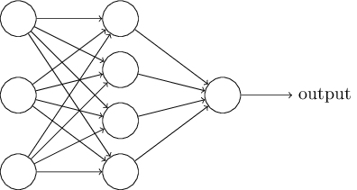
Introduction
Artificial intelligence, often abbreviated AI, is a branch of computer science concerning the intelligence of machines. More specifically, artificial intelligence is the ability of inorganic automaton to perceive their environment and make rational decisions based on data acquired. Used in applications with dynamic environments, as opposed to static, AI attempts to provide solutions to problems without the need of human interaction. The entire purpose behind utilizing AI is to allow automata to make decisions as if it were human. In essence, AI is an effort to emulate the human mind in settings where a real human would be impossible or impracticable to use.
Characteristics of AI
In the game industry, AI allows a CPU to compete against a human player (or another CPU) under the rules governing the game. For example, a chess AI will analyze the game and attempt to make moves which will maximize its success. Other examples of AI include speech recognition used in cell phones, automatic thermostat controls, and the navigation system used in autonomous robotic vacuum cleaners. In each of these applications, AI combines multiple elements together to complete a task based on the data presented. Breaking the AI into individual qualities allows these elements to be characterized.
In order for a system to be considered artificially intelligent, it must exhibit at least three established characteristics. These characteristics are referred to as the “three A’s”; acquire, analyze, action.
Acquire
An AI system has the ability to make observations about its environment.
Whether the observations are physical or purely numerical, they represent data acquired by the AI.
Analyze
An AI system has the ability to evaluate the data acquired and arrive at a conclusion. A chess AI will analyze board piece locations to determine a set of possible actions which will maximize its probability of winning the game.
Action
An AI system has the ability to make rational choices based on the conclusion of the analysis. This characteristic is especially important as it represents the AI’s function as an agent. In other words, the AI has the ability to choose its course of action, doing so in a rational manner.
The three A’s were specifically chosen in order to differentiate true AI from what is otherwise an automated entity performing a predetermined set of tasks. Industrial robots may appear to have AI; however, they are simply machines following programmed instructions. They do not have the ability to acquire nor analyze environmental data. Another misleading use of the word AI is toward game opponents. Often, game opponents that give the impression of being artificially intelligent are nothing more than controlled systems abiding by a set of rules according to the current situation. An example would include Goombas and Koopa Troopas commonly found throughout many Mario series. They do not have AI since they do not possess the defining characteristic of action. In other words, they do not have the ability to make choices. Although Goombas and industrial robots do not have AI, this doesn’t mean that they could not utilize AI.
For example, the industrial robot could be equipped with a humidistat and sound level meter in order to collect data about environmental humidity and decibel levels respectively. The robot could then analyze the information and make decisions based on the results of the analysis. A possible action may be to activate evaporation fans if the humidity rises above a certain level or to reduce operation speed if the environment decibel levels exceed regulation. While less independent, as may be associated with AI, the industrial robot in this proposed setting abides by the rules established for characterizing artificial intelligence. The robot has the ability to acquire, analyze, and take action based on environmental data, making rational decisions towards achieving a goal.
Understanding AI
Developing artificial intelligence involves critical thinking and requires an interrogative approach towards its application. It is often necessary to analyze human thought patterns when designing an AI. The process through which an individual arrives at a conclusion in a game of checkers is likely similar to the sequence of steps an AI should take to maximize competency. Thus to better understand artificial intelligence, it is worthwhile to consider the entity from which it is being modeled, the human brain.
With estimated 50-100 billon neurons and approximately 100 trillion synaptic connections linking the neurons, the human brain is arguably the most powerful computer in existence.
Prerequisites
Logic
In order to take action based on what it analyzes, an AI must use logical and conditional statements pertaining to the operation it has been programmed to do. For example, in a game of "Tic Tac Toe", the AI must be able to use logic statements to determine where to place the next 'X' or 'O' in order to either block its opponent or complete a 3-in-a-row for itself. Logic statements can also be used to put certain actions at a higher priority than others. For example, a "Tic Tac Toe" AI will attempt to complete its own 3-in-a-row before blocking the opponent, because if it has already won, then the game is over and there is no chance of the opponent winning.
Procedural Programming
Control Flow
Data Structures
Environment
Code Structure
Gather Variables
Components
Thinking like AI
To program an AI you must think like one. As a human, you can base your actions on your assessment of the situation — which move would be more strategic, which might result in a better outcome for you — while an AI cannot do this. It can only do what your code tells you to do, nothing more.
Conditionals
Conditionals are programming objects that check if an event is true and run a section of code if it is. In Ti Basic, the most applicable conditional for AI is If, and less common, While(, Repeat(,
For(, IS>(, and DS<(. Conditionals are the easiest way to reach an action from input information (it represents Analyze of the "three A's").
Probability
In a game that contains random elements as a mechanic, such as dice, cards, and spinners, a good AI must account for them in a logical manner. One way to implement this would be to do a weighted average of all the possible options, based on the likelihood of each outcome and a calculable value for how well the game is going.
Methods
There are many methods that an AI can use to calculate a move, each with their own strengths and weaknesses. These are some of the most popular.
MiniMax
MiniMaxing is a method of AI in which each possible move is plotted on a tree, the computer finds the most achievable end state, and takes moves to reach that state. Note that the end state does not have to be the best possible state; for example, a MiniMax "Tic Tac Toe" AI won't try to attempt 3 in a row assuming that its opponent won't try to stop it. Instead, a MiniMax AI assumes that its opponent will make the best possible moves, and then find moves that lead to the worst possible 'best' moves: in other words, the minimum maximum. MiniMaxing is suited for AI that should play perfectly, and thus might not be a good fit for a fun game opponent. This approach works best for smaller, shorter games like "Tic Tac Toe" where there aren't too many moves to plot, and the number of possible moves decreases over time. MiniMaxing in a game such as "Chess" is much more difficult, due to there being an increasing, large number of moves, so much so that such an endeavor is currently infeasible. MiniMaxing also doesn't work well for real-time games where each 'turn' happens every interactable frame.
Decision Tree
The decision tree AI is the most common and the most applicable AI in video games (and is also the easiest to implement on a graphing calculator). A decision tree's foundation is the conditional. The programmer codes in certain events, has the computer check if those events are true, and then has it run code if it is true. For the game "Tic Tac Toe", the programmer might have the computer check if it has a 2 in a row on the board. If so, then they will have it choose the 3rd empty tile. This approach to AI is the best suited for games due to its logical, predictable, and easy to implement system of conditionals. Because of the decision tree's simple nature, it is by far the best choice for TI Basic.
Self-Learning
First of all, letting a calculator learn is not really possible, though it is possible to let it remember and compare, thus creating the illusion of learning. Let's look at an example, "Tic Tac Toe": in this game it could be possible for the program to store all the games it's played in lists, whenever the program can't figure a good move using the normal routine it can refer back to the lists and compare the list with the actual situation, now if the situation matches it could give a good move based on what it did good or bad in the list it is comparing to. This way of learning would prevent the human player from applying the same tactic over and over again, ergo, the machine seems to have learned what to do when this "tactic" appears. A good example of self-learning is Deep Blue, an AI developed by IBM that won a deciding chess game against the best human chess player at the time.
[[embedvideo]]
[[/embedvideo]]
Conclusion
work in progress
ASCII Output Codes
The following table proposes an extension to the (incomplete) set of ASCII codes classically exported by TI-GRAPH LINK, emulated by those with limited access to better portrayals of targeted characters, and utilized by those seeking to preserve their content in the 7-bit range. Each consists of no more than eight characters.
Cells containing symbols that already have 7-bit encodings are omitted. This includes letters and digits, brackets and other punctuation, and the alternate figures found on the number keys of most keyboard layouts. Each of these items can be typed out like normal, or encased in backslashes wherever convenient or necessary.
This is an alternative, often last-resort approach to rendering the TI-83 Plus font on a computer. Environments that support UTF-8 might be more well-suited for Unicode characterizations that rise above the 7-bit limit. For ways to represent TI-83 Plus characters in their full splendor, see the TI-83 Plus Large Font article.
| || || || || ||~ Table of ASCII Output Codes |
| ||~ 01–7F | ||~ 80–A6 | ||~ A7–CD | ||~ CE–F4 |
|  01 | \n\ |
  80 | \0\ |
  A7 | \ograve\ |
  CE | ...\ |
|  02 | \u\ |
  81 | \1\ |
 ![]() A8 | \ocirc\ |
A8 | \ocirc\ |  CF | \<\ |
|  03 | \v\ |
  82 | \2\ |
  A9 | \ouml\ |
  D0 | \block\ |
|  04 | \w\ |
  83 | \3\ |
  AA | \Uacute\ |
  D1 | \per\ |
|  05 | >\ |
  84 | \4\ |
  AB | \Ugrave\ |
  D2 | -\ |
|  06 | \squp\ |
  85 | \5\ |
 ![]() AC | \Ucirc\ |
AC | \Ucirc\ |  D3 | \area\ |
|  07 | \sqdown\ |
  86 | \6\ |
  AD | \Uuml\ |
  D4 | \^box\ |
|  08 | \intgrl\ |
  87 | \7\ |
  AE | \uacute\ |
  D5 | \^3\ |
|  09 | \x\ |
  88 | \8\ |
  AF | \ugrave\ |
  D6 | \enter\ |
|  0A | \box\ |
  89 | \9\ |
 ![]() B0 | \ucirc\ |
B0 | \ucirc\ |  D7 | \i\ |
|  0B | \cross\ |
  8A | \Aacute\ |
  B1 | \uuml\ |
  D8 | \p^\ |
|  0C | \dot\ |
  8B | \Agrave\ |
  B2 | \Ccedil\ |
  D9 | \chi\ |
|  0D | \subT\ |
 ![]() 8C | \Acirc\ |
8C | \Acirc\ |  B3 | \ccedil\ |
  DA | \statF\ |
|  0E | \root3\ |
  8D | \Auml\ |
  B4 | \Ntilde\ |
  DB | \e\ |
|  0F | \hexF\ |
  8E | \aacute\ |
  B5 | \ntilde\ |
  DC | \L\ |
|  10 | \root\ |
  8F | \agrave\ |
  B6 | \acute\ |
  DD | \N\ |
|  11 | \^-1\ |
 ![]() 90 | \acirc\ | || ... |
90 | \acirc\ | || ... |  DE | ))\ |
|  12 | \^2\ |
  91 | \auml\ |
  B8 | ..\ |
  DF | \blk->\ |
|  13 | \/_\ |
  92 | \Eacute\ |
  B9 | \iquest\ |
  E0 | \cursor\ |
|  14 | \o\ |
  93 | \Egrave\ |
  BA | \iexcl\ |
  E1 | \2ndcur\ |
|  15 | \r\ |
 ![]() 94 | \Ecirc\ |
94 | \Ecirc\ |  BB | \alpha\ |
  E2 | \Acur\ |
|  16 | \^T\ |
  95 | \Euml\ |
  BC | \beta\ |
  E3 | \acur\ |
|  17 | \<=\ |
  96 | \eacute\ |
  BD | \gamma\ |
  E4 | \inscur\ |
|  18 | !=\ |
  97 | \egrave\ |
  BE | \Delta\ |
  E5 | \ins2nd\ |
|  19 | >=\ |
 ![]() 98 | \ecirc\ |
98 | \ecirc\ |  BF | \delta\ |
  E6 | \ins_A\ |
|  1A | (-)\ |
  99 | \euml\ |
  C0 | \epsil\ |
  E7 | \ins_a\ |
|  1B | \EE\ |
  9A | \Iacute\ | || ... |
  E8 | \gline1\ |
|  1C | ->\ |
  9B | \Igrave\ |
  C2 | \Lambda\ |
  E9 | \gline2\ |
|  1D | \10\ |
 ![]() 9C | \Icirc\ |
9C | \Icirc\ |  C3 | \mu\ |
  EA | \gabove\ |
|  1E | \uarrow\ |
  9D | \Iuml\ |
  C4 | \pi\ |
  EB | \gbelow\ |
|  1F | \darrow\ |
  9E | \iacute\ |
  C5 | \rho\ |
  EC | \gpath\ |
| || ... |  9F | \igrave\ |
  C6 | \Sigma\ |
  ED | \ganim\ |
|  24 | \^4\ |
 ![]() A0 | \icirc\ |
A0 | \icirc\ |  C7 | \sigma\ |
  EE | \gdot\ |
| || ... |  A1 | \iuml\ |
  C8 | \tau\ |
  EF | \upblk\ |
|  5B | \theta\ |
  A2 | \Oacute\ |
  C9 | \phi\ |
  F0 | \dnblk\ |
| || ... |  A3 | \Ograve\ |
  CA | \Omega\ |
  F1 | \chkrbd\ |
|  60 | \lsquo\ |
 ![]() A4 | \Ocirc\ |
A4 | \Ocirc\ |  CB | \xbar\ | || ... |
| || ... |  A5 | \Ouml\ |
  CC | \ybar\ |
  F3 | \squp_2\ |
|  7F | \=\ |
  A6 | \oacute\ |
  CD | \^x\ |
  F4 | \szlig\ |
Asm command

| Command Summary | Command Syntax | Calculator Compatibility | Token Size |
|---|---|---|---|
| Runs an assembly program. | Asm(prgmNAME) | TI-83+/84+/SE (not available on the regular TI-83) |
2 bytes |
Menu Location
This command is only found in the catalog. Press:
1. 2nd CATALOG to access the command catalog.
2. DOWN six times.
3. ENTER to select Asm(.
The Asm( Command
The Asm( command is used for running an assembly program. Unlike TI-Basic programs, assembly programs are written in the calculator's machine code directly, which makes them more powerful in both speed and functionality. However, it also means that if they crash, they crash hard — there is no built-in error menu to protect you.
Keep in mind that many assembly programs these days are written for a shell such as Ion or MirageOS. If you're dealing with one of those programs, calling Asm( on it will do nothing; you need to get the appropriate shell and run that instead.
With the AsmPrgm and AsmComp( commands, you can create small assembly programs yourself, directly on the calculator. If you are using at TI-84+CE with OS 5.3, the Asm( is unnecessary to run such programs.
Error Conditions
- ERR:INVALID is thrown if the program isn't an assembly program.
Related Commands
See Also
Asm (disambiguation)
The abbreviation "asm" is ambiguous and may refer to:
- Asm(, the command used for running a shell-independent assembly program.
- Assembly, the other programming language available on the TI graphing calculators.
If an internal link led you here, you may wish to change the link to point directly to the intended article.
Asm84CEPrgm
Please see the AsmPrgm page. The functionality and use are the same between both commands. However, the Asm84CEPrgm is only available on the TI-84+CE calculator. Keep in mind that hexadecimal for the monochrome calculators may not work on color calculators. This token does not work on OS 5.3.1, it has been deprecated by Texas Instruments for no good reason. Even uploading a program with this token in it will not work as it will throw an INVALID error.
There is a workaround to this problem. A sendable program containing the command can be found here.
To run assembly programs on the calculator, recall the command from the program you sent. Type your hex code in the editor. When you're done, quit the program. Type the following on the homescreen:
AsmComp(prgmNAME1,prgmNAME2
Then, find the program you compressed and run it with either the Asm( command or like a normal BASIC progam.
The Asm84CPrgm Command
Please see the AsmPrgm page. The functionality and use is the same between both commands. However, the Asm84CPrgm is only available on the TI-84+CSE calculator. Keep in mind that hexadecimal for the monochrome calculators may not work on color calculators.
Basic Builder
DIY Assembly Library
Assembly Hex Codes
Assembly Libraries
Assembly Shells
Asmcomp

| Command Summary | Command Syntax | Calculator Compatibility | Token Size |
|---|---|---|---|
| Compresses an assembly program in hexadecimal form into binary form. | Asm(prgmORIGINAL,prgmRESULT) | TI-83+/84+/SE/CSE/CE (not available on the regular TI-83) |
2 bytes |
Menu Location
This command is only found in the catalog. Press:
1. 2nd CATALOG to access the command catalog.
2. Scroll down to AsmComp( and press enter.
The AsmComp( Command
This command is used to compress an assembly program written using AsmPrgm into an "assembled" assembly program. This will make the program about twice as small, and protect it from being edited, in addition to making execution faster.
To use AsmComp(, give it the ASCII represented assembly program, followed by the name you want the assembled program to have. That name can't be already taken. Since it's not easy to rename an assembled assembly program, if you want to write a program called prgmGAME, you type the ASCII represented code in a program with a different name (e.g. GAMEA) and then do AsmComp((prgmGAMEA,prgmGAME).
Assembly programs can be run with Asm(.
Error Conditions
- ERR:DUPLICATE is thrown if prgmRESULT is an already used program name;
- ERR:INVALID is thrown if prgmORIGINAL doesn't start with
AsmPrgm; - ERR:SYNTAX is thrown if prgmORIGINAL is not an assembly program.
Related Commands
Assembly Libraries
Assembly libraries are commonly used by TI-Basic programs to provide features that enhance them. Since TI-Basic programs don't have access to any of the internal functions of the calculator and the peripherals, assembly libraries can bridge that gap. The only caution about using assembly programs is that you need to make sure to include the assembly program if you give your program to someone else.
- Auto Power-Down — This tool allows BASIC programmers to implement an APD feature into their main loop. An example is included. An 84+ is recommended (but not altogether necessary) to implement this into a BASIC program. Note: This program will work with OnBlock. Even if OnBlock is enabled, when using this program, the user will be able to turn the calculator back on and continue with the execution of the program.
- BASIC Tools — BASIC Tools is a really neat set of assembly programs which can be used to allow BASIC programs to have really neat featues. BASIC Tools allows BASIC programs to inverse text, power off the calculator mid-program, change the contrast level, shift the screen up, determine the current contrast level, enable alphalock, determine the amount of free RAM, and check the batteries!
- CELTIC — This is an ASM utility to be used with BASIC programs that will empower BASIC programs to perform a variety of functions that BASIC would not previously allow, including the ability to read or write appvars and programs and swap variables between RAM and Archive.
- Codex — This is an awesome asm utility for basic programmers. It includes 32 assembly functions that basic programmers can use. It is centered mostly upon graphical functions. Yet there are some other miscellaneous functions. I believe it is one of the most complete utilities for basic programmers.
- Custom pics — This program allows you to save an unlimited number of pics with custom names. The pictures are stored in lists of 786 bytes. program size:182 bytes. my first ASM program. No shell needed.
- Flash Gordon — It's the famous Flash Gordon, with two subroutines that I've written to make this great program less of a pain in a neck. Basically, what it does is that you run this, and you don't have archive/unarchive your programs: they all stay in the archive, which means faster loading and less wear and tear on the flash memory.
- Graph Screen Wipes — This is a collection of 8 screenwipes. They will take whatever is in the graph buffer and move it up, left, down, right, up+left, up+right, down+left or down+right. Useful as a subroutine in either basic or assembly programs. Same principle behind side-scrolling games... except this shows how to do diagonal as well as left, right, up and down. 2nd release: Bugfree as far as I know. Also contains a demo program to demonstrate what it does. 3rd release: Now supports user defined scrolling amounts (store a number in X, and the screen will be scrolled that many lines).
- GreyPic8x — This program takes three pics (pic1, pic2 & pic3) and converts them into a greyscale screen. Very useful for Basic programmers if they want a greyscale title picture.
- Instant Graph Inverse — This program takes the graph buffer and inverses it (very quickly). Very useful as a subroutine for either basic or assembly programs.
- InstCirc — InstCirc is an ASM program designed to be callable from within TI-BASIC programs. It allows BASIC users to create circles much faster than the built in TI-OS routine. This is NOT another 4-part circle drawing flag enabler that so many other fast circ programs are.
- Inverter — The impetus for this program came from all the low quality BASIC graphics programs I've seen posted at ticalc.org, most of which deal with inverting large portions of the screen. Well, in my humble opinion, that sort of thing is best handled in ASM instead. Thus, here is an exceedingly fast and small full screen inverter. It inverts the screen instantaneously and is only 36 bytes!
- Omnicalc — Omnicalc integrates additional functionality into your 83+'s operating system. For example, it adds more functions for BASIC programmers, base conversions, and compressed programs, among other things. This latest version provides bug fixes, including the ability to now transfer and group BASIC programs using Omnicalc functions.
- OnBlock — A simple program that installs an interrupt that blocks the use of the On Break in basic programs.
- Picture Manager — This program merges the capabilities of ZPIC, ZSTO and a few new functions into 1 program. Basically, you can archive/unarchive/delete/recall/store up to 255 different pictures on your calculator! It also returns various error codes in case something went wrong (like bad input), so the program wont error out! This is MOST useful in graphics-intensive programs, like BASIC picture editors and BASIC games.
- RAGE — It accepts lists now instead of several vars. Also, the best improvement is the new support of user defined sprites. Games like Tetris, Duckhunt, Chess, Checkers, and Monopoly are now easily possible in Basic. Check it out if you'd like an alternative to xLib or Omnicalc, as this takes up less than 1K and is fully customizable.
- Resource — This routine is very useful for everyone. You can save a lot of free RAM memory when using Resource. It copies programs (TI-Basic and Asm) to RAM from Archive; so they only need free RAM when they are running! The routine could be used within TI-Basic programs or stand-alone at home screen!
- Screen Shot Maker — This program lets you take a screen shot of the graph and saves it as an assembly program. The new program, when you run it, copies the picture to the graph and displays it. This is useful for Basic programmers that are writing graphics-heavy programs and have run out of pics. This version is bug-free. If you don't like the program much, it does have a nice string input routine you might like.
- Symbolic — This application installs new functions onto your calculator. These can be used anywhere in the TI-83+ OS. These functions include a symbolic differentiation and simplification. Great for a lot of math classes.
- TLIB — This library is written for BASIC programmers who want to use ASM's advantages without having do learn this difficult language ! With TLIB, you can : - Run the indicator OFF - Clear the screen with horizontal and vertical lines (it is not really faster than BASIC : 6sec instead of 8sec ) - Do a pause (with a countdown) - Switch off the calculator - Inverse all the pixels of the plot screen - write in video inverse mode - and cancel this "video inverse mode".
- Variable Status — This little package can identify if a variable/program/whatever exists and whether or not it is archived. It can also determine if a program is ASM or BASIC!
- XKeys — A library that allows BASIC to detect multiple key presses. I've also included a demo that shows how to detect the arrow keys. The readme explains in more detail and includes a key code chart. This was designed with games in mind so it is small, fast, and easy to use. This version does not use interrupts or any safe RAM areas, so it should be safe to use with other libraries.
- xLIB — An APP that adds functionality to TI-83/4+ BASIC programs. It installs a parser hook which will intercept any real( requests. See the xLIB article for more information about it.
- Xtravar Beta 1 — Xtravar Beta 1 is a no-shell assembly program that lets you use up to 256 different strings, matrices, pics, etc. It also lets you use special characters. The best part is that you can send your program to other calcs and they won't need this program to run it!
- ZBASIC Library — ZBASIC is a set of 10 ASM routines which BASIC programs can access and use. These include inverting the screen, getting free RAM amount, setting/checking contrast level, getting battery status, shifting the screen up, etc.
- ZBTools — Assembly Tools for Basic Programmers. It provides several useful functions for TI-Basic programmers.
- Celtic III — Celtic III is a Flash Application for the TI-83 Plus, TI-83 Plus Silver Edition, TI-84 Plus, and the TI 84 Plus Silver Edition graphing calculators [ TI-83/84+(SE), designed to extend the functionality of these calculators so that BASIC games and utilities can perform actions that cannot easily be done through the language itself. Celtic III includes all commands from Xlib and some from OmniCalc.
Asmprgm

| Command Summary | Command Syntax | Calculator Compatibility | Token Size |
|---|---|---|---|
| This command must be the beginning of an assembly program. | AsmPrgm | TI-83+/84+/SE/CSE/CE (not available on the regular TI-83) |
2 bytes |
Menu Location
This command is only found in the catalog. Press:
1. 2nd CATALOG to access the command catalog.
2. Scroll down to AsmPrgm and press ENTER.
The AsmPrgm Command
This command denotes the start of an assembly program in hexadecimal form. The command must go at the beginning of a program.
Using AsmPrgm is the only built-in way to create assembly programs on the calculator, and it's not very convenient. To use it, after AsmPrgm itself, you must type in the hexadecimal values (using the numbers 0-9, and the letters A-F) of every byte of the assembly program. Even for assembly programmers, this is a complicated process: unless you've memorized the hexadecimal value of every assembly command (which is about as easy as memorizing the hexadecimal value of every TI-Basic token) you have to look every command up in a table.
In addition, it's easy to make a typo while doing this. For this reason, it's recommended not to use AsmPrgm to write assembly programs on the calculator, but instead write assembly programs on the computer. This also lets you use emulators and debuggers and such, as opposed to crashing your calculator (possibly permanently) every time you have a bug.
Just about the only use for AsmPrgm is to enter the hex codes for simple assembly routines that can be called from Basic programs or used for some other short task. For example, the following program will allow you to type in lowercase letters (by pressing ALPHA twice, you go into lowercase letter mode):
AsmPrgmFDCB24DEC9
To use this, create a program, and enter the code above into it. Then run the program using Asm(. Voila! Lowercase letters are now enabled.
More such short programs can be found here.
TI-84+ Color Calculators
For the TI-84+ C series of calculators, AsmPrgm has been replaced by two new commands: AsmPrgm84C for the TI-84+ CSE and AsmPrgmCE for the TI-84+ CE. The commands function in the exact same manner as the original AsmPrgm command. However, it is important to note that sending assembly programs between a CSE and CE (or vice versa) may cause errors due to a difference in commands.
Many of the hex codes involving AsmPrgm also no longer function correctly on C series calculators. The updated hex codes can be found here. Please note, however, that directly entering hex codes has been disabled on the CE with OS 5.3.1; attempting to view AsmPrgmCE in the catalog will show the command crossed-out. Hex codes can be still be run from older programs.
Related Commands
See Also
Assembly Shells
Assembly shells are programs that can be loaded onto your calculator and act as an interface for running other programs. They also provide extra functionality like giving access to key-hooks. This page provides you with code you can embed into TI-Basic programs to make them compatible with assembly shells.
MirageOS
MirageOS is currently the most common assembly shell. To make a TI-Basic program appear in the MirageOS menu, put a colon (":") as the first line of the program:
::
:<program code...>
Optionally, you may include a description for the program:
::"<program description>
:<program code...>
As a warning, there have been cases of MirageOS not running TI-Basic programs correctly; after the program finishes, the calculator will crash.
Doors CS
Doors CS by Kerm Martian is the most recent assembly shell released. It offers the same functionality as MirageOS along with several other features, although it utilizes a mouse cursor and a different user interface. You can have Doors CS display a custom icon by adding one of the following to your programs:
::DCS
:"<16 character hex code for 8x8 icon>
or
::DCS6
:"<64 character hex code for 16x16 icon>
or
::"<program description>
::DCS
:"<16 character hex code for 8x8 icon>
or
::"<program description>
::DCS6
:"<64 character hex code for 16x16 icon>
You can also have Doors CS not display your program (for small subroutines that you don't want users playing with):
:Ans
:<program code>
Kerm Martian has also released a version of Doors CS that is compatible with the TI-84+CSE. This shell operates in much the same way and has the same arguments for creating icons and preventing the display of programs. Doors CSE comes with the Celtic and EXLIBC. This shell can be found at cemetech.net or ticalc.org
Doors CE is currently undergoing development. The last official update places Doors CE under the debugging stage. It will be similar to Doors CSE, but for the TI-84 CE. You can follow the development thread here.
Noshell
Noshell (pronounced 'nosh-ell') is a flash application for running any program that appears in the program menu like you would a TI-Basic program. It will automatically run all programs.
CrunchyOS
CrunchyOS is another common assembly shell. To make your TI-Basic program compatible with CrunchyOS, add a colon as its first line:
::
:<program code>
Other Shells
The other assembly shells, especially the older ones, don't have an option to run TI-Basic programs; you just have to use the program menu instead. Ion is probably the most notable shell that doesn't run TI-Basic programs.
Assembly Libraries
Assembly Shells
Assembly
Besides TI-BASIC, assembly is the other primary programming language available for the TI-83 series calculators. Unlike TI-BASIC, which uses commands and functions that are easy to understand, assembly is programmed in the calculator's own machine language. Thus, it is much harder to program in and read.
This lack of usability, however, is more than made up for when you consider the fact that assembly is much faster and more feature rich than TI-BASIC. Games that normally can't be done (or, if they can be done, they aren't done very well) in TI-BASIC are just considered average in assembly.
At the same time, there aren't as many assembly programmers compared to TI-BASIC programmers; and subsequently, effort has been made to enhance TI-BASIC using assembly, to make it more capable of quality games and programs. This includes:
- Shells — A shell allows a person to run a program from inside one central place, and since most assembly programs are run through a shell, it makes sense to run your TI-BASIC programs there as well.
- Libraries — A library enhances a TI-BASIC program in some way, providing support to an internal function of the calculator (such as lowercase text) or access to a peripheral of the calculator (such as the USB port on the TI-84+/SE). If the ones available do not suit you, you can even make your own.
- Applications — BASIC Builder allows you to package your TI-BASIC program(s) into a Flash application, which appears in the APPS menu and gets executed just like a regular assembly application.
The TI-BASIC language itself provides three commands — Asm(, AsmPrgm, and AsmComp( — for running and compiling shell-independent assembly programs, which you simply run from the home screen or inside a program. Writing these kinds of assembly programs is actually more difficult, however, because the assembly language instructions are represented as hexadecimal numbers. There are some short assembly programs that can be written on the calculator and be of great use to BASIC programmers.
Two additional commands for running assembly programs have been added on the TI-84 Plus and TI-84 Plus SE calculators: OpenLib( and ExecLib. They can be used for running routines from Flash application libraries that have been specifically written for use with these commands. So far, however, most major libraries use other methods, for compatibility with pre-TI-84 calculators. The only existing software that uses OpenLib( and ExecLib is usb8x, a library for advanced use of the TI-84 Plus/SE USB port. Here, compatibility is obviously out of the question.
(For more on assembly, visit z80 Heaven and WikiTI.)
The * Command
Augment

| Command Summary | Command Syntax | Calculator Compatibility | Token Size |
|---|---|---|---|
| Combines two lists or matrices into one. In the case of matrices, this is done horizontally rather than vertically. | augment(list1,list2 augment(matrix1,matrix2 |
TI-83/84/+/SE | 1 byte |
Menu Location
Press:
1. 2nd LIST to access the List menu
2. RIGHT to access the OPS submenu
3. 9 to select augment(, or use arrows
Alternatively, press:
1. MATRX (on the TI-83) or 2nd MATRX (TI-83+ or higher) to access the Matrix menu
2. RIGHT to access the MATH submenu
3. 7 to select augment(, or use arrows
The augment( Command
The augment( command is used to combine two lists or two matrices into one. For lists, this is done the obvious way: adding the elements of the second on to the elements of the first. For example:
augment({1,2,3,4},{5,6,7
{1 2 3 4 5 6 7}
The lists must have at least one value. If you attempt to augment(L₁,L₂) and either of the lists are empty, you will receive an error. If you're using this within a program, you may want to use dim() to check the size before performing an augment.
For matrices, the columns of the second matrix are added after the columns of the first matrix: an R by C matrix augmented with an R by D matrix will result in an R by (C+D) matrix. For example:
augment([[1][2]],[[3][4]
[[1 3]
[2 4]]
Combining 3 or more lists
The augment() command only accepts two parameters. If you need to combine 3 or more lists, you can nest the augment calls.
This will NOT work: augment(L₁,L₂,L₃)
But this will: augment(augment(L₁,L₂),L₃)
Just be sure that all lists have at least 1 value to prevent errors.
Advanced Uses
Use the T (transpose) command if you want to combine two matrices vertically, rather than horizontally. For example:
augment([[1,2]]T,[[3,4]]T)T
[[1 2]
[3 4]]
Optimization
You may be tempted to use augment( to add one element to the end of a list:
augment(L1,{X→L1
However, the following way is faster and more memory-efficient while the program is running (although it increases the program's size):
X→L1(1+dim(L1
Error Conditions
- ERR:DATA TYPE is thrown if you try to augment a single number to a list, a common error — use {X instead of X.
- ERR:DIM MISMATCH is thrown if you try to augment two matrices with a different number of rows.
- ERR:INVALID DIM is thrown if one of the arguments is a list with dimension 0, or if the result would have dimension over 999 (for lists) or 99x99 (for matrices).
Related Commands
Auto answer
| Command Summary | Command Syntax | Calculator Compatibility | Token Size |
|---|---|---|---|
| Mode command that sets Answers to AUTO. | AUTO Answer | TI-84 2.53MP only | 2 bytes |
Menu Location
Press:
1. MODE
2. DOWN until you see Answers
3. ENTER on AUTO
Alternatively, access the catalog.
The AUTO Answer Command
The AUTO Answer command is a mode command that changes the Answers mode to AUTO. The AUTO mode is in essence the same mode that lower OS models use. The calculator will evaluate a numerical expression and return a decimal or number in scientific notation, unless ►Frac is used.
In the Mathprint mode, no noticeable difference is seen unless the answer is converted to a fraction.
Related Commands
Avalanche
The basic premise behind Avalanche is to avoid the falling spikes ("V") by moving to the left or right, trying to see how long you can hold out for. It is somewhat more complex than Guess the Number, using nested loops, a list variable, and some fairly advanced optimizations. Try to understand the code, and actually put it in your calculator and try it out.
The Code
:ClrHome
:Disp "SPEED
:Disp "1) SLOW
:Disp "2) NORMAL
:Disp "3) FAST
:DelVar Z8→X
:Repeat 2>abs(Ans-2
:getKey-91→S
:End
:ClrHome
:Disp "SCORE:
:Repeat K=45 or max(X=L1
:Output(8,1," // 16 spaces
:2→F
:seq(3I-int(3rand),I,1,5→L1
:Repeat K=45 or F=8
:getKey→K
:min(15,max(2,X-(Ans=24)+(Ans=26→X
:Output(8,Ans-1," O // 1 space
:Output(F,1," // 16 spaces
:F+1→F
:For(I,1,5
:Output(Ans,L1(I),"V
:End
:Z+S→Z
:Output(1,7,Ans
:rand(4-S
:End
:End
:DelVar L1ClrHome
:Disp "YOUR SCORE:
:Pause Z
:ClrHome:"
The Download
In case you want to try the program on your calculator, you can download the program in .8xp format.
Axesoff

| Command Summary | Command Syntax | Calculator Compatibility | Token Size |
|---|---|---|---|
| Disables the X- and Y- axes on the graph screen. | AxesOff | TI-83/84/+/SE | 2 bytes |
Menu Location
Press:
1. 2nd FORMAT to access the format menu.
2. Use arrows and ENTER to select AxesOff.
The AxesOff Command
The AxesOff command disables the X and Y axes on the graph screen, so that they aren't drawn. They can be enabled again with the AxesOn command.
(the y=x line that is drawn when both Seq and Web modes are enabled is also controlled by this command)
Generally, the AxesOff command should be used at the beginning of the program to disable the axes if the program is going to use the graph screen, since the axes get in the way. However, you should consider using StoreGDB and RecallGDB to save this setting if that's the case.
Related Commands
Axeson

| Command Summary | Command Syntax | Calculator Compatibility | Token Size |
|---|---|---|---|
| Enables the X- and Y- axes on the graph screen. | AxesOn | TI-83/84/+/SE | 2 bytes |
Menu Location
Press:
1. 2nd FORMAT to access the format menu.
2. Use arrows and ENTER to select AxesOn.
The AxesOn Command
The AxesOn command enables the X and Y axes on the graph screen, so that they are drawn. They can be disabled with the AxesOff command.
(the y=x line that is drawn when both Seq and Web modes are enabled is also controlled by this command)
Related Commands
Backgroundoff

| Command Summary | Command Syntax | Calculator Compatibility | Token Size |
|---|---|---|---|
| Turns off the graph Background, setting it back to the default white color. | BackgroundOff | TI-84+CE/CSE | 2 bytes |
Menu Location
[2ND][PRGM][LEFT ARROW][2]
The BackgroundOff Command
The BackgroundOff command has only one purpose: turn the background off. Run the command on its own line in a program with no other characters or arguments.
:BackgroundOn BLUE //Makes background blue
:BackgroundOff //Makes background white again
Optimization
BackgroundOff does essentially the same thing as turning the background on to the color white, as shown below.
:BackgroundOn WHITE
can be
:BackgroundOff
Related Commands
Backgroundon

| Command Summary | Command Syntax | Calculator Compatibility | Token Size |
|---|---|---|---|
| Used to display a background image on the graphscreen | BackgroundOn Image# Background color Background # (0-24) |
TI-84+CSE and TI-84+CE | 2 bytes |
Menu Location
Press
1. 2ND DRAW to access the draw menu
2. Navigate to BACKGROUND submenu
3. Enter or 1 to select BackgroundOn
The BackgroundOn Command
With the introduction of color and a higher resolution screen than the monochrome calculators, the TI-84+CSE and TI-84+CE included the ability to display a background image on the graphscreen. The images variables are similar to the picture variables in that there 10 slots. In addition, functions can be drawn on top of images.
BackgroundOn recalls an image variable or color and displays it on the graphscreen.
:BackgroundOn Image1
is the same as
:BackgroundOn 1
Intrestingly, the following is a valid syntax, which fills the graphscreen with a light blue (18).
:15→B
:BackgroundOn B+3
In addition, BackgroundOn can be used to fill the graphscreen with a solid color. The color variables range from 10 to 24, blue to dark gray, as documented here. For example, BackgroundOn 12 will fill the graphscreen with black.
:BackgroundOn 12
Error Conditions
- ERR:DOMAIN is thrown if the number is not an integer between 0 and 24.
Related Commands
Backing Up Programs
| This article is currently in development. You can help TI-Basic Developer by expanding it. |
|---|
You just completed a project on your calculator you've been working on for quite a while. And you're wondering, "How can I back up my programs in case they get deleted?" This tutorial will teach you how to backup certain programs on your calculator or PC. Backing up is extremely important for keeping projects alive, and to not shoot yourself in the foot when you lose them all. Backing up on your calculator is one of the steps for backing up should you don't have a PC lying around. For starters,
let's talk about what specifically what types of files you can back up. You can back up anything; programs, lists, app vars, matrices, strings, all that stuff. But there's a price to pay when backing up. You must back up 2 or more files in your backup, else, it wont work. Another thing is you must have memory available. Backing up files must be in RAM, because the OS doesn't mess with files in archive. So without further ado, let's back up your projects!
Preparation
Ensure your files are in RAM, if they're in archive, un-archive them. Ensure you have archive space left, because back-ups are written to archive. On the calculator and across the Internet, back-ups are called groups. Groups are like "zip folders" containing files that were in RAM, and now in archive. These groups cannot be un-archived, so don't try to un-archive them.
Backing Up
To group your programs, press [2ND], [+], [⬆], then [ENTER]. Type in the name of the group of your back up. Press [ENTER] when you're finished. A menu will be shown indicating what files you can back up. If you are backing up many types of files (i.e., programs, pics, strings), it's best to select All-. All+ selects ALL files in RAM, so you want to do the second option to select specific files. Use the arrow keys to move the cursor up and down to scroll through all the files, and hit [ENTER]
to select the file you want. A little black square will indicate that file will be backed up. When you have selected all the files you want, hit [➡] and select the option "Done". Your calculator should say or so "Copying variables to group: group name", then after it will show "Done" when the back up is complete. You're done!
Warnings
Yes, there are some warnings that you need to know. When you backed-up your projects and there are some things you need to add/change, you do not need to constantly group your projects when you make small changes. Only do it once you make big changes. Doing so can slow the calculator down, and can sometimes do a back-up fail. Back-up fails is when the group fails to write to archive. Meaning, your calculator can simply shut off for no reason or just freeze at the "Grouping" screen. If it freezes, you are forced to remove a battery to escape this. RAM will be cleared the next time you turn your calculator on. Not although you lose your groups, you lose your projects as well. Why? Because they were in RAM when you attempted the back-up, and when it crashed, they remained in RAM when you removed the battery. So now, your projects are permanently gone.
Keeping those projects alive
To keep your stuff from being deleted, make two groups when you back up for the first time. Then, when you make big changes, you delete the first group, then back up your projects. After a while, when you make even more changes, delete and back up to the second group. Keep doing this back and forth until you are 100% done with your projects.
But... what if those groups get deleted? Then you have nothing to spare! So what do you do now when you have the groups in archive and don't want them both gone? Back them up to your PC.
Backing up to your computer
Back-ups on your PC are harder to lose compared to your calculator. Files from your calculator are stored to your computer's hard drive, so they're not lost when your PC crashes. Cool, huh? So what do you do to back up files to your PC? It's not that simple as you may think it is. You need a special software for your computer to communicate with your calculator. Connecting your calculator won't just show up in Connected Devices. Depending on your calculator model, you may need either software:
If you have a TI-84 Plus/SE/CSE/CE/T
Download TI-Connect CE. This software is made for the 84+ family, and has a easy-to-use user interface. Requires Admin privileges to install.
If you have a TI-83/+/SE, 89/Titanium, 85, 86, Voyage 200, etc.
Download TI-Connect. This software is made for any calculator, including the 84+ family. This software can get slow and annoying, but it's old. Expect it to be slow. Requires Admin privileges to install.
Now you have the software. But aren't you forgetting something? Oh yeah! A linking cable. This is another important necessity for backing up to your PC. Most TI models don't have Bluetooth or Wifi on it (Except the newer N-Spire calculators)! There are many different cables made specifically for your model/family. Links to purchase these will be added later, so stay tuned. Connect your calculator to your PC.
Backing up to your PC
Now make sure your calculator is on and has a good battery charge. Now find the software on your computer and open it. Find the option to send/upload files to your PC.
More detailed explanation will be explained later.
Wrapping Up
Now that you know how so send files to your PC and back up on your calculator, you can now not worry about losing anything!
gray|Changes will be made on-the-go, expect more content on this page.
Bal

| Command Summary | Command Syntax | Calculator Compatibility | Token Size |
|---|---|---|---|
| Calculates the remaining balance after n payments in an amortization schedule. | bal(n,[roundvalue] | TI-83/84/+/SE | 2 bytes |
Menu Location
On the TI-83, press:
1. 2nd FINANCE to access the finance menu.
2. 9 to select bal(, or use arrows and ENTER.
On the TI-83+ or higher, press:
1. APPS to access the applications menu.
2. 1 or ENTER to select Finance...
3. 9 to select bal(, or use arrows and ENTER.
The bal( Command
The bal( command calculates the remaining balance after n payments in an amortization schedule. It has only one required argument: n, the payment number. However, it also uses the values of the finance variables PV, PMT, and I% in its calculations.
The optional argument, roundvalue, is the number of digits to which the calculator will round all internal calculations. Since this rounding affects further steps, this isn't the same as using round( to round the result of bal( to the same number of digits.
Usually, you will know the values of N, PV, and I%, but not PMT. This means you'll have to use the finance solver to solve for PMT before calculating bal(); virtually always, FV will equal 0.
Sample Problem
Imagine that you have taken out a 30-year fixed-rate mortgage. The loan amount is $100000, and the annual interest rate (APR) is 8%. Payments will be made monthly. After 15 years, what amount is still left to pay?
We know the values of N, I%, and PV, though we still need to convert them to monthly values (since payments are made monthly). N is 30*12, and I% is 8/12. PV is just 100000.
Now, we use the finance solver to solve for PMT. Since you intend to pay out the entire loan, FV is 0. Using either the interactive TVM solver, or the tvm_Pmt command, we get a value of about -$733.76 for PMT.
We are ready to use bal(. We are interested in the payment made after 15 years; this is the 15*12=180th payment. bal(180) gives us the result $76781.55 — as you can see, most of the loan amount is still left to pay after 15 years.
Formulas
The calculator uses a recursive formula to calculate bal():
In the case that roundvalue is given as an argument, the rounding is done at each step of the recurrence (which virtually forces us to use this formula). Otherwise, if no rounding is done (and assuming I% is not 0), we can solve the recurrence relation to get:
Error Conditions
- ERR:DOMAIN is thrown if the payment number is negative or a decimal.
Related Commands
Bang Bang

| Program Summary | Program Size | Uses Libraries? | Calculator Compatibility | Author | Download |
|---|---|---|---|---|---|
| A quality version of the classic scorched earth game. | 3,670 bytes | No, it's pure TI-Basic | TI-83/84/+/SE | Sean Weeks | bangbang.zip |
Bang Bang is a scorched earth clone that involves two players methodically shooting missiles at each other until one of them blows up the other's base. There are three different missile sizes to choose from — small, medium, and large — and each of the missiles has advantages and disadvantages. In addition, there is a wind that affects the missiles, and thus changes which missile you use.
The main feature of this game is that it provides three different modes of gameplay: 1 player, playing against a target; 2 player, playing against another person; and vs. AI, playing against a challenging AI. In addition, the terrain is randomly generated, although you can specify your own custom terrain from the menu as well.
Basic Builder
Basic Graphing
Setting up your Graph screen
Using the window button you can acces the window menu. In this menu you can read the following:
- Xmin
- Xmax
- Xscl
- Ymin
- Ymax
- Yscl
- Xres
Xmin
This is the value on which the calculator starts the X-axis of the graph (the minimum value a X coordinate can have). For instance, you need the X-axis to go from -2 till 10. In that case you would enter -2 here
note: You must use the (-) button instead of the - button, the (-) button declares a negative value whilst the - button declares to subtract value A from value B.
Xmax
This is the value on which te calculator Ends the X-axis of the graph (the maximum value a X coordinate can have). For instance, you need the X-axis to go from -2 till 10. In that case you would enter 10 here.
Xscl
This is the value on which te calculator Draws a point along the X-axis of the graph. For instance, you need a point after each 5 values in that case you would enter 5 here
Ymin
This is the value on which the calculator starts the Y-axis of the graph (the minimum value a Y coordinate can have). For instance, you need the Y-axis to go from -2 till 10. In that case you would enter -2 here
note: You must use the (-) button instead of the - button, the (-) button declares a negative value whilst the - button declares to subtract value A from value B.
Ymax
This is the value on which te calculator Ends the Y-axis of the graph (the maximum value a Y coordinate can have). For instance, you need the Y-axis to go from -2 till 10. In that case you would enter 10 here
Yscl
This is the value on which te calculator Draws a point along the Y-axis of the graph. For instance, you need a point after each 5 values in that case you would enter 5 here
Xres
Needs to be edited
graphscreen
Basic greyscale
Basic Greyscale
Most people do not know that greyscale can be achieved outside of a extra ASM library like Xlib, greyscale is nothing more than a pixel flashing on and off so quickly that it apperas to be grey. The con of greyscale in Basic is that it can give ERR:MEMoRY when you are using a delay, furthermore, only one grey can be achieved. For instance this hardcoded"block"
Repeat 0
Pxl-Change(31,47
Pxl-Change(31,48
Pxl-Change(31,49
Pxl-Change(30,47
Pxl-Change(30,48
Pxl-Change(30,49
Pxl-Change(29,47
Pxl-Change(29,48
Pxl-Change(29,49
Pxl-Change(28,47
Pxl-Change(28,48
Pxl-Change(28,49
End
this very simple code will switch the pixels on and off rapidly, a delay could be added using a "for(" loop.
Basic Builder
There is a computer application for the purpose of turning a BASIC program(s) into a Flash application. It is known as Basic Builder (BB for short). There are several pros and cons, so in the end, it is just a personal choice, and dependent on how large the programs are.
Pros:
- Your programs are compressed, allowing more programs in an app than regular archived programs
- It will be run from the archive
- People can't edit it (sometimes is a con)
- Apps look more professional
Cons:
- If your program takes up very little space, it is a waste of archive to turn it into an app
- BB can only make single page applications (16384 bytes), so there is a limit to the size of your program(s). For games including programs that always remains in the archive memory and that are only copied into the RAM when needed (such as with Resource or xLIB app), you still need to keep these programs separate from the BasicBuilder app, which partially defeats its purpose.
- Picture files must be separate from the app if they are going to be used by Omnicalc, xLIB or Celtic III commands. Else, you will need to create installation code that is only ran the first time you run your program that will copy all pictures from BasicBuilder to the picture slots you want.
- You can't GOTO an error (sometimes good)
- You can't delete variables inside the app, although there is a workaround.
Using Basic Builder
TO-DO: Add some screenshots of the steps to go along with the word instructions.
These are step-by-step instructions on using Basic Builder.
Obtaining Basic Builder and Other Equipment
The most recent version of Basic Builder can be found here. You will need Wappsign to sign the app you create, which can be found with the 83+ Flash Debugger, which can be found here.
Installation
All you need to install is the Flash Debugger, so open that file and follow the installation instructions.
Building the Application Hex
The instructions for generating the hex are in the BB readme, steps 1~8, but I have the instructions below.
- Ensure that all needed files (programs, subprograms, and pictures) are available. It is easier if they are in the same directory
- Start up the BB executable
- There are four fields on the right. Change 'Application name' to the name of your app, and 'Outputfile' to '
.hex'. Leave the other two fields alone for now - Press the upper left button, the one with a sheet of paper and a green '+'
To understand the next few things, you have to understand what BB actually does. It creates an app, that when started, will normally just execute the main program. However, if you want the user to be able to execute multiple things from the beginning, you can create multiple menu items. These will be shown in the format of the Menu( command. An example of this is a pack with several games that you want the user to choose from. You have several menu options and the user is free to decide which one.
- After you pressed that button, you should have seen a field appear in the left. That is the menu entry for the horde of files you will now turn into some hex
- Change that field from program name to the text that you want shown for that menu option when BB is started
- Click 'Add program' on the right. Find your program. Do this over and over until you have all the necessary programs. Do the same for 'Add picture'
- If you want more menu options, click the paper-and-plus button in the upper-left and repeat
- Click 'Generate' in the lower-right
You should now have a .hex file in the BB directory.=, along with a small pop-up giving how much space was saved/how much space is left. But you can't do anything with this hex file... Yet.
Signing the Hexfile
- Click on Start -> All programs -> TI-83 Plus Flash Debugger -> Wappsign
- You should have a small program running, called Wappsign. There should be four check boxes on the right. Check the upper two and un-check the lower two.
- On the right of the 'Application' field, there should be a '...' button. Click it.
- Browse for your hexfile.
- Click 'Sign'.
Congratz! You should now have an application in the same directory as the hexfile!
Beginner Guide
Note: This page was originally created by AtionSong on the TI-Basic wiki, and has been added here because TI-Basic wiki is in the process of being merged with this wiki. In addition to this page, only those pages which weren't already duplicated on this wiki were added.
TI-BASIC is a rich programming language that can be used to create programs from the tediously simple to the outrageously complex. While playing these games is fun, one the most intellectually stimulating and rewarding things you can do is actually program these programs. If you own a TI-83 calculator or higher, you have everything you need to start programming your own TI-BASIC programs.
Guides
Basic Programming
Note: This page was originally created by AtionSong on the TI-Basic wiki, and has been added here because TI-Basic wiki is in the process of being merged with this wiki. In addition to this page, only those pages which weren't already duplicated on this wiki were added.
The Basics
Creating a New Program
To create a new program:
- Press the PRGM button on your calculator
- Scroll over to the "NEW" heading
- Press "ENTER"
- Enter the name for your program
- Press "ENTER"
Executing a Program
To execute a program:
- Press the PRGM button on your calculator
- Scroll down to the program you want to execute
- NOTE: If the program you want to execute has an asterisk () next to it, it is archived, and inaccessible.*
- Press "ENTER"
- Press "ENTER" again to begin the program
Editing a Program
To edit a program:
- Press the PRGM button on your calculator
- Scroll over to the "EDIT" heading
- Scroll down to the program you want to edit
- NOTE: If the program you want to execute has an asterisk () next to it, it is archived, and inaccessible.*
- Press "ENTER" to enter the edit screen
Beginning Programming
In order to see an actual example of what is being discussed, create a program (see above) and call it WIKI. Some parts of the tutorial will ask you to create programs to execute, and this is where you will write them. Also, there is not a description of where commands are found. To find a command, click on the link to it's page, where a complete location description can be found, as well as a more complete description of it's function.
ClrHome, Output(, and Pause
To begin your TI-BASIC education, let's begin with two of the simplest and most helpful commands, ClrHome (standing for Clear Home) and Output(.
ClrHome
On your calculator, press a bunch of numbers (more than 1 line). Now go to prgmWIKI and simply create one line of code: ClrHome. Execute the program.
You should be staring at a blank screen. This is precisely what ClrHome does: It gets rid of any text already on the home screen.
Output(
You may or may not have already noticed that on the calculator screen, all characters (numbers, letters, spaces, punctuation, etc.) take up the same amount of space. Your screen can hold 16 characters across and 8 characters down. When you execute an Output( command, you are telling your calculator at which of these spaces to write a certain piece of text. For example, create the following program:
Program:WIKI
:ClrHome
:Output(3,4,"TI-BASIC
If you execute it, you should see TI-BASIC printed on the third line at the fourth space.
Pause
Pause is one of the most unique TI-BASIC commands because it can only be used in one way: It will stop the program from executing any code that comes after it until the user presses "ENTER"
To show you how Pause works, create the following program:
Program:WIKI
:ClrHome
:Output(1,1,"PRESS PAUSE
:Pause
:Output(3,6,"THANK YOU
After the program printed PRESS PAUSE, you should have seen shifting dots in the up right corner of the screen, and the program did not continue to print THANK YOU until you pressed "ENTER".
Pause can also be used to display some text or a variable, such as in this next program.
Program:WIKI
:ClrHome
:Pause "PROGRAM PAUSED"
:5→X
:Pause X
Using ClrHome, Output(, and Pause Together
You have only learned how to execute three TI-BASIC commands thus far, but they are all you need to create many programs on graphing calculators. One of the most common ways is to create a textual cartoon or a joke. For example, you could create the following program:
Program:JOKE
:ClrHome
:Output(1,1,"HOW DOES A
:Output(2,1,"MATHEMATICIAN
:Output(3,1,"LOSE WEIGHT?
:Pause
:Output(5,1,"BINOMIALS!
:Pause
:Output(6,1,"(BUY NO MEALS)
See what programs you can create using ClrHome, Output(, and Pause!
Input, Analysis, and Direction
However, using only ClrHome, Output(, and Pause does not allow for a wide arrange of enjoyable games because it lacks three important factors: Input, Analysis, and Direction. To learn how to add these to your program, just Continue...
Different Paths
Note: This page was originally created by AtionSong on the TI-Basic wiki, and has been added here because TI-Basic wiki is in the process of being merged with this wiki. In addition to this page, only those pages which weren't already duplicated on this wiki were added.
Lbl and Menu
An important aspect of every program is allowing the user to feel like they have some control over what goes on in the program. There are a lot of ways to let users chose their own paths. But first, you need those paths to lead somewhere.
Lbl
Lbl (label) is a command that divides your program into different sections. While this is not very helpful on its own, you can add commands that direct the user to different labels.
Menu(
The Menu( function is used to create some pretty awesome looking menus in your programs. Better yet, it's really simple. Look on the Menu( page to see how easy it is to make a menu.
Using Lbl and Menu( Together
Let's make the following program:
Program:WIKI
:Lbl 1
:ClrHome
:Menu("I AM REALLY...","COOL",2,"SMART",3,"PRETTY",4
:Lbl 2
:Output(1,1,"YOU ARE COOL
:Pause
:Goto 1
:Lbl 3
:Output(1,1,"YOU ARE SMART
:Pause
:Goto 1
:Lbl 4
:Output(1,1,"YOU ARE PRETTY
:Pause
:Goto 1
This program lets the user feel as if they are in control. It lets them pick which of the given paths they want to take, and the choice they make affects what happens in the program. In the program, whichever word they choose will appear after YOU ARE on the screen. Using only Lbl, Menu(, Output(, Pause, and ClrHome commands, you have all the tools necessary to create a complete, nice looking Text Adventure. Click on the link to see a tutorial of how to create a text adventure.
If, Then, Else, and Goto
If
If is used as a normal conditional statement would, in conjunction with Then. This means that when you place it in a program with a condition next to it (like X=5 or N>P), the next line of commands will only be executed if the statement is true (unless a not( restriction is placed before it, in which case, it will only be executed if the statement is not true).
Then
When separated from an if command by a colon (e.x. If X:Then), will only perform the following line of text if the statement following the if statement is true.
Else
When you place an If/Then statement into a program, there are always two options: The If/Then statement is true or the If/Then statement is false. Placing multiple If/Then statements for the same condition can get confusing. Instead, you can place an Else command, which will only perform the text after it if the If/Then statement before it is false.
Goto
Goto will simply do one task: It will GoTo the indicated label (e.x. ''Goto 5'' will send the program to label 5).
Using If, Then, Else, and Goto Together
In order to get this program to work, we need to use one command you do not know yet: randInt(. All you need to know is that it will choose a random integer between the two indicated numbers and store it into the indicated variable. You will learn more about this command later.
Program:WIKI
:ClrHome
:randInt(1,10→X
:Output(1,1,X
:Pause
:If X>5:Then
:Goto 1
:Else
:Goto 2
:Lbl 1
:Output(2,1,"GREATER THAN 5
:Goto 3
:Lbl 2
:Output(2,1,"LESS THAN/EQUAL TO 5
:Goto 3
:Lbl 3
:Output(4,1,"END
This program will choose a random number between 1 and 10. It will then show you the number, and pause. If the value of the number is greater than 5, the program goes to label 1, and outputs GREATER THAN 5. If is is not, the program goes to label 1 and outputs LESS THAN/EQUAL TO 5 (the two spaces are put in to wrap the text to the next line). After, the program will go to label 3 and output END.
Note on Using If and Then
A common problem that new programmers run into is the difference between using "If/Then" commands as opposed to just "If" commands. Observe the two programs:
Program:IFTHEN
:ClrHome
:Input "NUM",X
:If X=5:Then
:Goto 1
:Else
:Goto 2
...
In this program, if the number is five, the program will go to label one. If not, it will go to label two. But what if you wanted to change the program so that it would go to a different label for each number one through five? You cannot use more than one If/Then command for a condition! You must follow an If/Then with an Else! Instead, use this program:
Program:IF
:ClrHome
:Input "NUM",X
:If X=1
:Goto 1
:If X=2
:Goto 2
:If X=3
:Goto 3
...
If the statement, does not meet any of the conditions, the program will just continue normally.
Input
Input
Input is one of the most important commands that could be put into a program. It will allow the user of the program to input data, then the data will get stored into a variable. For example, if '''Input "NUMBER:",X''' is put into a program, the program will print NUMBER:, then wait until the user enters data and presses enter. The data will be stored into the variable X. This can make programs, such as the one above, be much more enjoyable for the user. If we take the program above and substitute the randInt( command for an Input command, we get:
Program:WIKI
:ClrHome
:Input "NUMBER 1-10:",X
:Pause
:If X>5:Then
:Goto 1
:Else
:Goto 2
:Lbl 1
:Output(2,1,"GREATER THAN 5
:Goto 3
:Lbl 2
:Output(2,1,"LESS THAN/EQUAL TO 5
:Goto 3
:Lbl 3
:Output(4,1,"END
The part of the code that displayed X is no longer necessary, because the user will obviously know the number they chose. The program will then go through the same analysis, but with the inputted number instead of a random one.
Guessing Games
Using the Input command is the basis of nearly all programs that do not use Menu( or getKey (which you'll learn about later). One of the simplest programs you can make with it is a 1 or even 2 person Guessing Game. Check out the Guessing Game tutorial to see how to use the commands you know to create a game that you and your friends can enjoy.
Visual Magic
Note: This page was originally created by AtionSong on the TI-Basic wiki, and has been added here because TI-Basic wiki is in the process of being merged with this wiki. In addition to this page, only those pages which weren't already duplicated on this wiki were added.
Using the Graph Screen
In this section of the tutorial, you will learn how to use the Graph Screen to create visual programs.
A good way to start is to put INPUT into the program code alone. A line with simply Input will take you to the graphing screen and give you a cursor to click in the screen. You might want to take off the Axis, Grid, and Coordinates first, by putting AxesOff, GridOff, and CoordOff before the Input
TI-BASIC gives several functions for drawing to the graph screen which are easily accessible through the draw menu ([2nd][prgm]). For most programs that use the graph screen, it is a good idea to put "StoreGDB 1" at the beginning and "RecallGDB 1" at the end. This stores the current graph state and restores it at the end, so when you change the graph state by using a function like AxesOff, the graph screen doesn't stay changed after the program is finished.
The Text Function
Let's get started with a small hello world program graph screen style (I know, I hate hello world programs too, but bear with me). This program uses the Text( command and should display in a small font. All commands used are accessed from the draw menu and everything following a "//" is a comment and shouldn't be typed in.
Program:HELLO // Program name
:ClrDraw // Clear the graph screen
:Text(1,1,"Hello // Display text "Hello" at the top left corner of the screen
If you run it, you should see the word hello appear in the top left corner of the screen. Notice how we did not put "StoreGDB 1" at the beginning? It was not needed, because we did not change The screens axes or change the way the graph screen is shown. The text function draws on a different coordinate system. The X axis stays the same, but the y axis is up side down. This chart might help explain better
X-Axis
|_|1|2|3|4|5|6|7|8|9|
|1|_|_|_|_|_|_|_|_|_|
|2|_|_|_|_|_|_|_|_|_|
|3|_|_|_|_|_|_|_|_|_|
|4|_|_|_|_|_|_|_|_|_|
|5|_|_|_|_|_|_|_|_|_|
|6|_|_|_|_|_|_|_|_|_|
|7|_|_|_|_|_|_|_|_|_|
|8|_|_|_|_|_|_|_|_|_|
|9|_|_|_|_|_|_|_|_|_|
The Text function takes 3 arguments in the form of Text(x,y,text. They are used as follows
| Arg | Usage |
|---|---|
| x | The X coordinate of the text |
| y | The Y coordinate of the text |
| text | The text to be displayed |
Simple Graph Screen Text Animations
Note: The following is a very simple, very slow animation, but don't think this is all! There are many other ways to create text animations, many of which you will learn in this tutorial.
With the simple knowledge of the Text and ClrDraw functions, and knowing how to use a few basic loops, you can make your very own(very simple) text animation! Start your loop. We'll use a For( loop because they are considerably faster than all other loops, but any loop will do:
:For(C,1,50,2
Next, draw the text you want to draw to the screen:
:Text(C,1," (Your Text Here)
Add a time waster, so the loop doesn't go to fast for you to see:
:For(D,1,100
:End
Clear the Screen:
:ClrDraw
Close the first For loop:
:End
And we're done! That wasn't so hard, was it? No. Stick around, there are plenty more graph screen functions to learn about!
To be continued...
Better Code Timings
Instructions
First, write the name and model of your calculator in the table below, then use this code with an empty line in the "test code here" space to measure your loop overhead.
Add the number of iterations you used to the "iterations" column, and [time taken]/[iterations] to the "average" column. Then subtract your loop overhead from the result and list it in the "time" column.
FnOff
PlotsOff
0→Xmin
94→Xmax
-62→Ymin
0→Ymax
DispGraph //if it is a graphing command
startTmr→θ
Repeat checkTmr(θ
End
For(𝑛,1,[iterations]) //sequence variable 𝑛; note the closing parenthesis.
//test code here
End
checkTmr(θ+1
Math Commands
Home Screen Commands
| Command | Iterations | Average (ms) | Loop overhead (ms) | Time (ms) | Username |
|---|---|---|---|---|---|
| ClrHome | 1000 | 29 | 1.2 | 28 | kgmstwo |
| Disp " | 1000 | 51 | 1.2 | 50 | kgmstwo |
| Output(1,1," | 10000 | 3.8 | 1.2 | 2.6 | kgmstwo |
| Output(1,1,"A | 10000 | 4.4 | 1.2 | 3.2 | kgmstwo |
| Output(1,1,"AB | 10000 | 5.0 | 1.2 | 3.8 | kgmstwo |
| Output(1,1,"ABC | 10000 | 5.6 | 1.2 | 4.4 | kgmstwo |
| ClrHome | 1000 | 27 | .68 | 26 | kgmstwo |
Graphics Commands
| Command | Iterations | Average (ms) | Loop overhead (ms) | Time (ms) | Username |
|---|---|---|---|---|---|
| Pxl-On(0,0 | 10000 | 2.9 | 1.2 | 1.7 | kgmstwo |
| Pxl-Off(0,0 | 10000 | 2.9 | 1.2 | 1.7 | kgmstwo |
| Pxl-Change(0,0 | 10000 | 2.9 | 1.2 | 1.7 | kgmstwo |
| Horizontal -5 | 1000 | 36 | 1.2 | 35 | kgmstwo |
| Horizontal -5 | 1000 | 35 | .68 | 34 | kgmstwo |
| Vertical 5 | 1000 | 25 | 1.2 | 24 | kgmstwo |
| ClrDraw | 1000 | 101 | 1.2 | 100 | kgmstwo |
| StoPic Pic1 | 10000 | 4.7 | 1.2 | 3.5 | kgmstwo |
| StoPic Pic1 | 10000 | 4.2 | .68 | 3.5 | kgmstwo |
| RclPic Pic1 | 1000 | 28 | 1.2 | 27 | kgmstwo |
| Pt-On(10,-10 | 10000 | 4.1 | 1.2 | 2.9 | kgmstwo |
| Pt-On(10,-10 | 10000 | 4.5 | 1.2 | 3.3 | kgmstwo |
| Pt-On(10,-10 | 10000 | 4.0 | .68 | 3.3 | kgmstwo |
| :ZStandard:84→Xmin:72→Ymax:ZInteger | 100 | 220 | .68 | 220 | kgmstwo |
| 0->Xmin:1->DeltaX:0->Ymin:1->DeltaY | 1000 | 14 | .68 | 13 | kgmstwo |
| 0->Xmin:94->Xmax:-63->Ymin:0->Ymax | 1000 | 18 | .68 | 17 | kgmstwo |
| Line(5,0,5,-62 | 1000 | 27 | .68 | 26 | kgmstwo |
| Line(5,0,5,-62,0 | 1000 | 27 | .68 | 26 | kgmstwo |
| Line(0,-5,94,-5 | 1000 | 37 | .68 | 36 | kgmstwo |
| Line(0,-5,94,-5,0 | 1000 | 37 | .68 | 36 | kgmstwo |
| Line(10,-10,10,-10 | 10000 | 7.2 | .68 | 6.5 | kgmstwo |
| Line(10,-10,10,-10,0 | 10000 | 7.4 | .68 | 6.7 | kgmstwo |
note: multiple commands always on their own line.
Loop Overheads
| Command | Average (ms) | Username |
|---|---|---|
| For(n,1,100000) | .83 | kgmstwo |
| For(n,1,100000 | .69 | kgmstwo |
Calculators Used
| Username | Model | OS version |
|---|---|---|
| kgmstwo | 84+SE | 2.43 |
| lirtosiast | 84+ | 2.55MP |
Binary, Hexadecimal and Octal number system
Binary, hexadecimal, and octal refer to different number systems. The one that we typically use is called decimal. These number systems refer to the number of symbols used to represent numbers. In the decimal system, we use ten different symbols: 0, 1, 2, 3, 4, 5, 6, 7, 8, and 9. With these ten symbols, we can represent any quantity. For example, if we see a 2, then we know that there is two of something. For example, this sentence has 2 periods on the end..
When we run out of symbols, we go to the next digit placement. To represent one higher than 9, we use 10 meaning one unit of ten and zero units of one. This may seem elementary, but it is crucial to understand our default number system if you want to understand other number systems.
For example, when we consider a binary system which only uses two symbols, 0 and 1, when we run out of symbols, we need to go to the next digit placement. So, we would count in binary 0, 1, 10, 11, 100, 101, and so on.
This article will discuss the binary, hexadecimal, and octal number systems in more detail and explain their uses.
How a Number System Works
Number systems are used to describe the quantity of something or represent certain information. Because of this, I can say that the word "calculator" contains ten letters. Our number system, the decimal system, uses ten symbols. Therefore, decimal is said to be Base Ten. By describing systems with bases, we can gain an understanding of how that particular system works.
When we count in Base Ten, we count starting with zero and going up to nine in order.
0, 1, 2, 3, 4, 5, 6, 7, 8, 9, ...
Once we reach the last symbol, we create a new placement in front of the first and count that up.
8, 9, 10, 11, 12, ... , 19, 20, ...
This continues when we run out of symbols for that placement. So, after 99, we go to 100.
The placement of a symbol indicates how much it is worth. Each additional placement is an additional power of 10. Consider the number of 2853. We know this number is quite large, for example, if it pertains to the number of apples in a basket. That's a lot of apples. How do we know it is large? We look at the number of digits.
Each additional placement is an additional power of 10, as stated above. Consider this chart.
| 103| 102| 101| 100|
| --- | --- | --- | --- |
|digit|digit|digit|digit|
| 1000| 100| 10| 1|
| --- | --- | --- | --- |
Each additional digit represents a higher and higher quantity. This is applicable for Base 10 as well as to other bases. Knowing this will help you understand the other bases better.
Binary
Binary is another way of saying Base Two. So, in a binary number system, there are only two symbols used to represent numbers: 0 and 1. When we count up from zero in binary, we run out of symbols much more frequently.
0, 1, ...
From here, there are no more symbols. We do not go to 2 because in binary, a 2 doesn't exist. Instead, we use 10. In a binary system, 10 is equal to 2 in decimal.
We can count further.
| Binary | 0 | 1 | 10 | 11 | 100 | 101 | 110 | 111 | 1000 | 1001 | 1010 |
|---|---|---|---|---|---|---|---|---|---|---|---|
| Decimal | 0 | 1 | 2 | 3 | 4 | 5 | 6 | 7 | 8 | 9 | 10 |
| --- | --- | --- | --- | --- | --- | --- | --- | --- | --- | --- | --- |
Just like in decimal, we know that the more digits there are, the larger the number. However, in binary, we use powers of two. In the binary number 1001101, we can create a chart to find out what this really means.
| 26| 25| 24| 23| 22| 21| 20|
| --- | --- | --- | --- | --- | --- | --- |
| 1| 0| 0| 1| 1| 0| 1|
| || || || || 64+0+0+8+4+0+1|
| || || || ||~ 77|
Since this is base two, however, the numbers don't get quite as large as it does in decimal. Even still, a binary number with 10 digits would be larger than 1000 in decimal.
The binary system is useful in computer science and electrical engineering. Transistors operate from the binary system, and transistors are found in practically all electronic devices. A 0 means no current, and a 1 means to allow current. With various transistors turning on and off, signals and electricity is sent to do various things such as making a call or putting these letters on the screen.
Computers and electronics work with bytes or eight digit binary numbers. Each byte has encoded information that a computer is able to understand. Many bytes are stringed together to form digital data that can be stored for use later.
Octal
Octal is another number system with less symbols to use than our conventional number system. Octal is fancy for Base Eight meaning eight symbols are used to represent all the quantities. They are 0, 1, 2, 3, 4, 5, 6, and 7. When we count up one from the 7, we need a new placement to represent what we call 8 since an 8 doesn't exist in Octal. So, after 7 is 10.
| Octal | 0 | 1 | 2 | 3 | 4 | 5 | 6 | 7 | 10 | 11 | 12... | 17 | 20... | 30... | 77 | 100 |
|---|---|---|---|---|---|---|---|---|---|---|---|---|---|---|---|---|
| Decimal | 0 | 1 | 2 | 3 | 4 | 5 | 6 | 7 | 8 | 9 | 10... | 15 | 16... | 24... | 63 | 64 |
| --- | --- | --- | --- | --- | --- | --- | --- | --- | --- | --- | --- | --- | --- | --- | --- | --- |
Just like how we used powers of ten in decimal and powers of two in binary, to determine the value of a number we will use powers of 8 since this is Base Eight. Consider the number 3623 in base eight.
| 83 | 82 | 81 | 80 |
|---|---|---|---|
| 3 | 6 | 2 | 3 |
Each additional placement to the left has more value than it did in binary. The third digit from the right in binary only represented 23-1, which is 4. In octal, that is 83-1 which is 64.
Hexadecimal
The hexadecimal system is Base Sixteen. As its base implies, this number system uses sixteen symbols to represent numbers. Unlike binary and octal, hexadecimal has six additional symbols that it uses beyond the conventional ones found in decimal. But what comes after 9? 10 is not a single digit but two... Fortunately, the convention is that once additional symbols are needed beyond the normal ten, letters are to be used. So, in hexadecimal, the total list of symbols to use is 0, 1, 2, 3, 4, 5, 6, 7, 8, 9, A, B, C, D, E, and F. In a digital display, the numbers B and D are lowercase.
When counting in hexadecimal, you count 0, 1, 2, and so on. However, when you reach 9, you go directly to A. Then, you count B, C, D, E, and F. But what is next? We are out of symbols! When we run out of symbols, we create a new digit placement and move on. So after F is 10. You count further until you reach 19. After 19, the next number is 1A. This goes on forever.
| Hexadecimal | 9 | A | B | C | D | E | F | 10 | 11... | 19 | 1A | 1B | 1C... | 9F | A0 |
|---|---|---|---|---|---|---|---|---|---|---|---|---|---|---|---|
| Decimal | 9 | 10 | 11 | 12 | 13 | 14 | 15 | 16 | 17 | 25 | 26 | 27 | 28 | 159 | 160 |
| --- | --- | --- | --- | --- | --- | --- | --- | --- | --- | --- | --- | --- | --- | --- | --- |
Digits are explained as powers of 16. Consider the hexadecimal number 2DB7.
| 163 | 162 | 161 | 160 |
|---|---|---|---|
| 2 | D | B | 7 |
As you can see, placements in hexadecimal are worth a whole lot more than in any of the other three number systems.
Conversion
It is important to know that 364 in octal is not equal to the normal 364. This is just like how a 10 in binary is certainly not 10 in decimal. 10 in binary (this will be written as 102 from now on) is equal to 2. 108 is equal to 8. How on earth do we know this? What is 20C.38F16, and how do we find out?
Here is why it is important to understand how the number systems work. By using our powers of the base number, it becomes possible to turn any number to decimal and from decimal to any number.
Base to Decimal
So, we know that 3648 is not equal to the decimal 364. Then what is it? There is a simple method in converting from any base to the decimal base ten. If you remember how we dissected the numbers above, we used powers, such as 24, and ended up with a number we understand. This is exactly what we do to convert from a base to decimal. We find out the true value of each digit according to their placement and add them together.
In a formula, this algorithm looks like:
$$ V_{10} = v_pB^p+v_{p-1}B^{p-1}+...+v_1B+v_0 $$
Where V10 is the decimal value, v is the digit in a placement, p is the placement from the right of the number assuming the rightmost placement is 0, and B is the starting base. Do not be daunted by the formula! We are going to go through this one step at a time.
So, let us say we had the simple hexadecimal number 2B. We want to know what this number is in decimal so that we can understand it better. How do we do this?
Let us use the formula above. Define every variable first. We want to find V10, so that is unknown. The number 2B16 has two positions since it has two digits. p therefore is one less than that[^1], so p is 1. The number is in base 16, so B is 16. Finally, we want to know what v is, but there are multiple v's. You have v1 and v0. This refers to the value of the digit in the subscripted position. v1 refers to the digit in position one (the second digit from the right). So, v1 is 2. v0 is the first digit which is B. In the case of the conversion, you must convert all the letters to what they are in decimal. B is 11 in decimal, so v0 is 11.
Now, plug all this into the formula:
Therefore, 2B16 is equal to 43.
Now, let me explain how this works. Remember how digit placement affects the actual value? For example, in the decimal number 123, the "1" represents 100 which is 1102. The "2" is 20, or 2101. Likewise, in the number 2B16, the "2" is 2161, and the B is 11160.
We can determine the value of numbers in this way. For the number 3648, we will make a chart that exposes the decimal value of each individual digit. Then, we can add them up so that we have the whole. The number has three digits, so starting from the right, we have position 0, position 1, and position 2. Since this is base eight, we will use powers of 8.
| 82 | 81 | 80 |
|---|---|---|
| 3 | 6 | 4 |
Now, 82 is 64. 81 is 8. 80 is 1. Now what?
Remember what we did with the decimal number 123? We took the value of the digit times the respective power. So, considering this further...
| 364| 68| 4*1|
| 192| 48| 4|
Now, we add the values together to get 244. Therefore, 3648 is equal to 24410.
In the same way that for 123, we say there is one group of 100, two groups of 10, and three groups of 1, for octal and the number 364, there are three groups of 64, six groups of 8, and four groups of 1.
Decimal to Base
Just like how we can convert from any base to decimal, it is possible to convert decimal to any base. Let us say that we want to represent the number 23610 in binary, octal, and hexadecimal. What we need to do is pretty much reverse whatever we did above. There isn't really a good formula for this, but there is an algorithm that you can follow which will help accomplish what we want.
This algorithm may look confusing at first, but let us go through an example to see how it can be used. We want to represent 236 in binary, octal, and hexadecimal. So, let's try getting it to binary first.
The first step is to make p equal to \(\operatorname{int}(\sqrt[B]{V})\). B is the base we want to convert to which is 2. The V is the number we want to convert, 236. Essentially, we are taking the square root of 236 and disregarding the decimal part. Doing this makes p become 7.
Step two says to let v equal our number V divided by Bp. Bp is 27, or 128, and the integer part of 236 divided by 128 is 1. Therefore, our first digit on the left is 1. Now, we actually change V to become V minus the digit times the Bp. So, V will now be 236-128, or 108.
We simply repeat the process until the p becomes a zero. When p becomes zero, we complete the steps a last time and then end.
So, since V is now 108, p becomes 6. 108 divided by 26 is 1. The 1 goes to the right of the 1, so now we have 11. V becomes 44 since 108-64 is 44.
How?
Now you might be asking yourself how to read these numbers. Well, that’s not so difficult. First, I’ll give a general mathematical explanation which can be fit into one formula:
In human language: the value of the cipher in the number is equal to the value of the cipher on its own multiplied by the base of the number system to the power of the position of the cipher from left to right in the number, starting at 0. Read that a few times and try to understand it.
Thus, the value of a digit in binary doubles every time we move to the left. (see table below)
From this follows that every hexadecimal cipher can be split up into 4 binary digits. In computer language: a nibble. Now take a look at the following table:
| || || ||~ Binary Numbers| || |
| 8| 4| 2| 1| | Hexadecimal Value| Decimal Value|
| --- | --- | --- | --- | --- | --- | --- |
|0|0|0|0| |0|0|
|0|0|0|1| |1|1|
|0|0|1|0| |2|2|
|0|0|1|1| |3|3|
|0|1|0|0| |4|4|
|0|1|0|1| |5|5|
|0|1|1|0| |6|6|
|0|1|1|1| |7|7|
|1|0|0|0| |8|8|
|1|0|0|1| |9|9|
|1|0|1|0| |A|10|
|1|0|1|1| |B|11|
|1|1|0|0| |C|12|
|1|1|0|1| |D|13|
|1|1|1|0| |E|14|
|1|1|1|1| |F|15|
Another interesting point: look at the value in the column top. Then look at the values. You see what I mean? Yeah, you’re right! The bits switch on and off following their value. The value of the first digit (starting from the right), goes like this: 0,1,0,1,0,1,0,1,0,1,… Second digit: 0,0,1,1,0,0,1,1,0,0,1,1,0,0… Third digit (value=4): 0,0,0,0,1,1,1,1,0,0,0,0,1,1,1,1,… And so on…
Now, what about greater numbers? Therefore we’ll need an extra digit. (but I think you figured that out by yourself). For the values starting from 16, our table looks like this:
| || || || |~ Binary Numbers| || |
| 16| 8| 4| 2| 1| | Hexadecimal Value| Decimal Value|
| --- | --- | --- | --- | --- | --- | --- | --- |
|1|0|0|0|0| |10|16|
|1|0|0|0|1| |11|17|
|1|0|0|1|0| |12|18|
|1|0|0|1|1| |13|19|
|1|0|1|0|0| |14|20|
|1|0|1|0|1| |15|21|
|1|0|1|1|0| |16|22|
|1|0|1|1|1| |17|23|
|1|1|0|0|0| |18|24|
|1|1|0|0|1| |19|25|
|1|1|0|1|0| |1A|26|
|1|1|0|1|1| |1B|27|
|1|1|1|0|0| |1C|28|
|1|1|1|0|1| |1D|29|
|1|1|1|1|0| |1E|30|
|1|1|1|1|1| |1F|31|
For octals, this is similar, the only difference is that we need only 3 digits to express the values 1->7. Our table looks like this:
| || ||~ Binary Numbers| || |
| 4| 2| 1| | Octal Value| Decimal Value|
| --- | --- | --- | --- | --- | --- |
|0|0|0| |0|0|
|0|0|1| |1|1|
|0|1|0| |2|2|
|0|1|1| |3|3|
|1|0|0| |4|4|
|1|0|1| |5|5|
|1|1|0| |6|6|
|1|1|1| |7|7|
Conversion.
In the latter topic I explained the logic behind the binary, hexadecimal and octal number systems. Now I’ll explain something more practical. If you fully understood the previous thing you can skip this topic.
From decimal to binary
- Step 1: Check if your number is odd or even.
- Step 2: If it's even, write 0 (proceeding backwards, adding binary digits to the left of the result).
- Step 3: Otherwise, if it's odd, write 1 (in the same way).
- Step 4: Divide your number by 2 (dropping any fraction) and go back to step 1. Repeat until your original number is 0.
An example:
Convert 68 to binary:
- 68 is even, so we write 0.
- Dividing 68 by 2, we get 34.
- 34 is also even, so we write 0 (result so far - 00)
- Dividing 34 by 2, we get 17.
- 17 is odd, so we write 1 (result so far - 100 - remember to add it on the left)
- Dividing 17 by 2, we get 8.5, or just 8.
- 8 is even, so we write 0 (result so far - 0100)
- Dividing 8 by 2, we get 4.
- 4 is even, so we write 0 (result so far - 00100)
- Dividing 4 by 2, we get 2.
- 2 is even, so we write 0 (result so far - 000100)
- Dividing 2 by 2, we get 1.
- 1 is odd, so we write 1 (result so far - 1000100)
- Dividing by 2, we get 0.5 or just 0, so we're done.
- Final result: 1000100
From binary to decimal
- Write the values in a table as shown before. (or do so mentally)
- Add the value in the column header to your number, if the digit is turned on (1).
- Skip it if the value in the column header is turned off (0).
- Move on to the next digit until you’ve done them all.
An example:
Convert 101100 to decimal:
- Highest digit value: 32. Current number: 32
- Skip the "16" digit, its value is 0. Current number: 32
- Add 8. Current number: 40
- Add 4. Current number: 44
- Skip the "2" and "1" digits, because their value is 0.
- Final answer: 44
From decimal to hexadecimal.
THIS IS ONLY ONE OF THE MANY WAYS!
- Convert your decimal number to binary
- Split up in nibbles of 4, starting at the end
- Look at the first table on this page and write the right number in place of the nibble
(you can add zeroes at the beginning if the number of bits is not divisible by 4, because, just as in decimal, these don’t matter)
An example:
Convert 39 to hexadecimal:
- First, we convert to binary (see above). Result: 100111
- Next, we split it up into nibbles: 0010/0111 (Note: I added two zeroes to clarify the fact that these are nibbles)
- After that, we convert the nibbles separately.
- Final result: 27
From hexadecimal to decimal
*Check the formula in the first paragraph and use it on the ciphers in your hexadecimal number. (this actually works for any conversion to decimal notation)
An example:
Convert 1AB to decimal:
- Value of B = 160×11. This gives 11, obviously
- Value of A = 161×10. This gives 160. Our current result is 171.
- Value of 1 = 162×1. This gives 256.
- Final result: 427
From decimal to octal
- Convert to binary.
- Split up in parts of 3 digits, starting on the right.
- Convert each part to an octal value from 0 to 7
Example: Convert 25 to octal - First, we convert to binary. Result: 11001
- Next, we split up: 011/001
- Conversion to octal: 31
From octal to decimal
Again, apply the formula from above
Example: convert 42 to decimal
- Value of 2=80×2=2
- Value of 4=81×4=32
- Result: 34
Fun Facts
OK, these may not be 100% "fun", but nonetheless are interesting.
- Do you tend to see numbers beginning with 0x? This is common notation to specify hexadecimal numbers, so you may see something like:
0x000000
0x000002
0x000004
This notation is most commonly used to list computer addresses, which are a whole different story.
- This is pretty obvious, but you can "spell" words using hexadecimal numbers. For example:
- CAB = 3243 in decimal notation.
End
Did you understand everything? If you think so, test yourself:
| Bin | Dec | Hex |
|---|---|---|
| … | … | 3A |
| … | 76 | … |
| 101110 | … | … |
| ... | 88 | ... |
| 1011110 | ... | ... |
| ... | ... | 47 |
| Make some exercises yourself, if you want some more. | ||
| [^1]: It is one less because the rightmost position is 0, not 1. So p is always one less than the number of digits. |
Binary, Hexadecimal and Octal number system
Binary Data Compression
| Routine Summary | Inputs | Outputs | Variables Used |
|---|---|---|---|
| Bitwise operations on a decimal representation of binary data | D — the Decimal that represents the binary data I — the Index of the bit you will check/change |
Ans the checked bit or the changed decimal representation | D, I, Ans |
When you have a program with lots of bivalent information — for example, a RPG with open/closed doors, defeated/undefeated bosses, completed/uncompleted quests, etc. — you could store all of this data in a list. However, lists tend to become rather large, so compression is vital.
First let's have a glance at how this will work. For example, there are six locations in a RPG that a player might have visited or not, which is stored as 1 or 0, respectively. As a list, we would have something like this:
:{1,0,0,1,1,0
But if you know a thing about binary, you know that 100110b equals 38d in decimal notation (if this confuses you, please read through the binary and hexadecimal page first). We can store up to 44 "bits" of information in just one variable! The reason we can store a maximum of 44 bits in one variable is because of the internal rounding that the calculator does.
So imagine at a given moment the game needs to know if the player has been to area four. Continuing our example from above, we take the number 38 as the current value, which we know represents 100110, and for the sake of optimization we need to index this binary number as follows: 150403121100.
Using following routine, we extract the value of the bit with index I from its decimal representation D. In our example, I=4 and D=38
:int(2fPart(.5D/2^I
Ans will now contain the value of the bit with index I from the decimal notation D. In our example, Ans would be 0, location 4 was not yet visited by the player. Now all we need is ways to change that bit. If the player visits this location it would have to be changed to 1.
This routine deals with that, assuming Ans is the value of the flag (either one or zero, returned from the previous routine):
:D+2^Inot(Ans→D //if Ans=1, nothing needs to be changed, and 0 is added to D
//if Ans=0 it needs to become 1, so 2^I is added to D, effectively setting the bit with index I to 1
Next routine does the exact opposite: it changes the value to 0
:D-Ans2^I→D
Finally, the last routine changes whatever value is in the current bit: 0 becomes 1 and 1 becomes 0.
:D+2^I(1-2Ans→D //(1-2Ans) sets the sign: -1 if Ans was 1 and +1 if Ans was 0
Error Conditions
- ERR:DATA TYPE is thrown if D or I is imaginary.
-
ERR:OVERFLOW is thrown if I>333 (though I shouldn't be this large with only 44 bits).
-
No errors will be thrown if I≥44 or D≥244, but data will get corrupted in the lower indexes because of rounding if D is changed.
- No errors will be thrown if I<0, but D will become decimal if it gets changed.
- No errors will be thrown if I or D are not whole, but data will be corrupted.
Binary To Decimal
| Routine Summary | Inputs | Outputs | Variables Used | Author |
|---|---|---|---|---|
| Converts a binary (base 2) number to a decimal (base 10) number. | Ans - The binary number that you want to convert expressed as a list, stored in Ans. | Ans - The decimal representation of the binary number. | Ans, A | imcoraline |
:sum(seq(Ans(dim(Ans)-A)2^A,A,0,dim(Ans)-1
This routine takes a positive whole binary number (base 2), expressed as a list, and converts it to the equivalent decimal (base 10) representation. To express a binary number in a list, you simply put commas in between each digit, and then surround that with list brackets. For example, the binary number 101101 expressed a list would be {1,0,1,1,0,1}. To learn how to convert a binary number to a decimal number, vice versa, and even see how to convert to and from other bases besides binary and decimal, see the Binary and Hexadecimal page.
It also may be important to note that adding 0’s to the front of a binary number will not change the decimal equivalent. For example, both 01101012 and 1101012 are equivalent to 5310.
Error Conditions
- ERR:DATA TYPE is thrown if the list has an imaginary number in it.
- An error will not be thrown the list is not a binary number, or if any element in the list is negative or non-whole. Nonetheless, the conversion will not work correctly.
Related Routines
Binary/Decimal Conversion
| Routine Summary | Inputs | Outputs | Variables Used | Author |
|---|---|---|---|---|
| These two routines convert binary to decimal and vice versa. | D / Str1 | Ans / D | Str1, D, I | Michael2_3B / BlackPilar |
| Bin▶Dec | ||||
|
||||
| Dec▶Bin | ||||
|
Bin▶Dec
The way that this function works is pretty simple, actually. First we get the user to tell us what the binary value they wish to convert is. Then we clear the variable D (making it zero by default), and being our loop, working backwards through the string. If the character is a "1", then that means that 2 (binary's base), is raised to that positions power, beginning with zero at the far left. We add the resulting power of two to our decimal value, and continue through the binary value.
Dec▶Bin
Here, we first initialize our string, which will hold the binary number until the end. D is the decimal number you want to convert. Our loop repeats itself until D=0, that way all values over 2 can be covered. Inside the loop, we divide D by 2 first. We then take the substring of "01" and add str1 after it, updating str1. The 0 in the string is selected to add if there is no remainder from D/2, and the 1 is selected if there is. After that, the integer part of D/2 is stored into D. Once everything is all done, we take the expr() of str1, excluding the last character which is the space character, putting the binary number into Ans. And of course, to clean up, we delete variable Str1.
Error Conditions
- ERR:OVERFLOW is thrown in Bin▶Dec if the resulting decimal will be greater than 9e99.
Related Pages
Binomcdf

| Command Summary | Command Syntax | Calculator Compatibility | Token Size |
|---|---|---|---|
| Calculates the binomial cumulative probability, either at a single value or for all values | for a single value: binomcdf(trials, probability, value for a list of all values (0 to trials) binomcdf(trials, probability |
TI-83/84/+/SE | 2 bytes |
Menu Location
Press:
1. 2ND DISTR to access the distribution menu
2. ALPHA A to select binomcdf(, or use arrows.
Press ALPHA B instead of ALPHA A on a TI-84+/SE with OS 2.30 or higher.
The binomcdf( Command
This command is used to calculate the binomial cumulative probability function. In plainer language, it solves a specific type of often-encountered probability problem, that occurs under the following conditions:
1. A specific event has only two outcomes, which we will call "success" and "failure"
2. This event is going to repeat a specific number of times, or "trials"
3. Success or failure is determined randomly with the same probability of success each time the event occurs
4. We're interested in the probability that there are at most N successes
For example, consider a couple that intends to have 4 children. What is the probability that at most 2 are girls?
- The event here is a child being born. It has two outcomes "boy" or "girl". In this case, since the question is about girls, it's easier to call "girl" a success.
- The event is going to repeat 4 times, so we have 4 trials
- The probability of a girl being born is 50% or 1/2 each time
- We're interested in the probability that there are at most 2 successes (2 girls)
The syntax here is binomcdf(*trials*, *probability*, *value*). In this case:
:binomcdf(4,.5,2
This will give .6875 when you run it, so there's a .6875 probability out of 4 children, at most 2 will be girls.
An alternate syntax for binomcdf( leaves off the last argument, value. This tells the calculator to compute a list of the results for all values. For example:
:binomcdf(4,.5
This will come to {.0625 .3125 .6875 .9375 1} when you run it. These are all the probabilities we get when you replace "at most 2 girls" with "at most 0", "at most 1", etc. Here, .0625 is the probability of "at most 0" girls (or just 0 girls), .3125 is the probability of at most 1 girl (1 or 0 girls), etc.
Several other probability problems actually are the same as this one. For example, "less than N" girls, just means "at most N-1" girls. "At least N" girls means "at most (total-N)" boys (here we switch our definition of what a success is). "No more than", of course, means the same as "at most".
Advanced (for programmers)
The binompdf( and binomcdf( commands are the only ones apart from seq( that can return a list of a given length, and they do it much more quickly. It therefore makes sense, in some situations, to use these commands as substitutes for seq(.
Here's how to do it:
cumSum(``binomcdf(N,0 gives the list {1 2 ... N+1}, andcumSum(``not(``binompdf(N,0 gives the list {0 1 2 ... N}.- With
seq(, you normally do math inside the list:seq(3I2,I,0,5 - With these commands, you do the same math outside the list: 3
Ans2 whereAnsis the list {0 1 ... 5}.
:seq(2^I,I,1,5
can be
:cumSum(binomcdf(4,0
:2^Ans
which in turn can be
:2^cumSum(binomcdf(4,0
In general (where f() is some operation or even several operations):
:seq(f(I),I,1,N
can be
:cumSum(binomcdf(N-1,0
:f(Ans
which can sometimes be
:f(cumSum(binomcdf(N-1,0
If the lower bound on I in the seq( statement is 0 and not 1, you can use binompdf( instead:
:seq(f(I),I,0,N
can be
:cumSum(not(binompdf(N,0
:f(Ans
which can sometimes be
:f(cumSum(not(binompdf(N,0
This will not work if some command inside seq( can take only a number and not a list as an argument. For example, seq(L1(I),I,1,5 cannot be optimized this way.
Formulas
Since "at most N" is equivalent to "0 or 1 or 2 or 3 or ... N", and since we can combine these probabilities by adding them, we can come up with an expression for binomcdf( by adding up values of binompdf(:
(If you're not familiar with sigma notation, \(\sum_{i=0}^{k}\) just means "add the following up for each value of i 0 through k")
Error Conditions
- ERR:DATATYPE is thrown if you try to generate a list of probabilities with p equal to 0 or 1, and at least 257 trials.
- ERR:DOMAIN is thrown if the number of trials is at least 1 000 000 (unless the other arguments make the problem trivial).
- ERR:INVALID DIM is thrown if you try to generate a list of probabilities with at least 999 trials.
Related Commands
Binompdf

| Command Summary | Command Syntax | Calculator Compatibility | Token Size |
|---|---|---|---|
| Calculates the binomial probability, either at a single value or for all values | for a single value: binompdf(trials, probability, value for a list of all values (0 to trials) binompdf(trials, probability |
TI-83/84/+/SE | 2 bytes |
Menu Location
Press:
1. 2ND DISTR to access the distribution menu
2. 0 to select binompdf(, or use arrows.
Press ALPHA A instead of 0 on a TI-84+/SE with OS 2.30 or higher.
The binompdf( Command
This command is used to calculate the binomial probability. In plainer language, it solves a specific type of often-encountered probability problem, that occurs under the following conditions:
1. A specific event has only two outcomes, which we will call "success" and "failure"
2. This event is going to repeat a specific number of times, or "trials"
3. Success or failure is determined randomly with the same probability of success each time the event occurs
4. We're interested in the probability that there are exactly N successes
For example, consider a couple that intends to have 4 children. What is the probability that 3 of them are girls?
- The event here is a child being born. It has two outcomes "boy" or "girl". We can call either one a success, but we'll choose to be sexist towards guys and call a girl a success in this problem
- The event is going to repeat 4 times, so we have 4 trials
- The probability of a girl being born is 50% or 1/2 each time
- We're interested in the probability that there are exactly 3 successes (3 girls)
The syntax here is binompdf(trials, probability, value). In this case:
:binompdf(4,.5,3
This will give .25 when you run it, so there's a .25 (1/4) probability out of 4 children, 3 will be girls.
An alternate syntax for binompdf( leaves off the last argument, value. This tells the calculator to compute a list of the results for all values. For example:
:binompdf(4,.5
This will come to {.0625 .25 .375 .25 .0625} when you run it. These are the probabilities of all 5 outcomes (0 through 4 girls) for 4 children with an equal probability of being born. There's a .0625 probability of no girls, a .25 probability of 1 girl, etc.
Advanced (for programmers)
The binompdf( and binomcdf( commands are the only ones apart from seq( that can return a list of a given length, and they do it much more quickly. It therefore makes sense, in some situations, to use these commands as substitutes for seq(.
Here's how to do it:
cumSum(``binomcdf(N,0 gives the list {1 2 ... N+1}, andcumSum(``not(``binompdf(N,0 gives the list {0 1 2 ... N}.- With
seq(, you normally do math inside the list: for example,seq(3I2,I,0,5 - With these commands, you do the same math outside the list: 3
Ans2 whereAnsis the list {0 1 ... 5}.
An example:
:seq(2^I,I,1,5
can be
:cumSum(binomcdf(4,0
:2^Ans
which in turn can be
:2^cumSum(binomcdf(4,0
In general (where f() is some operation or even several operations):
:seq(f(I),I,1,N
can be
:cumSum(binomcdf(N-1,0
:f(Ans
which can sometimes be
:f(cumSum(binomcdf(N-1,0
If the lower bound on I in the seq( statement is 0 and not 1, you can use binompdf( instead:
:seq(f(I),I,0,N
can be
:cumSum(not(binompdf(N,0
:f(Ans
which can sometimes be
:f(cumSum(not(binompdf(N,0
This will not work if some command inside seq( can take only a number and not a list as an argument. For example, seq(L1(I),I,1,5 cannot be optimized this way.
Formulas
The value of binompdf( is given by the formula
This formula is fairly intuitive. We want to know the probability that out of n trials, exactly k will be successes, so we take the probability of k successes - \(p^k\) - multiplied by the probability of (n-k) failures - \((1-p)^{n-k}\) - multiplied by the number of ways to choose which k trials will be successes - \(\binom{n}{k}\).
Error Conditions
- ERR:DOMAIN is thrown if the number of trials is at least 1 000 000 (unless the other arguments make the problem trivial).
- ERR:INVALID DIM is thrown if you try to generate a list of probabilities with at least 999 trials.
Related Commands
Blinking Text
| Routine Summary | Inputs | Outputs | Variables Used | Download |
|---|---|---|---|---|
| Creates a blinking effect on the home screen. | Str1 - the text to blink on the screen A,B - the Output( coordinates for the text N - the length of the text to be displayed |
None | Str1, N, A, B, Ans | [file blink.zip] |
:length(Str1→N:1
:Repeat getKey
:If dim(rand(15
:Output(A,B,sub(Str1+" (N spaces) ",1+NAns,N
:not(Ans
:End
By leaving 1 by itself on one line, we store it to Ans, which will be easier to work with. Then, the Repeat getKey loop will keep blinking the text until a key — any key — is pressed.
Output(A,B,sub(Str1+" (N spaces) ",1+NAns,N will display either the text or the equivalent number of spaces on the screen at coordinates (A,B). If you want to blink the text "Hello", for example, then you would need to use five spaces. We negate Ans's value with not(, which acts as a flag to control the blinking.
If dim(rand(15 is a clever way of delaying the blinking, so that it doesn't blink too fast. rand(15 generates a list of 15 random numbers, which is a slightly time-consuming process. If dim( is just a way of wrapping this list so it doesn't change Ans. Since dim(rand(15 is always 15, the If statement will always be true, so we don't have to worry about the next line being skipped. By changing 15 to a lower or higher number, you can make the blinking go faster or slower, respectively.
Blizz

| Program Summary | Program Size | Uses Libraries? | Calculator Compatibility | Author | Download |
|---|---|---|---|---|---|
| You have to shoot down the buildings before you crash into them. | 1,863 bytes | No, it's pure TI-Basic | TI-83/84/+/SE | Martin Johansson (Smoother) | blizz.zip |
You have to shoot down the buildings before you crash into them.
Bomberman

| Program Summary | Program Size | Uses Libraries? | Calculator Compatibility | Author | Download |
|---|---|---|---|---|---|
| A quality version of the classic bomberman game. | 4,969 bytes | No, it's pure TI-Basic | TI-83+/84/+/SE | Travis Fischer | bomberman.zip |
This is a graphical rendition of the classic Bomberman genre! The objective of the game is to progress through as many levels as you can, blowing up enemies/bricks and making it safely to the exit. Features include multiple level setups, difficulty settings, randomly generated levels, in-game instructions, and excellent animated graphics.
Bordercolor
| Command Summary | Command Syntax | Calculator Compatibility | Token Size |
|---|---|---|---|
| Changes the color of the graph border. | BorderColor |
TI-84+ CSE/CE | 2 bytes |
Menu Location
Press:
1. 2ND Zoom to access format menu.
2. Scroll down to BorderColor and use arrows.
It can also be found under the catalog.
The BorderColor Command
There are only 4 borders to choose from, so using the default colors will not work. Instead, you may only use a value between 1-4.
For example, to change the border color to light blue, do:
BorderColor 3
Here are the color values:
| Color | Value |
|---|---|
| Light Gray | 1 |
| Snowy Mint / Light Madang | 2 |
| Light Blue | 3 |
| White | 4 |
The colors of borders 2 and 3 are not usable or accessible in any way except as a border color. The use of border colors 1 or 4 along with the appropriate background can create the illusion of a larger graph screen. However, nothing can be draw outside the standard window.
Related Commands
Bowling

| Program Summary | Program Size | Uses Libraries? | Calculator Compatibility | Author | Download |
|---|---|---|---|---|---|
| A quality version of a bowling game. | 16,384 (is a Basic Builder app) | Yes, xLIB | TI-83+/84/+/SE | nitacku | bowling.zip |
Bowling is a superb TI-Basic game that features quality gameplay and graphics. You start out with $1,000, and you need to make it to the bowling World Championship. You compete against increasingly difficult opponents, although you can purchase items to enhance your skills and abilities. This is a truly fun game.
The Plot#( Commands
The Goto Command
Brick Block

| Program Summary | Program Size | Uses Libraries? | Calculator Compatibility | Author | Download |
|---|---|---|---|---|---|
| A puzzle game where you need to get to the exit as fast as possible. | 7,500 bytes | No, it's pure TI-Basic | TI-83/84/+/SE | SiCoDe (Brandon Green) | brickblock.zip |
Brick Block was one of the first original puzzle games that appeared in TI-Basic. The premise of the game is that you are a little plus sign (+), and you want to navigate your way to the big plus sign. In order to do that, however, you need to push and pull the white movable blocks that stand in your way. (You can also use the teleport block to teleport yourself to another location on the board.)
The game is one of the first to feature a decent level editor, which allows you to make your own custom levels and then play them in the game. If you just want to play the game, there are twenty built-in levels available — and they are compressed to take up as little space as possible.
When you get tired of playing, you can quit the game, and it will automatically save where you left off for the next time you play. Since the game keeps a highscore based on how efficient you were (calculated by how long it took you to complete and how many moves you needed), you will most likely be playing it again.
Bunny Virus
| Routine Summary | Inputs | Outputs | Variables Used | Download |
|---|---|---|---|---|
| Creates a virus-like effect which locks up the calculator. | None | None | None | [file bunny_virus.zip] |
Disclaimer: We are not responsible for any damage that this routine causes to your calculator or anybody else's calculator. If you decide to try it out on somebody else's calculator, you should give them some warning ahead of time.
:999→dim(∟BUNNY
:While 1
:SortA(∟BUNNY
:End
While it isn't possible to create a true virus in TI-Basic, you can create a virus-like effect which locks up the calculator, and forces the user to have to remove the batteries to get out of the program. Removing the batteries causes the calculator to shut off, and when the calculator is turned back on, the RAM will be cleared. This is where the virus aspect comes from.
The idea behind the code is actually pretty simple. The calculator has a few commands (in particular, SortA( and SortD() which cannot be interrupted by the ON key while they are executing. If you give one of these commands a large list (in the case of SortA( and SortD( ), they will be very time-consuming, which gives the illusion that the calculator has stalled.
Because these commands will eventually finish executing given enough time, an infinite While loop is placed around them so that they will be repeated indefinitely until the person removes their batteries. In addition to these two commands, the Fill( and randBin( commands also work on the older TI-83 and TI-82 calculators, although it doesn't work on the newer TI-83+ and higher calculators.
The Calculators
Castle Adventure

| Program Summary | Program Size | Uses Libraries? | Calculator Compatibility | Author | Download |
|---|---|---|---|---|---|
| A quality text adventure game. | 6,700 bytes | No, it's pure TI-Basic | TI-83/84/+/SE | Arthur O'Dwyer | castleadventure.zip |
Castle Adventure is a text adventure game in the style of Infocom or "Colossal Cave". Your goal is to enter the castle and make off with the king's treasure. To achieve this goal, you must solve puzzles by interacting with the game using simple English commands.
The game uses full-text interaction, and an innovative input system. When the game is ready to accept input, a caret ">" will appear on the last line of the screen. Press an alphabetic key, and a word beginning with that letter will appear on the input line. For example, your first move might be to go WEST from the castle gate; therefore, you'd press the W key, and see the fully-formed word WEST appear on the input line.
Catalog
A | B | C | D | E | F | G | H | I | L | M | N | O | P | Q | R | S | T | U | V | W | X | Z | Miscellaneous
Some commands have a superscript next to them that indicates compatibility:
- 83+ indicates that the command requires a TI-83+, TI-83+SE, TI-84+, or TI-84+SE calculator.
- 84+ indicates that the command requires a TI-84+ or TI-84+SE calculator.
- 84+2.30 indicates that the command requires a TI-84+ or TI-84+SE calculator with OS 2.30 or higher.
| Command Summary |
|---|
| Displays a list of most available commands in alphabetical order. |
Menu Location
Press 2nd CATALOG to access the catalog
Catalog
A {#A}
abs(
and
angle(
ANOVA(
Ans
Archive 83+
Asm( 83+
AsmComp( 83+
AsmPrgm 83+
augment(
AxesOff
AxesOn
a+bi
B {#B}
bal(
binomcdf(
binompdf(
Boxplot
C {#C}
χ²cdf(
χ²pdf(
χ²-Test(
χ²GOF-Test( 84+2.30
checkTmr( 84+
Circle(
Clear Entries
ClockOff 84+
ClockOn 84+
ClrAllLists
ClrDraw
ClrHome
ClrList
ClrTable
conj(
Connected
CoordOff
CoordOn
cos(
cosֿ¹(
cosh(
coshֿ¹(
CubicReg
cumSum(
D {#D}
dayOfWk( 84+
dbd(
►Dec
Degree
DelVar
DependAsk
DependAuto
det(
DiagnosticOff
DiagnosticOn
dim(
Disp
DispGraph
DispTable
►DMS
Dot
DrawF
DrawInv
DS<(
E {#E}
e
e^(
E
►Eff(
Else
End
Eng
Equ►String(
ExecLib 84+
expr(
ExpReg
ExprOff
ExprOn
F {#F}
Fcdf(
Fill(
Fix
Float
fMax(
fMin(
fnInt(
FnOff
FnOn
For(
fPart(
Fpdf(
►Frac
Full
Func
G {#G}
GarbageCollect 83+
gcd(
geometcdf(
geometpdf(
Get(
GetCalc(
getDate 84+
getDtFmt 84+
getDtStr( 84+
getKey
getTime 84+
getTmFmt 84+
getTmStr( 84+
Goto
GraphStyle(
GridOff
GridOn
G-T
H {#H}
I {#I}
i
identity(
If
imag(
IndpntAsk
IndpntAuto
Input
inString(
int(
ΣInt(
invNorm(
invT( 84+2.30
iPart(
irr(
IS>(
IsClockOn 84+
J {#J}
K {#K}
L {#L}
∟
LabelOff
LabelOn
Lbl
lcm(
length(
Line(
[LinReg(a+bx)](linreg(a-bx.html)
[LinReg(ax+b)](linreg(ax-b.html)
LinRegTInt 84+2.30
LinRegTTest
ΔList(
List►matr(
ln(
LnReg
log(
Logistic
M {#M}
Manual-Fit 84+2.30
Matr►list(
max(
mean(
median(
Med-Med
Menu(
min(
ModBoxplot
N {#N}
nCr
nDeriv(
►Nom(
Normal
normalcdf(
normalpdf(
NormProbPlot
not(
nPr
npv(
O {#O}
P {#P}
Param
Pause
Plot1(
Plot2(
Plot3(
PlotsOff
PlotsOn
Pmt_Bgn
Pmt_End
poissoncdf(
poissonpdf(
Polar
►Polar
PolarGC
prgm
ΣPrn(
prod(
Prompt
1-PropZInt(
2-PropZInt(
1-PropZTest(
2-PropZTest(
Pt-Change(
Pt-Off(
Pt-On(
PwrReg
Pxl-Change(
Pxl-Off(
Pxl-On(
pxl-Test(
P►Rx(
P►Ry(
Q {#Q}
R {#R}
Radian
rand
randBin(
randInt(
randM(
randNorm(
re^θi
Real
real(
RecallGDB
RecallPic
►Rect
RectGC
ref(
Repeat
Return
round(
*row(
row+(
*row+(
rowSwap(
rref(
R►Pr(
R►Pθ(
S {#S}
2-SampFTest
2-SampTInt
2-SampTTest
2-SampZInt(
2-SampZTest(
Scatter
Sci
Select(
Send(
seq(
Seq
Sequential
setDate( 84+
setDtFmt( 84+
setTime( 84+
setTmFmt( 84+
SetUpEditor
Shade(
Shadeχ²(
ShadeF(
ShadeNorm(
Shade_t(
Simul
sin(
sinֿ¹(
sinh(
sinhֿ¹(
SinReg
solve(
SortA(
SortD(
startTmr 84+
stdDev(
Stop
StoreGDB
StorePic
String►Equ(
sub(
sum(
T {#T}
tan(
tanֿ¹(
Tangent(
tanh(
tanhֿ¹(
tcdf(
Text(
Then
Time
timeCnv( 84+
TInterval
tpdf(
Trace
T-Test
tvm_FV
tvm_I%
tvm_N
tvm_Pmt
tvm_PV
U {#U}
V {#V}
1-Var Stats
2-Var Stats
variance(
Vertical
vwAxes
W {#W}
X {#X}
Y {#Y}
Z {#Z}
ZBox
ZDecimal
ZInteger
ZInterval
Zoom In
Zoom Out
ZoomFit
ZoomRcl
ZoomStat
ZoomSto
ZPrevious
ZSquare
ZStandard
Z-Test(
ZTrig
Miscellaneous {#Miscellaneous}
! (factorial)
° (degree-symbol)
r (radian-symbol)
T (transpose)
×√ (xroot)
³ (cube)
³√( (cube-root)
= (equal)
≠ (not equal)
< (less than)
(greater than)
≤ (less than or equal to)
≥ (greater than or equal to)
□ (plotsquare)
+ (plotcross)
∙ (plotdot)
-1 (inverse)
² (square)
^ (power)
‾ (negative)
10^( (ten-exponent)
√( (square-root)
* (multiply)
/ (divide)
+ (add)
- (subtract)
{ (left list indicator)
[ (left matrix indicator)
( (left parenthesis)
} (right list indicator)
] (right matrix indicator)
) (right parenthesis)
, (comma)
' (apostrophe)
" (quotation)
: (colon)
π (pi)
? (interrogatory mark)

Celtic 3
Introduction
Celtic III is a Flash Application for the TI-83 Plus, TI-83 Plus Silver Edition, TI-84 Plus, and the TI-84 Plus Silver Edition graphing calculators, designed to extend the functionality of these calculators so that BASIC games and utilities can perform actions that cannot easily be done through the language itself. Celtic III supports its own command set focused more on file handling and manipulation. It also supports a command set used for manipulating image files and screen data. It also supports decent compatibility with the popular xLIB library so you don't have to change anything.1
How To Use
Will add more later; but for now, read the read me.
http://f.eeems.ca/Resources/program%20readmes/Celtic%20III/ReadME%20Celtic%203%20app.txt
-
This text was taken directly from the Celtic3 Readme ↩
Change Case of a String
| Routine Summary | Inputs | Outputs | Variables Used | Authors | Download |
|---|---|---|---|---|---|
| Converts a string to lower/upper case. | Str1 - The string to convert A - The case to convert to: 0 for lower, 1 for upper |
Ans or Str1- The converted string | Str1, Str2, A, B, N | Electromagnet8 | http://www.cemetech.net/forum/viewtopic.php?p=235430#235430 Cemetech |
" "+Str1+" →Str1
length(Ans→B
"ABCDEFGHIJKLMNOPQRSTUVWXYZabcdefghijklmnopqrstuvwxyz→Str2
For(N,2,B
inString(sub(Str2,1+A26,26),sub(Str1,N,1
If Ans
sub(Str1,1,N-1)+sub(Str2,Ans+not(A)26,1)+sub(Str1,N+1,B-N→Str1
End
sub(Str1,2,B-2→Str1
We pad the string with spaces to prevent a domain error.
With our string stored in Str1, we loop through each character in order.
To convert to lowercase, we search for the uppercase characters in Str2.
To convert to uppercase, we search for the lowercase characters in Str2.
If it finds the other case character, we replace that character with the other case character. Otherwise, we skip the code to replace.
Example use:
"helLO wOrld"
converted to lowercase is
"hello world"
"H^:'[]{}/ello* world"
converted to uppercase is
"H^:'[]{}/ELLO* WORLD"
OS Changelog
This page contains tables detailing which features were added with each operating system release. Taking this information into account can help you maintain a level of backwards compatibility. Commands that are —crossed out— were removed in that version.
TI-83+/SE
| OS Version | Notable Changes |
|---|---|
| 1.03 | Initial version |
| 1.10 | |
| 1.12 | |
| 1.13 | |
| 1.14 | |
| 1.15 | |
| 1.16 | |
| 1.17 | |
| 1.18 | |
| 1.19 |
TI-84+/SE
| OS Version | Notable Changes |
|---|---|
| 2.21 | setDate(, setTime(, setDtFmt, SetTmFmt(, timeCnv(, dayOfWk(, getDtStr(, getDate, getTime, getDtFmt, getTmFmt, isClockOn, ClockOff, ClockOn, OpenLib(, ExecLib, checkTmr(, startTmr |
| 2.22 | |
| 2.30 | Manual-Fit, χ²GOF-Test(, invT(, LinRegTInt |
| 2.40 | |
| 2.41 | |
| 2.43 | |
| 2.53MP | MATHPRINT, CLASSIC, DEC Answer, FRAC Answer, randIntNoRep(, ►F◄►D, logBASE(, summation Σ(, Un/d, ZFracX, remainder( |
| 2.55MP | statwizard-off, statwizard-on |
TI-84+CSE
| OS Version | Notable Changes |
|---|---|
| 4.0 | Added support for the color screen (although it is really just the BW OS with some color commands) |
| 4.2 |
TI-84+CE
| OS Version | Notable Changes |
|---|---|
| 5.0 | —Get(—, —Send(— |
| 5.0.1 | |
| 5.1.0.0110 | |
| 5.1.5.0019 | Get(, Send(, timed Pause |
| 5.3.0.0037 | |
| 5.4.0.0034 | |
| 5.4.1.0052 | |
| 5.5.0 | |
| 5.6.0.0020 | —Asm— |
Characters
Characters
| ||~ Character Types |
| Letters | A-Z, a-z, θ |
| --- | --- |
| Numbers | 0-9 |
| --- | --- |
| Symbols | !, ', ", etc. |
| --- | --- |
| Variables | L1, ΔTbl, etc. |
| --- | --- |
| Functions | sin(, max(, etc. |
| --- | --- |
| Commands | Disp, If, etc. |
| --- | --- |
There are several different kinds of characters that you can use in TI-Basic, including letters, numbers, symbols, variables, functions, and even other commands. You can store the characters together in groups as strings, and you can then perform operations on the strings or the calculator can display them on the screen.
:"ABC123
:Disp Ans
:Disp expr(sub(Ans,4,3
Although lowercase letters are not available by default, a good substitute is the statistics variables by pressing VARS and then scrolling down to Statistics. You will not find variables for all of the lowercase letters, but you will find: a, b, c, d, e, i, n, p, r, s, t, u, v, w, and z. Another way to access lowercase letters is by using an assembly program to turn on the lowercase flag that the calculator uses for enabling lowercase letters.
While lowercase letters look nice, they are the epitome of memory wasters: at a single character, they each take up 2 bytes of memory. A program that uses a lot of lowercase letters can fill up all of RAM very quickly! This may be avoided by using uppercase letters instead, which only take up 1 byte each.
Advanced Uses
Back when the TI-82 and TI-83 calculators were popular, most people didn't know about the statistics variables and there weren't many assembly programs available for setting the lowercase flag, so you would see people making text by putting together multiple functions or commands and using different pieces of them.
For example, to make the word "Hell" you can use Horiz to get the 'H', e to get the 'e', and two copies of ln( to get the 'll'. You would then just erase the leftover characters (in this case, 'n(') with spaces.
:Output(2,1,"Horiz
:Output(2,2,"e
:Output(2,3,"ln(
:Output(2,4,"ln(
:Output(2,5," (2 spaces)
Similar to the lowercase letters, the calculator actually has several additional ASCII characters built-in that are only available through an assembly program. It's a shame that these characters aren't available, since some of them (such as @, &, #, $, %, and the internal characters like ä) would be very useful in games and text programs.
You can also save memory by replacing words such as "If", " or ", " and " with the appropriate commands, when displaying text. Such a command will only take up 1 byte, whereas the text may be much larger memory-wise.
The two characters that you can't put in a string using a TI-Basic program are quotation marks (") and the store command (→). However, you can mimic these respectively on the graph screen with the Text( command by using two apostrophes (''), and a subtract sign with a greater than sign (—>). Alternatively, you can use the following method to put either one or both of these symbols into Str1, outside a program:
- Type them on the home screen and press [ENTER]
- Select 2:Quit when the ERR:SYNTAX comes up.
- Press [Y=] to go to the equation editor.
- Press [2nd] [ENTRY] to recall the symbols to Y1
- Now, use Equ►String(Y1,Str1) to store the symbols to a string.
Problems using Characters
Because the calculator treats each character as a token, including functions and commands, this can create problems. For example, if you ask the user to input a name, they could enter "InputPromptDisp123" (using the respective commands), and the calculator would count it as just six characters — 'Input' (1), 'Prompt' (2), 'Disp' (3), '1' (4), '2' (5), and '3' (6).
:ClrHome
:Input "Name? ",Str1
:Output(2,2,"Name: "+Str1
Related to that problem, if you are trying to position some text on the screen so that it looks nice (such as centering it), the text would now be completely thrown off since there are several additional letters being displayed ('nput', 'rompt', and 'isp'). Even if you try checking to make sure that the text is the appropriate length (using the length( command), that doesn't tell you how many letters are in the function or command.
When you are dealing with many different kinds of users, especially those with little to no knowledge of TI-Basic, you need to be cognizant of these kinds of problems and design your program so that it takes them into account (see usability for more information). There are a few different ways to validate user input, but one of the simplest is to create a string of acceptable characters that you check the user input against, and then tell the user if their input contained any unacceptable characters.
:"ABCDEFGHIJKLMNOPQRSTUVWXYZ abcdefghijklmnopqrstuvwxyz→Str0
:Repeat I
:ClrHome
:Input "Name? ",Str1
:min(seq(inString(Str0,sub(Str1,I,1)),I,1,length(Str1→I
:If not(Ans
:Pause "Invalid Name!
:End
In this example, our string of acceptable characters is letters (both uppercase and lowercase), as well as a space. When the user inputs a name, we loop through all of the characters in the name and get their positions in our acceptable characters string. If any of the characters weren't in the string, then its position will be zero, and when we take the minimum of all the positions, the smallest will be zero. We then tell the user it was an invalid name and ask them to input a new name.
Chase
Chase is a simple game where the goal is to chase down the randomly moving target. To make the game more difficult, the old locations of the target are not erased, which makes the target harder to find. This game is small in size and just uses a few real variables. Like with the other games, try out the game and try to understand and think through the code.
The Code
:1→A:1→B
:8→C:16→D
:ClrHome
:Repeat A=C and B=Ans
:getKey→K
:If Ans=22:Stop
:If Ans:Output(A,B," // 1 space
:A+(Ans=34)-(Ans=25
:Ans+8(not(Ans)-(Ans=9→A
:B+(K=26)-(K=24
:Ans+16(not(Ans)-(Ans=17→B
:Output(A,Ans,"X
:Output(C,D,"+
:C+randInt(-1,1
:Ans+8(not(Ans)-(Ans=9→C
:D+randInt(-1,1
:Ans+16(not(Ans)-(Ans=17→D
:End
:Pause "FOUND IT!
:ClrHome:"
The Download
In case you want to try the program on your calculator, you can download the program in .8xp format.
Option 2
This is a version where the old locations of the target are erased, making the target easier to chase down -(code edited by Aleksei Gentry)
:1→A:1→B
:8→C:16→D
:ClrHome
:Repeat A=C and B=Ans
:getKey→K
:If Ans=22:Stop
:If Ans:Output(A,B," // 1 space
:Ans:Output(C,D,"+
:A+(Ans=34)-(Ans=25
:Ans+8(not(Ans)-(Ans=9→A
:B+(K=26)-(K=24
:Ans+16(not(Ans)-(Ans=17→B
:Output(A,Ans,"X
:Output(C,D," // 1 space
:C+randInt(-1,1
:Ans+8(not(Ans)-(Ans=9→C
:D+randInt(-1,1
:Ans+16(not(Ans)-(Ans=17→D
:End
:Pause "FOUND IT!
:ClrHome:"
Chatbot
| Routine Summary | Inputs | Outputs | Variables Used | Author | Download |
|---|---|---|---|---|---|
| Simulates a simple AI chatbot. | None | None | Str1, A | alexrudd | [file chatbot.zip] |
:ClrHome
:Disp "What is your pro","blem?
:Repeat Str1="Shut up
:Input ">",Str1
:int(3rand→A
:">Can you say tha","t in a different","way?
:If A=1:">Can you explain ","in more detail, ","please?
:If not(A:">And how does tha","t make you feel?
:Output(1,1,Ans
:End
A Chatbot is a type of AI which is able to simulate an intelligent conversation with a person. A typical conversation consists of the person asking the chatbot questions, and the chatbot giving relevant responses. The way the chatbot determines a response is by breaking down the person's statements into the individual words and phrases, and looking up an appropriate response in its database (where its "knowledge" is stored).
Obviously, the more sophisticated a chatbot is, the larger the database of words and phrases needs to be, and likewise the larger the chatbot logic will be. In our simple chatbot, there are only three phrases that the chatbot will say, and the phrases are determined purely by random chance.
When you type in a statement, the chatbot will respond back with its own statement. You can keep "talking" with the chatbot for however long you want, but all you need to type to have it quit is just "Shut up". Because the routine uses Str1, you should clean it up at the end of your program.
Checkers

| Program Summary | Program Size | Uses Libraries? | Calculator Compatibility | Author | Download |
|---|---|---|---|---|---|
| A quality version of the classic checkers game. | 13,249 bytes | No, it's pure TI-Basic | TI-83/84/+/SE | nitacku | checkers.zip |
Checkers is a one or two player game that follows the standard checker rules for acceptable moves and scoring. The game features several customizable options, including saving and loading, who gets what color pieces, and an ability to change the game rules so that you can jump over your own pieces.
The true highlight of this game, though, is its great AI. It comes with three levels of difficulty, with the strength of the AI being easy, medium, or hard. Unlike other games that just use a simple random number to decide which move the AI will take, this game actually uses sophisticated logic based on the rules of checkers. And to make the AI even better, you can have the AI play against itself.
Checktmr

| Command Summary | Command Syntax | Calculator Compatibility | Token Size |
|---|---|---|---|
| Returns the number of seconds since the timer was started. | checkTmr(Variable) | TI-84+/SE/CSE | 2 bytes |
Menu Location
This command can only be found in the catalog. Press:
1. 2nd CATALOG to enter the command catalog
2. C to skip to command starting with C
3. Scroll down to checkTmr( and select it
The checkTmr( Command
The checkTmr( command is used together with the startTmr command to determine how much time has elapsed since the timer was started on the TI-84+/SE calculators. In particular, it returns the number of seconds since the built-in timer was started. An application of these commands is timing different commands or pieces of code, as well as countdowns in games, or a time-based score (such as in Minesweeper).
To use the timer, you first store startTmr to a variable (usually, a real variable) whenever you want the count to start. Now, whenever you want to check the elapsed time, you can use checkTmr( with the variable from above, giving you the number of seconds that have passed. Using checkTmr( doesn't stop the timer, you can do it as many times as you want to.
In the case of Minesweeper, for example, you would store startTmr to, for example, T, after setting up and displaying the board, display the result of checkTmr(T) in the game's key-reading loop, and store checkTmr(T) to the player's score if he wins.
Advanced Uses
To time a command or routine using startTmr and checkTmr(, use the following template:
:ClockOn
:startTmr→T
:Repeat checkTmr(Ans
:End
:For(n,1,(number) //sequence variable n
(command(s) to be tested)
:End
:checkTmr(T+1)/(number)
Making (number) higher increases accuracy, but takes longer. Also, make sure not to modify the variables *n* or T inside the For( loop.
While this method eliminates human error from counting, it's prone to its own faults. For example, startTmr and checkTmr( always return the time rounded down to a whole second. To take this into account, replace the last line:
:(checkTmr(T+{1,0})/(number)
When testing code, be aware that many different things affect the time: the strength of the batteries, the amount of free RAM, and including the closing parenthesis on the For( loop. The last one, in particular, has an impact when using a single-line If statement or one of the IS>( and DS<( commands on the first line inside a For( loop.
Related Commands
Chess Pro

| Program Summary | Program Size | Uses Libraries? | Calculator Compatibility | Author | Download |
|---|---|---|---|---|---|
| A quality version of the classic chess game. | 6,869 bytes | No, it's pure TI-Basic | TI-83/84/+/SE | Francis Huang | chesspro.zip |
A chess game that is relatively small and fast, and features move checking, three save slots, and auto-saving. It is one of the best TI-Basic chess games available.
Chisquare test

| Command Summary | Command Syntax | Calculator Compatibility | Token Size |
|---|---|---|---|
| Performs a χ² test of independence. | χ²-Test(observed matrix, expected matrix, draw? | TI-83/84/+/SE | 2 bytes |
Menu Location
While editing a program, press:
1. STAT to access the statistics menu
2. LEFT to access the TESTS submenu
3. ALPHA C to select χ²-Test(, or use arrows
(outside the program editor, this will select the χ²-Test... interactive solver)
The χ²-Test( Command
This command performs a χ² test of independence. This test is used to assess the independence of two categorical variables with known frequencies. The test is only valid for a simple random sample from the population, and only if all the frequencies are sufficiently large (greater than 5).
Note: this test is different from the χ² goodness of fit test, which the TI-83 calculators don't have a command for. For a program that will perform the χ² goodness-of-fit test, see the goodness-of-fit test routine.
To use this test, you need a matrix containing a contingency table. This is a table in which every row corresponds to a value of the first variable, and every column to a value of the second. The number in each cell represents the frequency with which the corresponding values of the two variables occur together. For example: suppose that the two variables are sex (male and female) and eye color (blue, brown, and green). The contingency table would have two rows and three columns. The cell in the first row and column would be the number of blue-eyed men in the sample, the cell in the second row and first column would be the number of blue-eyed women, and so on.
The χ²-Test( command takes two arguments: the observed matrix and expected matrix. The first of these should be the contingency table you've already completed, presumably in the Matrix editor. The expected matrix does not need to already exist: the χ²-Test( command will calculate and store the expected frequencies (under the assumption that the variables are independent) to this matrix.
The command is primarily for use in a program. Although you can access the χ²-Test( command on the home screen, via the catalog, there's no need: you can use the χ²-Test... interactive solver found in the menu instead.
In either case, it's important to understand the output of χ²-Test(. Here are the meanings of each line:
χ²is the test statistic, calculated from the differences between the observed and the expected matrices.- p is the probability associated with the test statistic. We use p to test the null hypothesis that the two variables are independent. If p is low (usually, if it's <0.05) this means there's little chance that two independent variables would have a contingency table so different from the expected, and we reject the null hypothesis (so we'd conclude that the two variables are not independent).
- df is the degrees of freedom, defined as (# of rows - 1)*(# of columns - 1), important for calculating p.
Sample Problem
You want to compare the effectiveness of three treatments in curing a terminal disease. You have obtained data for 100 patients who had the disease, which contained information on the treatment used, and whether the patient lived or died. You put this information in a contingency table:
| Lived | Died | |
|---|---|---|
| Treatment A | 40 | 10 |
| --- | --- | --- |
| Treatment B | 27 | 6 |
| --- | --- | --- |
| Treatment C | 11 | 6 |
| --- | --- | --- |
To perform the test, you store this information to a matrix such as [A], either through the matrix editor or by hand:
:[[40,10],[27,6],[11,6→[A]
You submit this matrix as the first argument, and some other matrix (such as [B]) for the second:
:χ²-Test([A],[B]
The output looks something like this:
χ²-Test
χ²=2.14776311
p=.3416796916
df=2
The most important part of this output is the line p=.3416796916 - the probability of getting such results under the hypothesis that the treatments and survival rate are independent. This value is greater than .05, so the data is not significant on a 5% level. There is not enough evidence to reject the null hypothesis, so treatment and survival rate may very well be independent. In non-mathematical language, this means that there's no reason to believe the treatments vary in effectiveness.
Advanced Uses
The final argument of χ²-Test(, draw?, will display the results in a graphical manner if you put in "1" for it. The calculator will draw the χ² distribution with the correct degrees of freedom, and shade the area of the graph beyond the χ² statistic. In addition, the same values as usually will be calculated and displayed. You would make your conclusions in the same way as for the regular output.
Related Commands
See Also
Chisquarecdf

| Command Summary | Command Syntax | Calculator Compatibility | Token Size |
|---|---|---|---|
| Finds the probability for an interval of the χ² distribution. | χ²(lower, upper, df | TI-83/84/+/SE | 2 bytes |
Menu Location
Press:
1. 2ND DISTR to access the distribution menu
2. 7 to select χ²cdf(, or use arrows.
Press 8 instead of 7 on a TI-84+/SE with OS 2.30 or higher.
The χ²cdf( Command
χ²cdf( is the χ² cumulative density function. If some random variable follows a χ² distribution, you can use this command to find the probability that this variable will fall in the interval you supply.
The command takes three arguments. lower and upper define the interval in which you're interested. df specifies the degrees of freedom (choosing one of a family of χ² distributions).
Advanced Uses
Often, you want to find a "tail probability" - a special case for which the interval has no lower or no upper bound. For example, "what is the probability x is greater than 2?". The TI-83+ has no special symbol for infinity, but you can use E99 to get a very large number that will work equally well in this case (E is the decimal exponent obtained by pressing [2nd] [EE]). Use E99 for positive infinity, and -E99 for negative infinity.
The χ²cdf( command is crucial to performing a χ² goodness of fit test, which the early TI-83 series calculators do not have a command for (the χ²-Test( command performs the χ² test of independence, which is not the same thing, although the manual always just refers to it as the "χ² Test"). This test is used to test if an observed frequency distribution differs from the expected, and can be used, for example, to tell if a coin or die is fair.
The Goodness-of-Fit Test routine on the routines page will perform a χ² goodness of fit test for you. Or, if you have a TI-84+/SE with OS version 2.30 or higher, you can use the χ²GOF-Test( command.
Formulas
As with other continuous distributions, we can define χ²cdf( in forms of the probability density function:
Related Commands
See Also
Chisquaregof test

| Command Summary | Command Syntax | Calculator Compatibility | Token Size |
|---|---|---|---|
| Performs a χ² goodness-of-fit test. | χ²GOF-Test(observed,expected,df) | TI-84+/SE, OS 2.30 or higher | 2 bytes |
Menu Location
While editing a program, press:
1. STAT to access the statistics menu.
2. LEFT to access the tests submenu.
3. ALPHA D to select χ²GOF-Test(.
(outside the program editor, this will select the χ²GOF-Test… interactive solver)
The χ²GOF-Test( Command
The χ²GOF-Test( command performs a χ² goodness-of-fit test. Given an expected ideal distribution of a variable across several categories, and a sample from this variable, it tests the hypothesis that the variable actually fits the ideal distribution. As a special case, you could take the ideal distribution to be evenly divided across all categories. Then, the goodness-of-fit test will test the hypothesis that the variable is independent of the category.
The command takes three arguments:
- An observed list with an element for each category: the element records the number of times this category appeared in the sample.
- An expected list with an element for each category: the element records the frequency with which the category was expected to appear.
- The degrees of freedom — usually taken to be one less than the number of categories.
The output is two-fold:
- The test statistic, χ². If the null hypothesis (that the variable fits the distribution) is true, this should be close to 1.
- The probability, p, of the observed distribution assuming the null hypothesis. If this value is low (usually, if it's lower than .05, or lower than .01) this is sufficient evidence to reject the null hypothesis, and conclude that the variable fits a different distribution.
Sample Problem
Working as a sales clerk, you're wondering if the number of customers depends on the day of week. You've taken a count of the number of customers every day for a week: 17 on Monday, 21 on Tuesday, 18 on Wednesday, 10 on Thursday, 24 on Friday, 28 on Saturday, and 24 on Sunday. Store this observed count: {17,21,18,10,24,28,24} to L1.
There were a total of sum(L1)=142 customers. So the expected number of customers on each day was 142/7. Store all the expected counts: {142/7,142/7,142/7,142/7,142/7,142/7,142/7} to L2 (as a shortcut, you can store 142/7{1,1,1,1,1,1,1}).
Since there are 7 days, there are 6 (one less) degrees of freedom. So the resulting command is χ²GOF-Test(L1,L2,6).
The output will give a χ² of 10.32394366, and a p value of 0.1116563376. This is higher than 5%, so the test is not significant on a 95 percent level. It's perfectly possible, in other words, that the number of customers is independent of the day of week.
(Note that in this case, if you suspected the number of customers to be higher on weekends, you could use a more sensitive test for only two categories: 2-SampTTest)
Advanced Uses
The χ²GOF-Test( command is only on TI-84 Plus and newer calculator models. However, it's possible to use the χ²cdf( command to simulate it on the other calculators: see the χ² Goodness-of-fit Test routine.
Formulas
The formula for calculating the test statistic is as follows (Oi is the observed count of the ith category, and Ei is the expected count):
The p-value, then, is the probability that the χ² statistic would be this high, using the χ²cdf( command with the appropriate value for degrees of freedom.
Error Conditions
- ERR:DIM MISMATCH is thrown if the two lists are of different length.
- ERR:DOMAIN is thrown if they only have one element, or if df is not a positive integer.
Related Commands
See Also
Chisquarepdf

| Command Summary | Command Syntax | Calculator Compatibility | Token Size |
|---|---|---|---|
| Evaluates the χ² probability density function at a point. | χ²pdf(x, df | TI-83/84/+/SE | 2 bytes |
Menu Location
Press:
1. 2ND DISTR to access the distribution menu
2. 6 to select χ²pdf(, or use arrows.
Press 7 instead of 6 on a TI-84+/SE with OS 2.30 or higher.
The χ²pdf( Command
χ²pdf( is the χ² probability density function.
Since the χ² distribution is continuous, the value of χ²pdf( doesn't represent an actual probability — in fact, one of the only uses for this command is to draw a graph of the χ² curve. You could also use it for various calculus purposes, such as finding inflection points.
The command takes two arguments: the value at which to evaluate the p.d.f., and df, the number of 'degrees of freedom'.
Formulas
The value of χ²pdf( is given by
Related Commands
Circle

| Command Summary | Command Syntax | Calculator Compatibility | Token Size |
|---|---|---|---|
| Draws a circle. | Circle(X,Y,r) (83+ and higher only) Circle(X,Y,r,{i}) (84+ CSE only) Circle(X,Y,r |
TI-83/84/+/SE/CSE/CE | 1 byte |
Menu Location
Press:
1. Press [2ND] [PRGM] to enter the DRAW menu
2. Press [9] to insert Circle(
The Circle( Command
Circle(*X*,*Y*,*r*) will draw a circle at (X,Y) with radius r. X and Y will be affected by the window settings. The radius will also be affected by the window settings.
:Circle(5,5,5)
Advanced Uses
The radius of a circle is affected by the window settings. This means that if the x- and y-increment is two, the radius will be two pixels. However, there is another way to take advantage of this to draw ellipses. If the x- and y-increment are different, then the shape will not be a circle. For instance, with Xmin=0, Xmax=20, Ymin=0, and Ymax=31, Circle(10,10,2) will draw an ellipse, where the width is greater than the height.
Optimization
If a complex list such as {i} is passed to Circle( as the fourth argument, the "fast circle" routine is used instead, which uses the symmetries of the circle to only do 1/8 of the trig calculations. For example:
:Circle(0,0,5
can be
:Circle(0,0,5,{i
Any list of complex numbers will work as the fourth argument in the same way, but there's no benefit to using any other list.
Note: The "fast circle" routine is not available on the TI-84+CSE or TI-84+CE calculators.
Command Timings
The ordinary Circle( is extremely slow. The fast circle trick discussed above cuts the time down to only about 30% of the "slow Circle(" time! While still not instant, this is faster than any replacement routine that can be written in TI-Basic.
For small radii, replace Circle( with Pt-On( instead.
Related Commands
Civilization Simulator

| Program Summary | Program Size | Uses Libraries? | Calculator Compatibility | Author | Download |
|---|---|---|---|---|---|
| A quality version of the classic Sims game. | 13KB | No, it's pure TI-Basic | TI-83/84/+/SE | Kerm Martian | civilizationsimulator.zip |
Modeled on popular computer games, Civilization Simulator lets you control and build an ancient civilization. It uses the ps3d engine, built specifically for this purpose, that provides extremely good graphics in 3D. You start with a blank world and must create people, structures, and trade for your people. The goal is to earn food and wood; when you have enough and have completed sufficient research, you can advance to the next age. After the successful completion of the third age, you win.
Classic mode
| Command Summary | Command Syntax | Calculator Compatibility | Token Size |
|---|---|---|---|
| Mode command that puts the calculator into Classic mode. | CLASSIC | TI-84 2.53MP only | 2 bytes |
Menu Location
Press:
1. MODE
2. DOWN until you reach MathPrint or Classic
3. ENTER on Classic
Alternatively, use the catalog.
The CLASSIC Command
CLASSIC will put the calculator into Classic mode as opposed to MathPrint mode. The Classic mode will make the calculator display everything as pre-MathPrint OS would, including input. For instance, rather than superscripting exponents as MathPrint mode would, Classic mode uses the simple caret syntax (^).
MathPrint mode:
24
@< >@16
Classic mode:
2^4
@< >@16
Advanced Uses
When in Classic mode, text and numbers are displayed much faster on the home screen and the function menus load faster. This can be useful in games that use the home screen, or just with calculations in general.
Related Commands
Cleaning Up After a Program
| This article is part of the coding stage of the development cycle. |
|---|
Imagine you just finished playing a round of Blackjack, and now you're back on the main screen. You enjoyed the game, but something is just not right. Not only is there text on the home screen, but there's graphics on the graph screen, and it appears that there's some leftover variables taking up a considerable amount of your precious memory. It seems that the Blackjack game forgot to clean up after itself.
Cleaning up after a program is one of the most important parts of any game. A quality game features good gameplay, but more importantly it doesn't leave the calculator in disarray afterwards so the next program that is run isn't affected by it. While program cleanup can involve whatever the game programmer wants, there are a few standard parts to it.
Deleting Large Variables
The first, and arguably most important, part of program cleanup is deleting variables. After a program finishes running, it should delete any large variables that it created during its execution. The program should only keep variables if they are used for storing important information, such as highscores or map data. You can delete a variable using the DelVar command (provided that the variable is not in the archive).
The user does not want to have their memory cluttered up with lots of variables because it makes scrolling through the memory menu that much harder. They also don't want to lose any of their memory because it prevents them from using it for any other things they want to do (such as running other programs).
Restoring the Graph Screen
After deleting large variables, the next part of program cleanup is to restore the graph screen. Besides clearing the graph screen (using the ClrDraw command), you should recall the graph database (GDB) variable that has the previous window and graph format settings stored in it. (Please note that GDBs do not contain text, graphics, or stat plots.)
You want to make sure to clear the graph screen when exiting programs because this ensures that the next program that the user runs won't have to deal with whatever text or graphics your program left behind. It also helps the user because they won't have to manually clear the graph screen themselves.
At the beginning of a game that uses the graph screen, select whichever GDB you want to use (GDB0 through GDB9) and then use the StoreGDB command to save the window and graph settings into that GDB. Now when the program is finished executing, recall that GDB with the RecallGDB command to recreate the graph screen with the previous graph and window settings that were stored in it. You should then delete the GDB.
Clearing the Home Screen
Once the graph screen is restored, the next part of program cleanup is to clear the home screen using the ClrHome command. Clearing the home screen ensures that the next program the user runs will not have to deal with whatever text the program left behind. It also helps the user, because they will not have to manually clear the home screen by pressing the CLEAR key; you have already done it for them.
Besides clearing the home screen when cleaning up, you should also remember to remove the "Done" message that shows up after a program finishes executing. This "Done" message is a clear indicator that your program just finished running (which can be bad if you are in class and your teacher is near by), and it also does not look very good.
When you display text, a number, a variable, or an expression with a display command (either Disp or Output() on the last line of the program, you can remove the command and just put argument by itself. The argument will be displayed instead of the "Done" message that is normally displayed after a program finishes executing, and it will also be stored into the Ans variable.
:ClrHome
:Disp "Hello
Remove Disp
:ClrHome:"Hello
If you do not display any text on the last line, or you do not have any particular text that you want to be shown, you can still remove the "Done" message by just putting a single quotation mark. This will have the same effect, but there will be no text and the cursor will be placed on the second line.
:ClrHome
Put a quote
:ClrHome:"
In addition to removing the "Done" message, this text also acts as a way to clear the Ans variable. For example, if you had a large variable stored in Ans (such as [A]), which subsequently would cause Ans to also be large, this text would make Ans release that excess memory back to the calculator. You could also add the Clear Entries command before the final text just for good measure.
To remove the "Done" message without moving the cursor (slightly larger):
:ClrHome
:Output(1,1," //no space, just a quote
List Editor Cleanup
If you used the SetUpEditor command for lists that your program uses, that also causes the list to appear in the "List Editor" the next time the user accesses it (STAT>Edit...). This probably isn't desired behavior, because it looks unprofessional, and because your program's list is likely to contain highscores and other data of that nature.
To fix this, add a SetUpEditor without any arguments to the end of your program. This will reset the List Editor to the default settings (it will show the contents of L1, L2, ..., L6). This isn't perfect, since the user may have been editing his own lists there, but it's the best you can do, since TI-Basic can't find out about the user's previous settings.
If you don't want to restore L1 through L6, you can do:
:SetUpEditor L
:Archive L
:UnArchive L
This will remove L
Putting It All Together
Putting all the parts of program cleanup together, here is a typical way to end a program:
PROGRAM:CLEANUP
:SetUpEditor
:DelVar Str1DelVar [A]
:RecallGDB 1
:DelVar GDB1
:ClrDraw
:ClrHome:"
Of course, you only have to include the things that you actually use. If you don't use any large variables, you don't have to delete them. In the same fashion, you don't have to clear the graph screen and restore the graph screen settings if your program just runs on the home screen.
Advanced Cleanup
If you have a lot of number variables that you used in your program like A, B, C, continuing through Z; you may want to consider using a hexcode to help clear all the variables rather than have a large number of DelVar statements. Although this code takes more memory and requires a subprogram, it can save a lot of typing. Lets take a look at the Delvar Hexcode. This hexcode will take a string in Ans of the name of a variable to delete, and will delete it so long as it is prefixed correctly. To start building the cleanup routine, make a new program containing just the hexcode in it. Save it as something you will remember; I called mine "ZDELVAR". Next, we need to put the code for the routine into our main program. The code looks like this:
"ABC"→Str1
For(θ,1,length(Str1)
" and "+sub(Str1,θ,1
Asm(prgmZDELVAR
End
DelVar Str1
Let's take a closer look at how it works. We store all of the variables we want do delete into String 1. Now we want to run the hexcode for each letter in our string, so we add in a for loop. The starting position will be 1, and the ending position will be however long String 1 is. We know that the hexcode takes an input in Ans, and that real variables have to be prefixed with " and " for the hexcode to work (note that this is the boolean and found in 2nd+Math). So lets take the string " and ", and then add to it the current letter we are on. Now that we have the format we need for the hexcode, run the hexcode! When we finish deleting all the variables, delete String 1. It's as simple as that! All you have to do is put which variables you want deleted into String 1!
If you wanted to delete all the strings, pictures, gdb's, or matricies you can do that too. Simply add the code for the routine again, but change the " and " to the proper prefix and change the variable names!
| << Subprograms | Overview | Debugging >> |
|---|---|---|
Clear entries

| Command Summary | Command Syntax | Calculator Compatibility | Token Size |
|---|---|---|---|
| Clears the history of commands previously entered on the homescreen. | Clear Entries | TI-83/84/+/SE | 2 bytes |
Menu Location
Press:
1. 2nd MEM to access the memory menu.
2. 3 to select Clear Entries, or use arrows and ENTER.
The Clear Entries Command
Normally, by pressing 2nd ENTER repeatedly, you can cycle through some of the recent entries on the home screen. With the Clear Entries command, this history is cleared (only Clear Entries remains in the history).
This can be used to free some memory, although it's recommended not to do this in a program (because clearing things without asking first isn't nice). Aside from that, maybe the only reason to use Clear Entries is to protect your privacy — although someone looking at your entries will know you cleared something, so it's not that effective.
Related Commands
Clockoff

| Command Summary | Command Syntax | Calculator Compatibility | Token Size |
|---|---|---|---|
| Turns off the clock display in the mode screen. | ClockOff | TI-84+/SE | 2 bytes |
Menu Location
This command can only be found in the catalog. Press:
1. 2nd CATALOG to enter the command catalog
2. C to skip to command starting with C
3. Scroll down to ClockOff and select it
The ClockOff Command
The ClockOff command turns off the clock display at the bottom of the mode screen on the TI-84+/SE calculators. You can turn the clock back on by using the ClockOn command, or by selecting 'TURN CLOCK ON' ,displayed in place of the clock on the mode screen.
The ClockOff command does not actually turn the clock off. The time can still be accessed through use of the getTime and getDate commands, and all their cousins.
Related Commands
Clockon

| Command Summary | Command Syntax | Calculator Compatibility | Token Size |
|---|---|---|---|
| Turns on the clock display in the mode screen. | ClockOn | TI-84+/SE | 2 bytes |
Menu Location
This command can only be found in the catalog. Press:
1. 2nd CATALOG to enter the command catalog
2. C to skip to command starting with C
3. Scroll down to ClockOn and select it
The ClockOn Command
The ClockOn command turns on the clock display at the bottom of the mode screen on the TI-84+/SE calculators. Alternatively, you can scroll down to the 'TURN CLOCK ON' message that is displayed in place of the clock on the mode screen and press ENTER twice. You can turn the clock off by using the ClockOff command.
Related Commands
Clralllists

| Command Summary | Command Syntax | Calculator Compatibility | Token Size |
|---|---|---|---|
| Sets the size of all defined lists to 0 (equivalent to applying the ClrList command to all defined lists). | ClrAllLists | TI-83/84/+/SE | 2 bytes |
Menu Location
Press:
1. 2nd MEM to access the Memory menu
2. 4 to select ClrAllLists, or use arrows
The ClrAllLists Command
The ClrAllLists command sets the dimension (length) of all lists to zero. This is virtually equivalent to deleting the lists, except for two differences:
- The lists still exist and will show up in the list menu and the memory management menu.
- The
dim(command will return 0 for a cleared list, rather than an error.
However, accessing a cleared list in any other way will return an error, just as for a deleted list.
The ClrAllLists command should never be used in a program you give to someone else or upload - unless the user is aware of this effect, they might lose important data stored in one of their lists. There is no way to limit the effect of ClrAllLists, so a program should use ClrList instead to avoid affecting unrelated lists (this is assuming you already want to use this questionably-useful effect).
Outside a program (or in a program for personal use), you might use this command to clear the contents of your lists to free up memory, while still not deleting the lists. This might possibly be convenient. Maybe.
Related Commands
Clrdraw

| Command Summary | Command Syntax | Calculator Compatibility | Token Size |
|---|---|---|---|
| Clears the graph screen, redrawing functions, plots, and axes/grid/labels, if applicable. | ClrDraw | TI-83/84/+/SE | 1 byte |
Menu Location
Press:
1. 2nd PRGM to enter the DRAW menu
2. 1 or ENTER to select ClrDraw
The ClrDraw Command
The ClrDraw command is useful clearing away something drawn on the graph screen; in particular, you want to do this at the beginning of a program that uses the graph screen, to get rid of anything that might be on it initially. If there are functions, plots, axes, labels, or grid enabled, these will be redrawn even after you ClrDraw. If you don't want these, you should turn them off before the ClrDraw command.
Like many other drawing commands, if you're outside a program and on the graph screen, you can use this command directly, without going to the home screen. Just select ClrDraw from the menu, and the screen will be cleared immediately.
Advanced Uses
Unless the final state of the graph screen is the intended effect of the program, you want to use ClrDraw at the end of the program so that the user doesn't have to deal with it.
Caution: if the graph screen is displayed even before you execute ClrDraw, the user variable Y will be reset to 0. This might be useful as a side effect, but it's more likely to turn out to be a nuisance if you were relying on Y to store something useful. Also, such a wacky effect might get removed in later OS versions1, so it's a gamble relying on it to work for all users.
The RecallPic command does not erase what is previously on the graph screen when recalling a picture. Unless this is what you intend, use ClrDraw to erase the graph screen's old contents before recalling a picture.
Optimization
The ClrDraw command is not the only way to clear the screen. If something changes about the state of the functions or plots plotted on the graph, about the window dimensions, or the axes, grid, and labels, the graph screen will be marked as 'dirty' by the calculator, and will be cleared the next time you display it.
Don't be too confident about relying on this however. For example, if you cleared Y<sub>1</sub> before displaying the graph, and Y<sub>1</sub> previously contained something, the graph will be redrawn. However, if Y<sub>1</sub> never existed, then you haven't changed anything, and the graph will remain.
A lot of people choose their preferred window settings using the following two commands, which sets the window to X= -47..47, Y= -31..31:
ZStandard:ZInteger
Since this actually switches two window settings, at least one will be different from the previous settings, so the next time the graph screen is shown, it will be cleared without a ClrDraw command. There are other friendly window settings that you can use as well.
Related Commands
See Also
-
Fixed on the TI-84+CSE ↩
Clrhome

| Command Summary | Command Syntax | Calculator Compatibility | Token Size |
|---|---|---|---|
| Clears the home screen of any text or numbers. | ClrHome | TI-83/84/+/SE/CSE/CE | 1 byte |
Menu Location
While editing a program, press:
1. PRGM to enter the PRGM menu
2. RIGHT to enter the I/O menu
3. 8 to choose ClrHome, or use arrows
The ClrHome Command
There are numerous times in a program that you need a clear screen, so that you can display whatever text you want without it being interrupted. One place, in particular, is at the beginning of a program, since the previous program call(s) and any other text is typically still displayed on the screen. The simple ClrHome command is the command you use to clear the home screen.
When you use the ClrHome, it resets the cursor position to the top left corner of the home screen. This is what the Disp and Pause commands use as the reference for what line to display their text on, but it does not have any effect on Output(.
Advanced Uses
You want to make sure to clear the home screen when exiting programs (at the end of a program). This ensures that the next program that the user runs will not have to deal with whatever text your program left behind. It also helps the user, because they will not have to manually clear the home screen by pressing the CLEAR key; you have already done it for them.
Error Conditions
- ERR:INVALID occurs if this statement is used outside a program.
Related Commands
See Also
Clrlist

| Command Summary | Command Syntax | Calculator Compatibility | Token Size |
|---|---|---|---|
| Sets the dimension of a list or lists to 0. | ClrList list1, [list2, list3, ...] | TI-83/84/+/SE | 1 byte |
Menu Location
Press:
1. STAT to access the statistics menu
2. 4 to select ClrList, or use arrows.
The ClrList Command
ClrList sets the length of a list (or several lists) to 0. This is virtually equivalent to deleting the list, except for several differences:
- The list still exists — it will be shown in the memory management menu and the list menu
- Calling the
dim(command on it will return 0, rather than an error. ClrListcan clear multiple lists at the same time
Advanced Uses
You might use ClrList when building up a list element by element and using dim( in the process:
:ClrList L1
:While 10>dim(L1
:Input X
:X→L1(1+dim(L1
:End
Optimization
Using DelVar instead of ClrList allows you to save a tiny bit of memory (between 12 and 16 bytes) that ClrList doesn't delete, while keeping almost every aspect of the list clearing the same. If you are clearing several lists, you can separate them with commas as the arguments to ClrList, which can save space. Using ClrList is also substantially faster than DelVar if the list is going to be cleared many times.
Error Conditions
- ERR:SYNTAX is thrown if you leave off the ∟ symbol when referring to a custom list (i.e.,
ClrListB will not work; you have to useClrList∟B).
Related Commands
Clrtable

| Command Summary | Command Syntax | Calculator Compatibility | Token Size |
|---|---|---|---|
| Clears saved calculations for the table screen. | ClrTable | TI-83/84/+/SE | 1 byte |
Menu Location
While editing a program, press:
1. PRGM to access the program menu.
2. RIGHT to access the I/O submenu.
3. 9 to select ClrTable.
The ClrTable Command
The ClrTable command clears all calculations for the table screen shown if you press 2nd TABLE. That is, all already-calculated values in the table are cleared, and TblInput is deleted. In IndpntAuto and DependAuto mode, this usually isn't noticeable because the table will be recalculated almost immediately when you next look at it (unless one of the entered functions is so complicated it takes a while to calculate). This mainly has an effect in IndpntAsk or DependAsk mode, where the corresponding parts of the table will be cleared entirely.
Advanced Uses
As a side effect, ClrTable seems to have all the effects of ClrDraw — it clears the graph screen, and any equations or plots will be regraphed the next time the graph screen is displayed.
Command Timings
ClrTable and ClrDraw take the same amount of time to clear the screen.
Related Commands
Code Conventions
| This article is part of the coding stage of the development cycle. |
|---|
Code conventions are a set of guidelines for writing programs, primarily focusing on the structure and appearance of the code. Although code conventions are generally subjective and informal, just the individual preferences of each programmer developed over time, there are several common conventions that most programmers follow and are considered to constitute good programming practice.
Following code conventions not only makes your code consistent, helping to make it easier to read and understand, but also eliminates a lot of the difficulty in maintaining it. Code conventions are also important in group projects, where multiple people are working together and everybody needs to be on the same page.
Naming
The general convention for naming programs, subprograms, labels, and custom lists is to choose a name that tells you what it is (in the case of programs and subprograms) or that relates to how it is used (in the case of labels and lists).
For example, if your program is a Minesweeper clone, then a good program name is something like MINES. If your MINES program has a subprogram, start it with θ or Z so that it appears at the bottom of the program list.
If you have a highscore function built-in to your game, then you should use a custom list that is related to your program's name (i.e., LMINE would make sense for the MINES game mentioned above).
In the case of a label name, you should make it mnemonic — Lbl UP would be an appropriate choice for the code that moves the screen up.
Formatting
The general convention for formatting code is to place related statements together on the same line. This is most applicable with variable declarations, If-Then conditionals, and short loops, although you can certainly put whatever statements that you want.
The way you get multiple statements on the same line is by separating each one with a colon, which is also used to denote the beginning of each new line. The program editor on the calculator allows sixteen characters per line, so if the statements are wider than that, they will cause the line to wrap around to the next line (and however many more lines are needed).
Structure
The general convention for structuring code is to use a loop, except for those situations where using a loop is impractical; in those cases, using a Goto is the preferred convention.
When deciding which loop to use, you need to look at what its functionality will be. If you want the loop to be executed a set number of times, then you should use a For( loop. If you want the code inside of the loop to be executed at least once, then you should use a Repeat loop.
The While loop is very similar to the Repeat loop, so the way to decide when to use either one is by thinking of the loop condition. If the loop is going to keep running as long as the condition is true, then you should use a While loop. If the loop is going to run until the condition is true, then you should use a Repeat loop.
Variables
The general convention for using variables is to use the most appropriate variable whenever possible. There are several different kinds of variables available, including reals, lists, matrices, and strings, and they each have their own time and place.
Reals are used for keeping track of one value, and because they are both small and fast, you should use them before using other variables. Lists are used for keeping track of multiple values, and because they can be created, you should use them for saving highscores and other important data.
Matrices are used for keeping track of two-dimensional values, which means you should use them for making maps on the screen. Strings are used for keeping track of characters, which means you should use them when you want to display text on the screen.
Sample Program
The following sample program is a modified form of the program on the movement page. The main things you should notice are the real variables grouped together on the first line and the use of the Repeat loops for the code structure.
PROGRAM:MOVEMENT
:4→A:8→B
:Repeat K=105
:Output(A,Ans,"X
:Repeat Ans:getKey→K:End
:Output(A,B," "
:A+(Ans=34)-(Ans=25
:Ans+8(not(Ans)-(Ans=9→A
:B+(K=26)-(K=24
:Ans+16(not(Ans)-(Ans=17→B
:End
| << Program Setup | Overview | Techniques >> |
|---|---|---|
Code Timings
Code
[[html]]
[[/html]]
Codebender's TI-Basic Tutorial
"This page is still in development. It should be finished within a few months. I appreciate your patience! :D"
~[[*user Joshuasm32]]
+++++ Sharing is Caring!
[[social]]
Preface:
First, I need to give the essentials to program with my tutorial:
++++ Requirements:
A TI-82/83/84 (Plus) (SE) graphing calculator or emulator.
If you have that, you're set to go!
++++ Key:
Here is a simple key to symbols that I use:
//= A comment on codes.
[___]= A description of something shortening the code. (I.E., [The code that I used above] )
->= The symbol '→' in programming.
Programmer's Trick's:= A handy trick you can use.
Handy Hint:= A hint for programming.
Beware!= Something to avoid in coding.
Buzz Word:= A handy morsel of information.
++++ Advice:
Before we start, I would like to give a few words of advice:
- Never give up on a program, even if it seems impossible to complete, for you can program pretty much anything on a calculator (except color). ;-)
- Remember, there is no "wrong way" to program; there are more efficient and less efficient ways, but feel free to stretch the limits and build your own style to program.
- Bend the Codes!
So, lets get started!
Basic Concepts
Alright, now that you are ready to start, lets kick off with the basics.
++++ Making Programs:
Let's start with how to create, edit, and run programs. First, tap the [PRGM] key on your calculator. If you use your arrow keys, you can see the cursor move left/right and up/down. Look at the top bar: if your cursor is on the 'EXEC' label, you can move your cursor up and down and run any programs that you may have made. By pressing the right arrow once, you can edit programs. Lastly, if you cursor is on new, you can create a new program.
Go ahead and create a program by pressing [ENTER]. Now, you are prompted for a title. You can enter any name for your program that you want that is 8 characters or less and uses numbers, letters (activated by pressing alpha and the green text above a key), and a theta ('θ'). (A theta is a symbol you can use like a character.) Now, name your program "TUTORIAL" and tap [ENTER] again. Now you are ready to begin making the program. :D
++++ The Command lines, the [PRGM] Key, and deleting programs:
If you have learned other programming languages before, you know that a "Command Line" is a line of commands that the computer reads through. Each command line is represented by the symbol ':.' (You should see a blank command line on your screen.) The computer reads through a command line in the same way we read a book: left-to-right. As it finishes each line of code, it jumps to the next line and continue until the program ends.
Now, to make code for the computer to read, press the [PRGM] key once. This is a list of common commands. (For a full list of commands and symbols, press [2ND] then [0]. You can type a character and jump to different sets of alphabetically sorted commands. Also, TI-84 calculators have the built-in app under the apps menu "CTLGHELP." If you open this, you can go to catalog and press [+] when your cursor is on a command and see how it is used.) Each of these commands has its own syntax and job that it does. We will learn about each of these further on.
To select a command, move you cursor around like on the program and press enter or type the number in front of each command. (I.E., type [1] for "If" and [2] for "Then.") Learning these numeric key-strokes is essential if you want to be a fast programmer. (To learn them, try quizzing yourself on the number and arrow keys to press for each one and practice using it for programming.) After you select a command, it will appear on your command line.
To make a new line, you can press [ENTER], and to finish and save your program, you can press [2ND] then [MODE] to select the yellow text "QUIT." Now, you can delete the program by pressing [2ND], [MEM], tapping [2], [7], and for TI-82/83 calculators, by pressing [ENTER] when your cursor is on a program, and for TI-83 (Plus) (SE) calculators, pressing [DEL].
On the TI-83 Plus/TI-84 (Plus) (SE) set of calculators, you can press [ENTER] and archive a program. A '*' symbol should appear before the program name after you archive a program to represent that it is archived. Archiving is a useful tool for important programs that you do not want to loose if your calculator crashes. However, while something is archived, you cannot run or edit it (without downloading and installing the application "Doors CS7" or others like it). To unarchive, press enter again.
++++ Graph Screen and Home Screen:
There are two "screens" on a graphing calculator: the "Home Screen" and the "Graph Screen." The home screen is the screen used when your calculator is turned on for solving problems, such as "2+2." The graph screen is the screen is the screen which you graph and use drawing commands ([2ND], [PRGM]). This can be found from your home screen by pressing [GRAPH].
Programming & Programming Commands:
Homescreen Commands:
The starting commands are the commands on the home screen. First, let's learn how to use Disp.
++++ Disp
The Disp command (short for "Display") is used to write a line of text up to 16 characters (the width of the home screen) on the first empty row the calculator finds. To find it, tap: [PRGM], (Right Arrow), [3]. Let me give you some example code (Enter this into your TUTORIAL program.)
Disp "HELLO WORLD"
And there you go! Your very first (but not the last!) program. Now, lets go into how that worked.
When you enter "Disp," it seeks the first empty row. Then, you add a quote to the beginning of text when you enter it. To write more text then 16 characters, do this:
Disp "HELLO WORLD","HOW ARE YOU?"
++++++ Programmer's Tricks:
A simple trick is that you do not have to finish with the second quote if it is the end of a line of code. :D The calculator assumes a quote on the end. Try this:
Disp "HELLO WORLD
Disp "HELLO WORLD","HOW ARE YOU?"
++++++ Beware!
Try to avoid using finishing quotes so that calculators which download your programs that may be low on memory can use your program without worries. Remember, everything you enter requires memory.
++++++ Buzz Word:
Disp writes text on the first empty line the calculator finds.
++++ ClrHome:
You may have noticed that it is a bit annoying to have "Prgm TUTORIAL" written on your screen every time that you run the program. Also, if you want to add more text on a blank screen, you would have to display " " a bunch of times. That is why I am glad to tell you of the command ClrHome; this clear the home screen (Clear Home). To find it, tap: [PRGM], (Right Arrow), [8]. Look at this code:
ClrHome
Disp "HELLO WORLD
See how easy that was?
++++++ Buzz Word:
ClrHome clears the home screen.
++++++ Handy Hint
I recommend using the command ClrHome at the beginning of all programs on the home screen to remove "PROGRAM:TUTORIAL" from the screen.
++++ Output(:
Let's say you want to write "HELLO WORLD" on the bottom of the screen and "HOW ARE YOU?" on the top. Output( is used to put text on the screen at given coordinates. Look at this grid:
1 2 3 4 5 6 7 8 9 10 11 12 13 14 15 16
1 (1,1) (1,2) (1,3) (1,4) (1,5) (1,6) (1,7) (1,8) (1,9) (1,10) (1,11) (1,12) (1,13) (1,14) (1,15) (1,16)
2 (2,1) (2,2) (2,3) (2,4) (2,5) (2,6) (2,7) (2,8) (2,9) (2,10) (2,11) (2,12) (2,13) (2,14) (2,15) (2,16)
3 (3,1) (3,2) (3,3) (3,4) (3,5) (3,6) (3,7) (3,8) (3,9) (3,10) (3,11) (3,12) (3,13) (3,14) (3,15) (3,16)
4 (4,1) (4,2) (4,3) (4,4) (4,5) (4,6) (4,7) (4,8) (4,9) (4,10) (4,11) (4,12) (4,13) (4,14) (4,15) (4,16)
5 (5,1) (5,2) (5,3) (5,4) (5,5) (5,6) (5,7) (5,8) (5,9) (5,10) (5,11) (5,12) (5,13) (5,14) (5,15) (5,16)
6 (6,1) (6,2) (6,3) (6,4) (6,5) (6,6) (6,7) (6,8) (6,9) (6,10) (6,11) (6,12) (6,13) (6,14) (6,15) (6,16)
7 (7,1) (7,2) (7,3) (7,4) (7,5) (7,6) (7,7) (7,8) (7,9) (7,10) (7,11) (7,12) (7,13) (7,14) (7,15) (7,16)
8 (8,1) (8,2) (8,3) (8,4) (8,5) (8,6) (8,7) (8,8) (8,9) (8,10) (8,11) (8,12) (8,13) (8,14) (8,15) (8,16)
When you enter the coordinates of a point, it will write text there. You must remember, instead of an "X,Y" format, you must use a "Y,X" format for Output(. Look at this example:
ClrHome
Output(1,1,"ROW 1
Output(8,1,"ROW 8
See how that worked?
++++++ Buzz Word:
Output( puts text on the screen at given coordinates using a "Y,X" format.
Pause
The Pause command does what is apparent: it pauses and wait for [ENTER] to be pressed, then proceeds. It is activated by pressing: [PRGM], [8]. Lets work out an example, shall we?
ClrHome
Disp "HELLO WORLD
Pause
ClrHome
++++++ Handy Hint
One trick about Pause is this: you can use it in the same as Disp to display text and then go on to pause. Look at this example:
ClrHome
Pause "HELLO WORLD
ClrHome
Do you see? It is a more efficient method of coding the above.
Variables and "→" vrs. "=":
Now, let's go into making Variables. The is a major function in programming. Variables a the characters A-Z and theta. These can be used to store and recall data. A Variable takes a snapshot of whatever data is given to it and stores it in a box, named the name of the character chosen. The symbol "→" stores data and is activated by pressing [STO]. Look at this sample code:
123 → A
^ ^ ^
\\This is the data to be stored. \\This says "Take the given data and store to..." \\This is the variable which the data is stored to.
Do you see? Now, let's try an example:
ClrHome
123->A
Disp A
(When you display a variable, do not use a quote; that is only for displaying text.)
++++++ Buzz Word
A Variable stores a number or an equation to be recalled for later use.
Now, many programmers are often confused by this: What is the difference between "→" and "="? (the symbols "=", ">", "<", "≥", "≤",and "≠" are found by pressing [2ND], [MATH] or in the catalog). Let's look more carefully, shall we?
123->A
A=123
When you store something using '→', you are doing something and performing an action. When you you use '=', you are making a statement. This will return a "1" if the statement is true and a "0" if it is false. Do you see the difference now? :D
++++++ Buzz Word
The symbol "→" stores information and the symbol "=" states information.
Strings
Now, variables are useful for storing numbers and equations, but if if you ever try to store text to them, they will not work. To fix this, you can use Strings. Strings are used in the exact same way as variables except they store text instead of numbers. There are 10 strings labeled 1-9 and 0. To access strings, press: [VARS], [7]. To give an example of how to use them, lets work out an example.
ClrHome
"HELLO WORLD"->Str1
Pause Str1
++++++ Buzz Word
Strings are exactly the same as variables except they store text.
Creating a Customized Program
Now, here is a major break-through for your programming skills: right now, when you make a program, it only has one ending: the one you programmed. However, we are now going to go into creating an individualized program experience.
++++ Input & Prompt:
The commands Input and Prompt are the most basic way to create a program with multiple outcomes. These ask for information and store it to either a variable or a string.
+++++ Prompt:
Prompt stores a number or an equation to a Variable of choice. Look at this example:
ClrHome
Prompt A
Disp "A IS:",A
It also can store information to a string!
ClrHome
Prompt Str1
Disp "STRING 1 IS:
Once you figure out how to use it, this command is a breeze!
++++++ Buzz Word:
Prompt asks for user inputed data and stores it to the chosen location.
++++++ Programmer's Tricks:
You can also use a comma between Prompt's in the same way as Disp; look at this:
ClrHome Prompt A,Str1 Disp A,Str1
+++++ Input:
Input works like Prompt, performing the same task, but does it in a more user-friendly method. It takes a little more time and effort to learn, but it is worth it in the end!
You can store and input to a variable or to a string. The difference is this: say you want to ask someone there name and store it to string one to be used later on in the program; using prompt, you could enter this code.
ClrHome
Prompt Str1
Disp "HELLO
Pause Str1
However, this returns: "Str1=?" for the user's name. However, if you did not write the program, what does it mean? What do they do? You could use 'Disp' before 'Prompt,' but it still looks messy... So, that is where input comes in.
ClrHome
Input "NAME IS:",Str1
Disp "HELLO
Pause Str1
++++++ Programmer's Tricks
Normally, Prompt is only used for math programs, such as a program to find, say, the area of a square (L*W=A).
ClrHome
Prompt L,W
L*W->A
Disp "Answer is
Pause A
And even then, Input could have been used for a clearer program. ;-)
+++++ Simple Menu's:
+++++ If Statements:
In my opinion, these is the most vital part of programming: the conditionals. It works like a conditional in the English language; examine this code to get a brief idea of how they work.
ClrHome
Prompt A
If A=1
Disp "A is 1
The code is saying, "Ask what A is. If A=1, then say A=1." If A does not equal 1, the program will skip the If statement and end the program, since there is nothing which comes after the if statement.
The If statement can control a game or program to make it so that you win, loose, or do whatever you want your program to do. For instance, we aren't this far into programming yet, but say you were making a game of "pong." You could say, "If the ball touches the bumper, bounce it. Otherwise, tell the player that they die." This is the primary part of most games and programs.
There are also commands which can be added on to the if command.
++++++ Then and Else:
Questions & Comments
For more details about a specific command covered or information about commands not covered, I recommend looking through the completed Command Index. If you have questions or comments about this tutorial, please discuss them below. Alternatively, you can contact [[*user Joshuasm32]] directly for personal assistance.
page-title {
text-align:center;
}
header {
display:none;
width:0px;
height:0px;
top:-2000px;
left:-2000px;
z-index:-100px;
}
content-wrap {
padding-top:50px;
padding-bottom:100px;
top:0;
left:0;
background-color:#000;
width:100%;
text-align:center;
background:fixed;
background-image:url("http://www.omnimaga.org/Themes/omnimaga5/images/bg.png");
}
main-content {
background-color:rgba(251,251,251,.8);
width:60%;
border:none;
border-radius:10px;
text-align:initial;
color:black
font-family:Segoe UI Thin,Segoe UI,arial,tahoma,verdana;
voice-family:male;
}
side-bar {
display:none;
width:0px;
height:0px;
opacity:0%;
top:-200000px;
left:-200000px;
z-index:-100;
position:relative;
}
licence-area,#footer {
display:none;
width:0px;
height:0px;
opacity:0%;
z-index:-100;
position:relative;
background:rgba(251,251,251,.0);
}
page-content {
color:#000;
font-family:Segoe UI Thin,Segoe UI,arial,tahoma,verdana;
voice-family:male;
}
.head {
background-color:blue;
border-radius:10px;
color:black;
}
[[/module]]
Command Index (Black & White)
Ops | # | A | B | C | D | E | F | G | H | I | L | M | N | O | P | Q | R | S | T | U | V | W | X | Z
This page lists all of the commands for the TI-83/84/SE/+ models. If you have a newer TI-84 Plus C Silver Edition or TI-84 Plus CE with a color display, please visit the Color Command Index.
To access more information about the command, click on the command to go to the dedicated page for that command. To view the commands divided into sections, go to the Command Overview. To view most of the commands as they would on the calculator itself through the menus, go to the Command Menu Map.
Some commands have a superscript next to them that indicates compatibility:
- 83+ indicates that the command requires a TI-83+, TI-83+SE, TI-84+, TI-84+SE, or TI-84+CSE calculator.
- 84+ indicates that the command requires a TI-84+,TI-84+SE, or TI-84+CSE calculator.
- 84+2.30 indicates that the command requires a TI-84+, TI-84+SE, or TI-84+CSE calculator with OS 2.30 or higher.
- 84+2.53MP indicates that the command requires a TI-84+, TI-84+SE, or TI-84+CSE calculator with OS 2.53MP or higher.
See Compatibility for a chart of only the commands that require certain calculators or operating systems.
Ops {#Ops}
# {#Num}
- ֿ¹, ², ³
- √(, ³√(
- 1-PropZInt(
- 2-PropZInt(
- 1-PropZTest(
- 2-PropZTest(
- 2-SampFTest
- 2-SampTInt
- 2-SampTTest
- 2-SampZInt(
- 2-SampZTest(
- 1-Var Stats
- 2-Var Stats
A {#A}
- abs(
- and
- angle(
- ANOVA(
- Ans
- Archive 83+
- Asm( 83+
- AsmComp( 83+
- AsmPrgm 83+
- augment(
- AUTO Answer84+2.53MP
- AxesOff
- AxesOn
- a+bi
B {#B}
C {#C}
- checkTmr( 84+
- χ²cdf(
- χ²pdf(
- χ²-Test(
- χ²GOF-Test( 84+2.30
- Circle(
- CLASSIC84+2.53MP
- Clear Entries
- ClockOff 84+
- ClockOn 84+
- ClrAllLists
- ClrDraw
- ClrHome
- ClrList
- ClrTable
- conj(
- Connected
- CoordOff
- CoordOn
- cos(
- cosֿ¹(
- cosh(
- coshֿ¹(
- CubicReg
- cumSum(
D {#D}
- dayOfWk( 84+
- dbd(
- DEC Answer84+2.53MP
- ►Dec
- Degree
- DelVar
- DependAsk
- DependAuto
- det(
- DiagnosticOff
- DiagnosticOn
- dim(
- Disp
- DispGraph
- DispTable
- ►DMS
- Dot
- DrawF
- DrawInv
- DS<(
E {#E}
F {#F}
- Fcdf(
- ►F◄►D84+2.53MP
- Fill(
- Fix
- Float
- fMax(
- fMin(
- fnInt(
- FnOff
- FnOn
- For(
- fPart(
- Fpdf(
- FRAC Answer84+2.53MP
- ►Frac
- Full
- Func
G {#G}
- GarbageCollect 83+
- gcd(
- geometcdf(
- geometpdf(
- Get(
- GetCalc(
- getDate 84+
- getDtFmt 84+
- getDtStr( 84+
- getKey
- getTime 84+
- getTmFmt 84+
- getTmStr( 84+
- Goto
- GraphStyle(
- GridOff
- GridOn
- G-T
H {#H}
I {#I}
- i
- identity(
- If
- imag(
- IndpntAsk
- IndpntAuto
- Input
- inString(
- int(
- ΣInt(
- invNorm(
- invT( 84+2.30
- iPart(
- irr(
- IS>(
- IsClockOn 84+
L {#L}
- ∟
- LabelOff
- LabelOn
- Lbl
- lcm(
- length(
- Line(
- [LinReg(a+bx)](linreg(a-bx.html)
- [LinReg(ax+b)](linreg(ax-b.html)
- LinRegTInt 84+2.30
- LinRegTTest
- ΔList(
- List►matr(
- ln(
- LnReg
- log(
- logBASE(84+2.53MP
- Logistic
M {#M}
- Manual-Fit 84+2.30
- MATHPRINT84+2.53MP
- Matr►list(
- max(
- mean(
- median(
- Med-Med
- Menu(
- min(
- ModBoxplot
N {#N}
- n
- nCr
- n/d84+2.53MP
- nDeriv(
- ►n/d◄►Un/d84+2.53MP
- ►Nom(
- Normal
- normalcdf(
- normalpdf(
- NormProbPlot
- not(
- nPr
- npv(
O {#O}
P {#P}
- Param
- Pause
- Plot1(
- Plot2(
- Plot3(
- PlotsOff
- PlotsOn
- Pmt_Bgn
- Pmt_End
- poissoncdf(
- poissonpdf(
- Polar
- ►Polar
- PolarGC
- prgm
- ΣPrn(
- prod(
- Prompt
- Pt-Change(
- Pt-Off(
- Pt-On(
- PwrReg
- Pxl-Change(
- Pxl-Off(
- Pxl-On(
- pxl-Test(
- P►Rx(
- P►Ry(
Q {#Q}
R {#R}
- Radian
- rand
- randBin(
- randInt(
- randIntNoRep(84+2.53MP
- randM(
- randNorm(
- Rcl
- re^θi
- Real
- real(
- RecallGDB
- RecallPic
- ►Rect
- RectGC
- ref(
- remainder(84+2.53MP
- Repeat
- Return
- round(
- *row(
- row+(
- *row+(
- rowSwap(
- rref(
- R►Pr(
- R►Pθ(
S {#S}
- Scatter
- Sci
- Select(
- Send(
- seq(
- Seq
- Sequential
- setDate( 84+
- setDtFmt( 84+
- setTime( 84+
- setTmFmt( 84+
- SetUpEditor
- Shade(
- Shadeχ²(
- ShadeF(
- ShadeNorm(
- Shade_t(
- Simul
- sin(
- sinֿ¹(
- sinh(
- sinhֿ¹(
- SinReg
- solve(
- SortA(
- SortD(
- startTmr 84+
- statwizard-off 84+2.55MP
- statwizard-on 84+2.55MP
- stdDev(
- Stop
- StoreGDB
- StorePic
- String►Equ(
- sub(
- sum(
- summation Σ(84+2.53MP
T {#T}
- tan(
- tanֿ¹(
- Tangent(
- tanh(
- tanhֿ¹(
- tcdf(
- Text(
- Then
- Time
- timeCnv( 84+
- TInterval
- tpdf(
- Trace
- T-Test
- tvm_FV
- tvm_I%
- tvm_N
- tvm_Pmt
- tvm_PV
U {#U}
V {#V}
W {#W}
X {#X}
Z {#Z}
Command Index (Color)
Ops | # | A | B | C | D | E | F | G | H | I | L | M | N | O | P | Q | R | S | T | U | V | W | X | Z
This page lists all of the commands for the TI-84 Plus C Silver Edition and the TI-84 Plus CE. If you have an older TI-83/84+ with a monochrome display, please visit the Monochrome Command Index.
To access more information about the command, click on the command to go to the dedicated page for that command. To view the commands divided into sections, go to the Command Overview. To view most of the commands as they would on the calculator itself through the menus, go to the Command Menu Map.
Some commands have a superscript next to them that indicates compatibility:
- CSE indicates that the command requires a TI-84 Plus CSE
- CE indicates that the command requires a TI-84 Plus CE or a specific OS version
See Compatibility for a chart of only the commands that require certain calculators or operating systems.
Ops {#Ops}
# {#Num}
- ֿ¹, ², ³
- √(, ³√(
- 1-PropZInt(
- 2-PropZInt(
- 1-PropZTest(
- 2-PropZTest(
- 2-SampFTest
- 2-SampTInt
- 2-SampTTest
- 2-SampZInt(
- 2-SampZTest(
- 1-Var Stats
- 2-Var Stats
A {#A}
- abs(
- and
- angle(
- ANOVA(
- Ans
- Archive
- Asm(
- AsmComp(
- Asm84CPrgmCSE Only
- Asm84CEPrgmCE Only —OS 5.3.1—
- augment(
- AUTO Answer
- AxesOff
- AxesOn
- a+bi
B {#B}
C {#C}
- checkTmr(
- χ²cdf(
- χ²pdf(
- χ²-Test(
- χ²GOF-Test(
- Circle(
- CLASSIC
- Clear Entries
- ClockOff
- ClockOn
- ClrAllLists
- ClrDraw
- ClrHome
- ClrList
- ClrTable
- conj(
- Connected
- CoordOff
- CoordOn
- cos(
- cosֿ¹(
- cosh(
- coshֿ¹(
- CubicReg
- cumSum(
D {#D}
- dayOfWk(
- dbd(
- DEC Answer
- ►Dec
- Degree
- DelVar
- DependAsk
- DependAuto
- det(
- DetectAsymOff
- DetectAsymOn
- DiagnosticOff
- DiagnosticOn
- dim(
- Disp
- DispGraph
- DispTable
- ►DMS
- Dot
- Dot-Thick
- Dot-Thin
- DrawF
- DrawInv
- DS<(
E {#E}
F {#F}
- Fcdf(
- ►F◄►D
- Fill(
- Fix
- Float
- fMax(
- fMin(
- fnInt(
- FnOff
- FnOn
- For(
- fPart(
- Fpdf(
- FRAC Answer
- ►Frac
- Full
- Func
G {#G}
- GarbageCollect
- gcd(
- geometcdf(
- geometpdf(
- Get(
- GetCalc(
- getDate
- getDtFmt
- getDtStr(
- getKey
- getTime
- getTmFmt
- getTmStr(
- Goto
- GraphColor(
- GraphStyle(
- GridOff
- GridOn
- G-T
H {#H}
I {#I}
- i
- identity(
- If
- imag(
- IndpntAsk
- IndpntAuto
- Input
- inString(
- int(
- ΣInt(
- invNorm(
- invT(
- iPart(
- irr(
- IS>(
- IsClockOn
L {#L}
- ∟
- LabelOff
- LabelOn
- Lbl
- lcm(
- length(
- Line(
- [LinReg(a+bx)](linreg(a-bx.html)
- [LinReg(ax+b)](linreg(ax-b.html)
- LinRegTInt
- LinRegTTest
- ΔList(
- List►matr(
- ln(
- LnReg
- log(
- logBASE(
- Logistic
M {#M}
N {#N}
O {#O}
P {#P}
- Param
- Pause
- piecewise( CE OS 5.3
- Plot1(
- Plot2(
- Plot3(
- PlotsOff
- PlotsOn
- Pmt_Bgn
- Pmt_End
- poissoncdf(
- poissonpdf(
- Polar
- ►Polar
- PolarGC
- prgm
- ΣPrn(
- prod(
- Prompt
- Pt-Change(
- Pt-Off(
- Pt-On(
- PwrReg
- Pxl-Change(
- Pxl-Off(
- Pxl-On(
- pxl-Test(
- P►Rx(
- P►Ry(
Q {#Q}
R {#R}
- Radian
- rand
- randBin(
- randInt(
- randIntNoRep(
- randM(
- randNorm(
- Rcl
- re^θi
- Real
- real(
- RecallGDB
- RecallPic
- ►Rect
- RectGC
- ref(
- remainder(
- Repeat
- Return
- round(
- *row(
- row+(
- *row+(
- rowSwap(
- rref(
- R►Pr(
- R►Pθ(
S {#S}
- Scatter
- Sci
- Select(
- Send(
- seq(
- Seq
- Sequential
- setDate(
- setDtFmt(
- setTime(
- setTmFmt(
- SetUpEditor
- Shade(
- Shadeχ²(
- ShadeF(
- ShadeNorm(
- Shade_t(
- Simul
- sin(
- sinֿ¹(
- sinh(
- sinhֿ¹(
- SinReg
- solve(
- SortA(
- SortD(
- startTmr
- statwizard-off
- statwizard-on
- stdDev(
- Stop
- StoreGDB
- StorePic
- String►Equ(
- sub(
- sum(
- summation Σ(
T {#T}
- tan(
- tanֿ¹(
- Tangent(
- tanh(
- tanhֿ¹(
- tcdf(
- Text(
- TextColor(
- Then
- Thick
- Thin
- Time
- timeCnv(
- TInterval
- toString( CE OS 5.2
- tpdf(
- Trace
- T-Test
- tvm_FV
- tvm_I%
- tvm_N
- tvm_Pmt
- tvm_PV
U {#U}
V {#V}
W {#W}
X {#X}
Z {#Z}
- ZBox
- ZDecimal
- ZFrac1/2
- ZFrac1/3
- ZFrac1/4
- ZFrac1/5
- ZFrac1/8
- ZFrac1/10
- ZInteger
- ZInterval
- Zoom In
- Zoom Out
- ZoomFit
- ZoomRcl
- ZoomStat
- ZoomSto
- ZPrevious
- ZQuadrant1
- ZSquare
- ZStandard
- Z-Test(
- ZTrig
[[/div]]
Command Menu Map (Black & White)
This is a command map as it would appear on the various menus on a monochrome TI-83+ series calculator. To see every command, see the Command Index. To see the same map for color calculator versions, see the Color Command Map.
Control Flow (PRGM)
| CTL | I/O | EXEC |
|---|---|---|
| 1: If | 1: Input | |
| 2: Then | 2: Prompt | |
| 3: Else | 3: Disp | |
| 4: For( | 4: DispGraph | |
| 5: While | 5: DispTable | |
| 6: Repeat | 6: Output( | |
| 7: End | 7: getKey | |
| 8: Pause | 8: ClrHome | |
| 9: Lbl | 9: ClrTable | |
| 0: Goto | 0: GetCalc( | |
| A: IS>( | A: Get( | |
| B: DS<( | B: Send( | |
| C: Menu( | ||
| D: prgm | ||
| E: Return | ||
| F: Stop | ||
| G: DelVar | ||
| H: GraphStyle( | ||
| I: OpenLib( | ||
| J: ExecLib |
Matrices (2nd MATRIX)
| NAMES | MATH | EDIT |
|---|---|---|
| 1: [A] | 1: det( | 1: [A] |
| 2: [B] | 2: T | 2: [B] |
| 3: [C] | 3: dim( | 3: [C] |
| 4: [D] | 4: Fill( | 4: [D] |
| 5: [E] | 5: identity( | 5: [E] |
| 6: [F] | 6: randM( | 6: [F] |
| 7: [G] | 7: augment( | 7: [G] |
| 8: [H] | 8: Matr►list( | 8: [H] |
| 9: [I] | 9: List►matr( | 9: [I] |
| 0: [J] | 0: cumSum( | 0: [J] |
| A: ref( | ||
| B: rref( | ||
| C: rowSwap( | ||
| D: row+( | ||
| E: *row( | ||
| F: *row+( |
Graph Screen (2nd DRAW)
| DRAW | POINTS | STO |
|---|---|---|
| 1: ClrDraw | 1: Pt-On( | 1: StorePic |
| 2: Line( | 2: Pt-Off( | 2: RecallPic |
| 3: Horizontal | 3: Pt-Change( | 3: StoreGDB |
| 4: Vertical | 4: Pxl-On( | 4: RecallGDB |
| 5: Tangent( | 5: Pxl-Off( | |
| 6: DrawF | 6: Pxl-Change( | |
| 7: Shade( | 7: pxl-Test( | |
| 8: DrawInv | ||
| 9: Circle( | ||
| 0: Text( |
Lists (2nd LIST)
| NAMES | OPS | MATH |
|---|---|---|
| 1: L1 | 1: SortA( | 1: min( |
| 2: L2 | 2: SortD( | 2: max( |
| 3: L3 | 3: dim( | 3: mean( |
| 4: L4 | 4: Fill( | 4: median( |
| 5: L5 | 5: seq( | 5: sum( |
| 6: L6 | 6: cumSum( | 6: prod( |
| ... | 7: ΔList( | 7: stdDev( |
| 8: Select( | 8: variance( | |
| 9: augment( | ||
| 0: List►matr( | ||
| A: Matr►list( | ||
| B: L |
Zoom Menu (ZOOM)
| ZOOM | MEMORY |
|---|---|
| 1: ZBox | 1: ZPrevious |
| 2: Zoom In | 2: ZoomSto |
| 3: Zoom Out | 3: ZoomRcl |
| 4: ZDecimal | 4: SetFactors... |
| 5: ZSquare | |
| 6: ZStandard | |
| 7: ZTrig | |
| 8: ZInteger | |
| 9: ZoomStat | |
| 0: ZoomFit | |
| A: ZQuadrant1 | |
| B: ZFrac1/2 | |
| C: ZFrac1/3 | |
| D: ZFrac1/4 | |
| E: ZFrac1/5 | |
| F: ZFrac1/8 | |
| G: ZFrac1/10 |
Math Functions (MATH)
| MATH | NUM | CPX | PRB |
|---|---|---|---|
| 1: ►Frac | 1: abs( | 1: conj( | 1: rand |
| 2: ►Dec | 2: round( | 2: real( | 2: nPr |
| 3: ³ | 3: iPart( | 3: imag( | 3: nCr |
| 4: ³√( | 4: fPart( | 4: angle( | 4: ! |
| 5: ×√ | 5: int( | 5: abs( | 5: randInt( |
| 6: fMin( | 6: min( | 6: ►Rect | 6: randNorm( |
| 7: fMax( | 7: max( | 7: ►Polar | 7: randBin( |
| 8: nDeriv( | 8: lcm( | 8: randIntNoRep( | |
| 9: fnInt( | 9: gcd( | ||
| 0: summation Σ( | 0: remainder( | ||
| A: logBASE( | A: ►n/d◄►Un/d | ||
| B: solve( | B: ►F◄►D | ||
| C: Un/d | |||
| D: n/d |
Graph Format (2nd FORMAT)
| RectGC | PolarGC |
| CoordOn | CoordOff |
| GridOff | GridOn |
| AxesOn | AxesOff |
| LabelOff | LabelOn |
| ExprOn | ExprOff |
Operators (2nd TEST)
| TEST | LOGIC |
|---|---|
| 1: = | 1: and |
| 2: ≠ | 2: or |
| 3: > | 3: xor |
| 4: ≥ | 4: not( |
| 5: < | |
| 6: ≤ |
Angle (2nd ANGLE)
| ANGLE |
|---|
| 1: ° |
| 2: ' |
| 3: r |
| 4: ►DMS |
| 5: R►Pr( |
| 6: R►Pθ( |
| 7: P►Rx( |
| 8: P►Ry( |
Strings (2nd CATALOG)
| ... |
| Equ►String( |
| expr( |
| ... |
| inString( |
| ... |
| length( |
| ... |
| String►Equ( |
| sub( |
Statistics (STAT)
| EDIT | CALC | TESTS |
|---|---|---|
| 1: Edit... | 1: 1-Var Stats | 1: Z-Test... |
| 2: SortA( | 2: 2-Var Stats | 2: T-Test... |
| 3: SortD( | 3: Med-Med | 3: 2-SampZTest... |
| 4: ClrList | 4: [LinReg(ax+b)](linreg(ax-b.html) | 4: 2-SampTTest... |
| 5: SetUpEditor | 5: QuadReg | 5: 1-PropZTest... |
| 6: CubicReg | 6: 2-PropZTest... | |
| 7: QuartReg | 7: ZInterval... | |
| 8: [LinReg(a+bx)](linreg(a-bx.html) | 8: TInterval... | |
| 9: LnReg | 9: 2-SampZInt... | |
| 0: ExpReg | 0: 2-SampTInt... | |
| A: PwrReg | A: 1-PropZInt... | |
| B: Logistic | B: 2-PropZInt... | |
| C: SinReg | C: χ²-Test... | |
| D: Manual-Fit | D: χ²GOF-Test... | |
| E: 2-SampFTest | ||
| F: LinRegTTest | ||
| G: LinRegTInt... | ||
| H: ANOVA( |
Distributions (2nd DISTR)
| DISTR | DRAW |
|---|---|
| 1: normalpdf( | 1: ShadeNorm( |
| 2: normalcdf( | 2: Shade_t( |
| 3: invNorm( | 3: Shadeχ²( |
| 4: invT( | 4: ShadeF |
| 5: tpdf( | |
| 6: tcdf( | |
| 7: χ²pdf( | |
| 8: χ²cdf( | |
| 9: Fpdf( | |
| 0: Fcdf( | |
| A: binompdf( | |
| B: binomcdf( | |
| C: poissonpdf( | |
| D: poissoncdf | |
| E: geometpdf( | |
| F: geometcdf( |
Stat Plots (2nd PLOT)
| PLOTS | TYPE | MARK |
|---|---|---|
| 1: Plot1( | 1: Scatter | 1: "box" mark |
| 2: Plot2( | 2: xyLine | 2: "cross" mark |
| 3: Plot3( | 3: Histogram | 3: "dot" mark |
| 4: PlotsOff | 4: ModBoxplot | 4: "point" mark |
| 5: PlotsOn | 5: Boxplot | |
| 6: NormProbPlot |
Window Variables (VARS 1)
| X/Y | T/θ | U/V/W |
|---|---|---|
| 1: Xmin | Tmin | u(nMin) |
| 2: Xmax | Tmax | v(nMin) |
| 3: Xscl | Tstep | w(nMin) |
| 4: Ymin | θmin | nMin |
| 5: Ymax | θmax | nMax |
| 6: Yscl | θstep | PlotStart |
| 7: Xres | PlotStep | |
| 8: ΔX | ||
| 9: ΔY | ||
| 0: XFact | ||
| A: YFact | ||
| B: TraceStep |
Zoom Variables (VARS 2)
| ZX/ZY | ZT/Zθ | ZU |
|---|---|---|
| 1: ZXmin | 1: ZTmin | 1: Zu(nMin) |
| 2: ZXmax | 2: ZTmax | 2: Zv(nMin) |
| 3: ZXScl | 3: ZTstep | 3: Zw(nMin) |
| 4: ZYmin | 4: Zθmin | 4: ZnMin |
| 5: ZYmax | 5: Zθmax | 5: ZnMax |
| 6: ZYscl | 6: Zθstep | 6: ZPlotStart |
| 7: ZXres | 7: ZPlotStep |
Table Variables (VARS 6)
| TABLE |
|---|
| 1: TblStart |
| 2: ΔTbl |
| 3: TblInput |
Function On/Off Variables (VARS Y-VARS 4)
| ON/OFF |
|---|
| 1: FnOn |
| 2: FnOff |
Statistics Variables (VARS 5)
| XY | Σ | EQ | TEST | PTS |
|---|---|---|---|---|
| 1: n | 1: Σx | 1: RegEQ | 1: p | 1: x1 |
| 2: x̄ | 2: Σx2 | 2: a | 2: z | 2: y1 |
| 3: Sx | 3: Σy | 3: b | 3: t | 3: x2 |
| 4: σX | 4: Σy2 | 4: c | 4: X2 | 4: y2 |
| 5: y bar | 5: Σxy | 5: d | 5: F | 5: x3 |
| 6: Sy | 6: e | 6: df | 6: y3 | |
| 7: σy | 7: r | 7: p̂ | 7: Q1 | |
| 8: minX | 8: r2 | 8: p̂1 | 8: Med | |
| 9: maxX | 9: R2 | 9: p̂2 | 9: Q3 | |
| 0: minY | 0: s | |||
| A: maxY | A: x̄1 | |||
| B: x̄1 | ||||
| C: Sx1 | ||||
| D: Sx2 | ||||
| E: Sxp | ||||
| F: n1 | ||||
| G: n2 | ||||
| H: lower | ||||
| I: upper |
Command Menu Map (Color)
This is a command map as it would appear on the various menus on a TI-84+CSE or CE calculator. To see every command, see the Command Index. To see the same map for older calculator versions, see the Black and White Command Map.
Control Flow (PRGM)
| CTL | I/O | COLOR | EXEC |
|---|---|---|---|
| 1: If | 1: Input | 1: BLUE | |
| 2: Then | 2: Prompt | 2: RED | |
| 3: Else | 3: Disp | 3: BLACK | |
| 4: For( | 4: DispGraph | 4: MAGENTA | |
| 5: While | 5: DispTable | 5: GREEN | |
| 6: Repeat | 6: Output( | 6: ORANGE | |
| 7: End | 7: getKey | 7: BROWN | |
| 8: Pause | 8: ClrHome | 8: NAVY | |
| 9: Lbl | 9: ClrTable | 9: LTBLUE | |
| 0: Goto | 0: GetCalc( | 0: YELLOW | |
| A: IS>( | A: Get( | A: WHITE | |
| B: DS<( | B: Send( | B: LTGRAY | |
| C: Menu( | C: MEDGRAY | ||
| D: prgm | D: GRAY | ||
| E: Return | E: DARKGRAY | ||
| F: Stop | |||
| G: DelVar | |||
| H: GraphStyle( | |||
| I: GraphColor( | |||
| J: OpenLib( | |||
| K: ExecLib |
Matrices (2nd MATRIX)
| NAMES | MATH | EDIT |
|---|---|---|
| 1: [A] | 1: det( | 1: [A] |
| 2: [B] | 2: T | 2: [B] |
| 3: [C] | 3: dim( | 3: [C] |
| 4: [D] | 4: Fill( | 4: [D] |
| 5: [E] | 5: identity( | 5: [E] |
| 6: [F] | 6: randM( | 6: [F] |
| 7: [G] | 7: augment( | 7: [G] |
| 8: [H] | 8: Matr►list( | 8: [H] |
| 9: [I] | 9: List►matr( | 9: [I] |
| 0: [J] | 0: cumSum( | 0: [J] |
| A: ref( | ||
| B: rref( | ||
| C: rowSwap( | ||
| D: row+( | ||
| E: *row( | ||
| F: *row+( |
Graph Screen (2nd DRAW)
| DRAW | POINTS | STO | BACKGROUND |
|---|---|---|---|
| 1: ClrDraw | 1: Pt-On( | 1: StorePic | 1: BackgroundOn |
| 2: Line( | 2: Pt-Off( | 2: RecallPic | 2: BackgroundOff |
| 3: Horizontal | 3: Pt-Change( | 3: StoreGDB | |
| 4: Vertical | 4: Pxl-On( | 4: RecallGDB | |
| 5: Tangent( | 5: Pxl-Off( | ||
| 6: DrawF | 6: Pxl-Change( | ||
| 7: Shade( | 7: pxl-Test( | ||
| 8: DrawInv | |||
| 9: Circle( | |||
| 0: Text( | |||
| A: TextColor( |
Lists (2nd LIST)
| NAMES | OPS | MATH |
|---|---|---|
| 1: L1 | 1: SortA( | 1: min( |
| 2: L2 | 2: SortD( | 2: max( |
| 3: L3 | 3: dim( | 3: mean( |
| 4: L4 | 4: Fill( | 4: median( |
| 5: L5 | 5: seq( | 5: sum( |
| 6: L6 | 6: cumSum( | 6: prod( |
| ... | 7: ΔList( | 7: stdDev( |
| 8: Select( | 8: variance( | |
| 9: augment( | ||
| 0: List►matr( | ||
| A: Matr►list( | ||
| B: L |
Zoom Menu (ZOOM)
| ZOOM | MEMORY |
|---|---|
| 1: ZBox | 1: ZPrevious |
| 2: Zoom In | 2: ZoomSto |
| 3: Zoom Out | 3: ZoomRcl |
| 4: ZDecimal | 4: SetFactors... |
| 5: ZSquare | |
| 6: ZStandard | |
| 7: ZTrig | |
| 8: ZInteger | |
| 9: ZoomStat | |
| 0: ZoomFit | |
| A: ZQuadrant1 | |
| B: ZFrac1/2 | |
| C: ZFrac1/3 | |
| D: ZFrac1/4 | |
| E: ZFrac1/5 | |
| F: ZFrac1/8 | |
| G: ZFrac1/10 |
Math Functions (MATH)
| MATH | NUM | CPX | PRB |
|---|---|---|---|
| 1: ►Frac | 1: abs( | 1: conj( | 1: rand |
| 2: ►Dec | 2: round( | 2: real( | 2: nPr |
| 3: ³ | 3: iPart( | 3: imag( | 3: nCr |
| 4: ³√( | 4: fPart( | 4: angle( | 4: ! |
| 5: ×√ | 5: int( | 5: abs( | 5: randInt( |
| 6: fMin( | 6: min( | 6: ►Rect | 6: randNorm( |
| 7: fMax( | 7: max( | 7: ►Polar | 7: randBin( |
| 8: nDeriv( | 8: lcm( | 8: randIntNoRep( | |
| 9: fnInt( | 9: gcd( | ||
| 0: summation Σ( | 0: remainder( | ||
| A: logBASE( | A: ►n/d◄►Un/d | ||
| B: solve( | B: ►F◄►D | ||
| C: Un/d | |||
| D: n/d |
Graph Format (2nd FORMAT)
| RectGC | PolarGC | |
| CoordOn | CoordOff | |
| GridOff | GridDot | GridLine |
| AxesOn | AxesOff | |
| LabelOff | LabelOn | |
| ExprOn | ExprOff | |
| BorderColor | | |
| BackgroundOn | BackgroundOff | |
| DetectAsymOn | DetectAsymOff | |
Operators (2nd TEST)
| TEST | LOGIC |
|---|---|
| 1: = | 1: and |
| 2: ≠ | 2: or |
| 3: > | 3: xor |
| 4: ≥ | 4: not( |
| 5: < | |
| 6: ≤ |
Angle (2nd ANGLE)
| ANGLE |
|---|
| 1: ° |
| 2: ' |
| 3: r |
| 4: ►DMS |
| 5: R►Pr( |
| 6: R►Pθ( |
| 7: P►Rx( |
| 8: P►Ry( |
Strings (2nd CATALOG)
| ... |
| Equ►String( |
| expr( |
| ... |
| inString( |
| ... |
| length( |
| ... |
| String►Equ( |
| sub( |
Statistics (STAT)
| EDIT | CALC | TESTS |
|---|---|---|
| 1: Edit... | 1: 1-Var Stats | 1: Z-Test... |
| 2: SortA( | 2: 2-Var Stats | 2: T-Test... |
| 3: SortD( | 3: Med-Med | 3: 2-SampZTest... |
| 4: ClrList | 4: [LinReg(ax+b)](linreg(ax-b.html) | 4: 2-SampTTest... |
| 5: SetUpEditor | 5: QuadReg | 5: 1-PropZTest... |
| 6: CubicReg | 6: 2-PropZTest... | |
| 7: QuartReg | 7: ZInterval... | |
| 8: [LinReg(a+bx)](linreg(a-bx.html) | 8: TInterval... | |
| 9: LnReg | 9: 2-SampZInt... | |
| 0: ExpReg | 0: 2-SampTInt... | |
| A: PwrReg | A: 1-PropZInt... | |
| B: Logistic | B: 2-PropZInt... | |
| C: SinReg | C: χ²-Test... | |
| D: Manual-Fit | D: χ²GOF-Test... | |
| E: 2-SampFTest | ||
| F: LinRegTTest | ||
| G: LinRegTInt... | ||
| H: ANOVA( |
Distributions (2nd DISTR)
| DISTR | DRAW |
|---|---|
| 1: normalpdf( | 1: ShadeNorm( |
| 2: normalcdf( | 2: Shade_t( |
| 3: invNorm( | 3: Shadeχ²( |
| 4: invT( | 4: ShadeF |
| 5: tpdf( | |
| 6: tcdf( | |
| 7: χ²pdf( | |
| 8: χ²cdf( | |
| 9: Fpdf( | |
| 0: Fcdf( | |
| A: binompdf( | |
| B: binomcdf( | |
| C: poissonpdf( | |
| D: poissoncdf | |
| E: geometpdf( | |
| F: geometcdf( |
Stat Plots (2nd PLOT)
| PLOTS | TYPE | MARK |
|---|---|---|
| 1: Plot1( | 1: Scatter | 1: "box" mark |
| 2: Plot2( | 2: xyLine | 2: "cross" mark |
| 3: Plot3( | 3: Histogram | 3: "dot" mark |
| 4: PlotsOff | 4: ModBoxplot | 4: "point" mark |
| 5: PlotsOn | 5: Boxplot | |
| 6: NormProbPlot |
Window Variables (VARS 1)
| X/Y | T/θ | U/V/W |
|---|---|---|
| 1: Xmin | Tmin | u(nMin) |
| 2: Xmax | Tmax | v(nMin) |
| 3: Xscl | Tstep | w(nMin) |
| 4: Ymin | θmin | nMin |
| 5: Ymax | θmax | nMax |
| 6: Yscl | θstep | PlotStart |
| 7: Xres | PlotStep | |
| 8: ΔX | ||
| 9: ΔY | ||
| 0: XFact | ||
| A: YFact | ||
| B: TraceStep |
Zoom Variables (VARS 2)
| ZX/ZY | ZT/Zθ | ZU |
|---|---|---|
| 1: ZXmin | 1: ZTmin | 1: Zu(nMin) |
| 2: ZXmax | 2: ZTmax | 2: Zv(nMin) |
| 3: ZXScl | 3: ZTstep | 3: Zw(nMin) |
| 4: ZYmin | 4: Zθmin | 4: ZnMin |
| 5: ZYmax | 5: Zθmax | 5: ZnMax |
| 6: ZYscl | 6: Zθstep | 6: ZPlotStart |
| 7: ZXres | 7: ZPlotStep |
Table Variables (VARS 6)
| TABLE |
|---|
| 1: TblStart |
| 2: ΔTbl |
| 3: TblInput |
Function On/Off Variables (VARS Y-VARS 4)
| ON/OFF |
|---|
| 1: FnOn |
| 2: FnOff |
Statistics Variables (VARS 5)
| XY | Σ | EQ | TEST | PTS |
|---|---|---|---|---|
| 1: n | 1: Σx | 1: RegEQ | 1: p | 1: x1 |
| 2: x̄ | 2: Σx2 | 2: a | 2: z | 2: y1 |
| 3: Sx | 3: Σy | 3: b | 3: t | 3: x2 |
| 4: σX | 4: Σy2 | 4: c | 4: X2 | 4: y2 |
| 5: y bar | 5: Σxy | 5: d | 5: F | 5: x3 |
| 6: Sy | 6: e | 6: df | 6: y3 | |
| 7: σy | 7: r | 7: p̂ | 7: Q1 | |
| 8: minX | 8: r2 | 8: p̂1 | 8: Med | |
| 9: maxX | 9: R2 | 9: p̂2 | 9: Q3 | |
| 0: minY | 0: s | |||
| A: maxY | A: x̄1 | |||
| B: x̄1 | ||||
| C: Sx1 | ||||
| D: Sx2 | ||||
| E: Sxp | ||||
| F: n1 | ||||
| G: n2 | ||||
| H: lower | ||||
| I: upper |
Overview of Commands
Overview of Commands
The TI-Basic programming language features a wide range of commands for all kinds of things, including output, user input, manipulating variables, linking calculators, and especially math — don't forget a calculator is primarily designed for doing math. In total, there are almost 400 commands on the TI-83+ calculators, and the TI-84+/SE calculators have an additional 22 commands (because of the new time and date commands and the new math commands added in OS 2.30).
Because sorting through all of these commands is a rather daunting task, especially when trying to figure out which one is appropriate for accomplishing a desired task, we have chosen to present them in three different formats:
- Alphabetical Index — A listing of the commands sorted in alphabetical order.
- Menu Map — A listing of the commands sorted by where they appear in their different menus on the calculator.
- Category — A listing of the related commands grouped together based on their common function and purpose.
There are eleven different command categories that we have come up with:
- Home Screen
- Graph Screen
- Math Functions
- Operators
- Calculator Linking
- Memory Management
- Time and Date
- Text Commands
We tried to do our best to come up with these categories because we believe they reflect the natural divisions of the commands, although some of the commands have functionality that overlaps more than one category. In this case, we decided to simply go with the primary use of the command.
Commenting Your Code
| This article is part of the coding stage of the development cycle. |
|---|
When you are in the process of writing a program, everything about the program (i.e., variables, program structure, branching labels, etc.) is fresh in your mind and it's easy to remember. But what would happen if you stopped working on the program for a year, and then decided to start working on it again?
All or most of your previous knowledge of the program would be gone, and you would have to spend some time (or lots of time, depending on the program) to figure out how the program works again. While this is only a hypothetical example, this problem is a real concern for lots of people who have multiple projects going at any one time.
Thankfully, this problem can be easily prevented by simply adding comments to your code. A comment is a brief note that describes some functionality or feature of your code. You don't need to comment everything, but the two main things that you should comment are:
- Program Structure — Loops and branching with appropriate label names
- Variables — What their purpose is and any possible values
The amount of free RAM is the only limit on comment size, but you should generally try to keep your comments clear and concise. In addition, if your comment is more than a couple lines in length, you should split it up into multiple lines. This makes it easier to read and update, if needed.
Text Comments
There are a couple different ways that you can add text comments to your code, with each having their own advantages and disadvantages. The first way is to make the comment a string literal (i.e., place a quote before the comment text), and then just place it on its own line.
:"Comment here
The advantage of this comment method is that it is extremely simple to use and update. You can make your comment almost anything you want (the two characters you can't use are the store command and a quote), and the calculator just reads it as a string.
The disadvantage of this method is that it prevents you from using the Ans variable, since the comment will be stored to Ans when the calculator reads it. The comment also slows the program down because the calculator has to execute it each time.
The second way to add a text comment to your code is by placing the comment in a conditional or loop, and using zero as the condition. Based on Boolean logic, the condition will always be false, which causes the calculator to not execute the conditional or loop, and subsequently skip right over the comment nested inside of it.
:While 0
:Comment here
:End
The advantage of this comment method is that it doesn't mess with any of the variables, and you can use the store command and quote character. The disadvantage is that it takes up some additional memory to use the conditional or loop, and this problem only worsens the more comments you use.
Indenting Code
Another way to comment code is by indenting it, which allows you to easily identify control structures and blocks of code. Just like how there is a built-in colon that denotes the beginning of each new line, you can place your own colons before any statements on a line.
:While 1
::Disp "Hello
::Disp "Goodbye
:End
Although there is no restriction on how many colons you can place at the beginning of a line, one colon is generally sufficient. However, if adding two or three colons helps you better visualize the code, then that's what you should go with.
It is usually discouraged to use this method. Not only does it take up additional memory by adding bytes to the program, it also affects some commands. For example, the following method will not work. The intention of the code is to display only "FALSE".
:2→A
:If A=1
::Disp "TRUE"
:Disp "FALSE"
By adding the extra colon, an extra line is added. This specific line is skipped due to the If statement being false. However, Disp "TRUE" is run as well as Disp "FALSE".
Descriptive Variables
Yet another way to comment code is by using descriptive variables that reflect where and how they are used. This is primarily related to using the real variables (A-Z and θ), since they are the most commonly used variables, and are much smaller and faster than other variables.
Of the real variables, the standard variables and situations are:
- I and J for the looping variable in For( loops
- X and Y for the X and Y screen coordinates respectively.
- K for storing the keypress with the getKey command.
Each of these variables is mnemonic — for example, K is the first letter in keypress — making them fairly easy to remember.
Advanced Uses
You can modify the text comments so that you can turn them on or off. You just use a conditional with a variable as the condition, and then change its value from false (i.e., the comments are off) to true (i.e., the comments are on). Based on Boolean logic, the easiest system for the variable value is one for true and zero for false.
You also need to display the comments on the screen, so that you can read them during program execution. If you are using the home screen, you should use the Pause command and its optional argument. While program execution is halted until the user presses ENTER, the Pause command allows you to display the entire comment on one line, and you can even scroll the comment left or right to read it, if necessary.
:If A:Pause "Comment here
You should use the same variable for all of the comments, so that the comments work in unison. The variable can be whatever you want, but the simplest variable to use is a real variable (A-Z and θ). You just need to remember to set the variable to zero at the beginning of the program, so that the comments are turned off by default.
| << Techniques | Overview | Subprograms >> |
|---|---|---|
Commerce

| Program Summary | Program Size | Uses Libraries? | Calculator Compatibility | Author | Download |
|---|---|---|---|---|---|
| A quality card game with AI. | 5,300 bytes | No, it's pure TI-Basic | TI-83/84/+/SE | Arthur O'Dwyer | commerce.zip |
Commerce is a three to five player game similar to Rummy, played against two to four computer opponents. There is no automated scoring in this game; rather the goal is to simply win more hands than your opponents. This game features some decent graphics and gameplay, as well as demonstrating good programming practices and code.
Compatibility
When writing TI-Basic programs, it is ideal to have the program universally compatible with the entire TI range. However, that is not always possible. For example, while there are no lowercase letters on the TI-83, excluding the statistical variables, all of the other calculators have them. Keep in mind that although the actual command may not exist on a calculator, it may be possible to transfer a program with the command to that calculator. Here is a table showing the TI-Basic commands that may provide compatibility issues between different calculator versions:
| Calculator Models | |||||||||||||
|---|---|---|---|---|---|---|---|---|---|---|---|---|---|
| Command | TI-83 | TI-83+ | TI-83+ OS 1.15 | TI-84+ | TI-84+ OS 2.30 | TI-84+CSE | TI-84+CE/83PCE | TI-Nspire | TI-Nspire CX | TI-Nspire CX/CAS | |||
| --- | --- | --- | --- | --- | --- | --- | --- | --- | --- | --- | |||
| % 1 | ✘ | ✘ | ✓ | ✓ | ✓ | ✓ | ✓ | ||||||
| Archive | ✘ | ✓ | ✓ | ✓ | ✓ | ✓ | ✓ | ||||||
| Asm( | ✘ | ✓ | ✓ | ✓ | ✓ | ✓ | ✓ | ||||||
| AsmComp( | ✘ | ✓ | ✓ | ✓ | ✓ | ✓ | ✓ | ||||||
| Asm84CPrgm | ✘ | ✘ | ✘ | ✘ | ✘ | ✓ | ✘2 | ||||||
| Asm84CEPrgm3 | ✘ | ✘ | ✘ | ✘ | ✘ | ✘ | ✓ | ||||||
| AsmPrgm | ✘ | ✓ | ✓ | ✓ | ✓ | ✘ | ✘ 4 | ||||||
| BackgroundOff | ✘ | ✘ | ✘ | ✘ | ✘ | ✓ | ✓ | ||||||
| BackgroundOn 5 | ✘ | ✘ | ✘ | ✘ | ✘ | ✓ | ✓ | ||||||
| χ²GOF-Test( | ✘ | ✘ | ✘ | ✘ | ✓ | ✓ | ✓ | ||||||
| checkTmr( | ✘ | ✘ | ✘ | ✓ | ✓ | ✓ | ✓ | ||||||
| Circle( | ✓6 | ✓ | ✓ | ✓ | ✓ | ✓ 7 | ✓ 8 | ||||||
| ClockOff | ✘ | ✘ | ✘ | ✓ | ✓ | ✓ | ✓ | ||||||
| ClockOn | ✘ | ✘ | ✘ | ✓ | ✓ | ✓ | ✓ | ||||||
| dayOfWk( | ✘ | ✘ | ✘ | ✓ | ✓ | ✓ | ✓ | ||||||
| DetectAsymOff | ✘ | ✘ | ✘ | ✘ | ✘ | ✓ | ✓ | ||||||
| DetectAsymOn | ✘ | ✘ | ✘ | ✘ | ✘ | ✓ | ✓ | ||||||
| Dot-Thick | ✘ | ✘ | ✘ | ✘ | ✘ | ✓ | ✓ | ||||||
| Dot-Thin | ✘ | ✘ | ✘ | ✘ | ✘ | ✓ | ✓ | ||||||
| eval( | ✘ | ✘ | ✘ | ✘ | ✘ | ✘ | ✓ | ||||||
| ExecLib | ✘ | ✘ | ✘ | ✓ | ✓ | ✓ | ✓ | ||||||
| GarbageCollect | ✘ | ✓ | ✓ | ✓ | ✓ | ✓ | ✓ | ||||||
| Get( | ✓ | ✓ | ✓ | ✓ | ✓ | ✓ | ✓9 | ||||||
| getDate | ✘ | ✘ | ✘ | ✓ | ✓ | ✓ | ✓ | ||||||
| getDtFmt | ✘ | ✘ | ✘ | ✓ | ✓ | ✓ | ✓ | ||||||
| getDtStr( | ✘ | ✘ | ✘ | ✓ | ✓ | ✓ | ✓ | ||||||
| getTime | ✘ | ✘ | ✘ | ✓ | ✓ | ✓ | ✓ | ||||||
| getTmFmt | ✘ | ✘ | ✘ | ✓ | ✓ | ✓ | ✓ | ||||||
| getTmStr( | ✘ | ✘ | ✘ | ✓ | ✓ | ✓ | ✓ | ||||||
| GraphColor( | ✘ | ✘ | ✘ | ✘ | ✘ | ✓ | ✓ | ||||||
| invT( | ✘ | ✘ | ✘ | ✘ | ✓ | ✓ | ✓ | ||||||
| isClockOn | ✘ | ✘ | ✘ | ✓ | ✓ | ✓ | ✓ | ||||||
| LinRegTInt | ✘ | ✘ | ✘ | ✘ | ✓ | ✓ | ✓ | ||||||
| Manual-Fit | ✘ | ✘ | ✘ | ✘ | ✓ | ✓ | ✓ | ||||||
| OpenLib( | ✘ | ✘ | ✘ | ✓ | ✓ | ✓ | ✓ | ||||||
| piecewise( | ✘ | ✘ | ✘ | ✘ | ✘ | ✘ | ✓10 | ||||||
| Send( | ✓ | ✓ | ✓ | ✓ | ✓ | ✓ | ✓11 | ||||||
| setDate( | ✘ | ✘ | ✘ | ✓ | ✓ | ✓ | ✓ | ||||||
| setDtFmt( | ✘ | ✘ | ✘ | ✓ | ✓ | ✓ | ✓ | ||||||
| setTime( | ✘ | ✘ | ✘ | ✓ | ✓ | ✓ | ✓ | ||||||
| setTmFmt( | ✘ | ✘ | ✘ | ✓ | ✓ | ✓ | ✓ | ||||||
| startTmr | ✘ | ✘ | ✘ | ✓ | ✓ | ✓ | ✓ | ||||||
| sub( | ✓12 | ✓13 | ✓ | ✓ | ✓ | ✓ | ✓ | ||||||
| Text( | ✓14 | ✓ | ✓ | ✓ | ✓ | ✓ | ✓ | ||||||
| TextColor( 15 | ✘ | ✘ | ✘ | ✘ | ✘ | ✓ | ✓ | ||||||
| Thick | ✘ | ✘ | ✘ | ✘ | ✘ | ✓ | ✓ | ||||||
| Thin | ✘ | ✘ | ✘ | ✘ | ✘ | ✓ | ✓ | ||||||
| timeCnv( | ✘ | ✘ | ✘ | ✓ | ✓ | ✓ | ✓ | ||||||
| toString( | ✘ | ✘ | ✘ | ✘ | ✘ | ✘ | ✓ | ||||||
| UnArchive | ✘ | ✓ | ✓ | ✓ | ✓ | ✓ | ✓ | ||||||
| Wait | ✘ | ✘ | ✘ | ✘ | ✘ | ✘ | ✓ |
-
This command is only accessible in a hex editor ↩
-
Even though this command may not work on the TI-84+CE, you can still have access to the command through an assembly program. ↩
-
Or "Asm83CEPrgm" on the TI-83 Premium CE ↩
-
Even though this command may not work on the TI-84+CE, you can still have access to the command through an assembly program. ↩
-
And all of the Image tokens ↩
-
Using a fourth argument will render a syntax error ↩
-
This command can take five arguments, but cannot use {i} as an optimization. ↩
-
This command can take five arguments, but cannot use {i} as an optimization. ↩
-
Requires OS 5.1.5 or later ↩
-
Requires OS 5.3 or later ↩
-
Requires OS 5.1.5 or later ↩
-
Using a single argument will render a syntax error ↩
-
Using a single argument will render a syntax error ↩
-
Using ‾1 as the first argument will render a syntax error ↩
-
And all of the color tokens ↩
Compression Techniques
Compression involves encoding data in an alternative format that has advantages over the un-encoded format. When determining whether to use compression, the main thing you should consider is its effectiveness (i.e., how much size and/or speed gain it results in). Of course, you need to decompress the data before you can use it again.
Graphing
One of the simplest ways of compressing data is by placing several related command values in a list, instead of listing out each individual command one after the other. A good example of this is when you are displaying a picture on the graph screen using several Pxl-On( commands. The Pxl-On( command has two arguments: an X and Y coordinate. After placing the coordinates in a list, we then just loop through the list with a For( loop:
:{10,10,25,25,50,50,60,60,35,35
:For(X,1,dim(Ans),2
:Pxl-On(Ans(X),Ans(X+1
:End
While this compression is effective, it can be improved upon. If you look at a number, it has an integer and fraction part. These two separate, but related parts can each be isolated using the iPart( and fPart( commands respectively.
Relating this back to our previous example, we should combine the two coordinates together, placing the Y coordinate as the integer and the X coordinate as the fraction. This effectively shrinks the list in half. For extracting each coordinate, you simply use the iPart( command to get the Y coordinate and multiply the fPart( command by 100 (E2) to get the X coordinate:
:{10.1,25.25,50.5,60.6,35.35
:For(X,1,dim(Ans
:Pxl-On(iPart(Ans(X)),E2fPart(Ans(X
:End
This compression technique was possible because the Pxl-On( command has two coordinates, but it would not be very effective if we were storing the Line( command's four coordinates: X1,Y1,X2,Y2. A better alternative would be to simply put all four coordinates together in the integer of the number. Probably the best example of this technique put to use is Bryan Thomas's Contra game.
The reason that this works is because a number can have up to 14 digits, so there are plenty of digits available for us to use. To extract each coordinate, you can use a combination of iPart( and fPart(, multiplying by the related power of 10. The following code draws a line for each element in the list:
:{15231561,42133313,62186251,48604839
:For(X,1,dim(Ans
:Line(iPart(Ans(X)/ᴇ6),iPart(ᴇ2fPart(Ans(X)/ᴇ6)),iPart(ᴇ2fPart(Ans(X)/ᴇ4)),ᴇ2fPart(Ans(X)/ᴇ2
:End
For color calculators, use the following code:
:{100100100100,001001001001,050050050050
:For(X,1,dim(Ans
:Line(iPart(Ans(X)/ᴇ9),iPart(ᴇ3fPart(Ans(X)/ᴇ9)),iPart(ᴇ3fPart(Ans(X)/ᴇ6)),ᴇ3fPart(Ans(X)/ᴇ3
:End
(Note that the lines may not display correctly if you don't have the right graph screen coordinates, so you should set your calculator to a friendly graphing window to make all of the coordinates easily-compressible two-digit numbers. In this particular example, the graph screen coordinates are supposed to be X=0…94 and Y=0…62, the standard for grayscale calculators. Color calculators should utilize X=0…264 and Y=0…164 and adjust the coordinates accordingly. Also note that the color version requires 3 digits per coordinate instead of the monochrome's 2 digits)
Complex Numbers
Besides using the integer and fraction parts of a number, you can also use complex numbers. A complex number has two parts: the real part and the imaginary part. Just like how you were able to separate the integer and fraction part of a number, you can also separate the real and imaginary parts of a complex number:
:real(-5+8i // Returns -5
:imag(-5+8i // Returns 8
While this doesn't have much application because using the integer and fraction part of a number is generally sufficient, it can sometimes be used in place of a 2-by-n matrix; you just use a list of complex numbers, where column 1 is the real part and column 2 is the imaginary part.
Now we'll move on to a different programming situation. In games you sometimes need a switch that tells whether something is in the on or off state. It is fairly common to see beginner programmers utilize two or more variables to keep track of the switch and alternate one variable based on the other's value.
This is an ample place for not only compression but just good logical thinking. If you remember that each variable is considered a Boolean; that means the value indicates either true or false. A false value is zero while a true value is anything else. So, you just need to check to see if the value of the variable is zero:
:If not(F // Check if the flag variable is zero
Because the F variable can be either true or false, you have the switch built-in for you. To switch the variable, simply use the not(} operator:
:not(F→F // Flip the value of the flag variable
Matrices
The most appropriate and needed place for compression is when storing lots of data, such as levels and maps. The most common variable used by people for storing data is matrices. This is because matrices are simple to use and they make sense since they are two-dimensional. However, matrices have one major disadvantage: size.
Instead of using matrices, which take up a large amount of memory, the better approach is to use either lists or strings when storing your levels. To load a level, you can extract the level data from the list and store it in the matrix during gameplay. Afterward, the matrix can be deleted.
Compression via Lists
Here is a sample level stored as a list, with each element representing a row to be displayed on the home screen:
:3→dim(L1
:If L=1:Then // If level one
:4444→L1(1
:5623→L1(2
:4567→L1(3
:End
Using the iPart( and fPart( commands that we discussed previously, you can break apart each number into its own separate integer and fraction elements. This allows us to then store each number into a specific position in the matrix, looping through it with a couple For loops:
:{3,4→dim([B]
:For(Y,1,3
:L1(Y→Z
:For(X,1,4
:iPart(10fPart(Z/10^X→[B](Y,5-X
:End:End
Compression via Strings
The formula for storing a level as a string and converting it to a matrix is not much different than it was for the list:
:If L=1:Then // If level 1
:"444456234567→Str1
:End
:1→F
:{3,4→dim([A]
:For(A,1,length(Str1
:exp(sub(Str1,A,1→[A]((fPart(A/4)!=0)+iPart(A/4),F
:F(F<4)+(F<4)+(F=4→F
:End
While this probably seems like a waste to go through all of this work just to compress a level, it is useful for large or complex level designs.. In addition, the calculator only has a limited amount of memory to begin with, so you need to take advantage of every opportunity to save memory.
Single Digit Numbers
We can compress a list of up to 14 elements into a single integer whose digits are the elements in reverse. Given an 8-element list stored in L₁:
{7,0,3,4,1,6,6,2}
To compress, use:
.1sum(L₁10^(cumSum(1 or L₁
which outputs:
26614307
You'll notice that the digits are in reverse. That might be a bit confusing, but having it in reverse makes it smaller and faster.
So now, we decompress:
int(10fPart(Ans/10^(seq(Z,Z,1,8
In general, replace 8 with the dimension of your list, or log(Ans) if the number of digits is unknown.
There you go. It is decompressed back into Ans. So, now we can compress single-digit data. But what about double-digits?
Double Digit Numbers
Double digits are a little more complicated, but they are also more useful because they allow up to 100 different positive integers instead of just 10.
Several methods were mentioned previously for decompressing 2-digit numbers, if you paid attention.
So, on to compressing! Say you had this 4-element list stored in L₁:
{24,47,36,42}
To compress it:
.01sum(L₁10^(2cumSum(1 or L₁
The answer:
42364724
The decompression:
int(E2fPart(Ans/10^(2seq(Z,Z,1,4
Digits of Any Length
One can generalize the above snippets of code to work for any length of digit. Our numbers are stored in L₁, and each have length N. To compress:
10^(-N)sum(L₁10^(NcumSum(1 or L₁
And decompress:
int(10^(N)fPart(Ans/10^(Nseq(Z,Z,1,1+iPart(log(Ans)/N)
However, due to the maximum precision of real variables (14 digits), it is impossible to store more than a couple of large numbers via this method.
References
- Bryan Thomas and his Contra game
- Arthur O'Dwyer and his Complete TI-83 Basic Optimization Guide tutorial
- Brandon Green and his Arrays: The Amazing Data Structure tutorial
- Martin Johansson and his String Compression tutorial
The + Command
The If Command
The If Command
Code of Conduct
When people visit and contribute to the wiki, we want to make sure that they find this wiki useful and an enjoyable place to be. To ensure that this happens, we have created a simple code of conduct. Please read through it, and if you have any additional things to add, please go ahead and add them. Thank you for your continued commitment to this code of conduct.
-
Always try to be respectful of other contributors, including their opinions, values, point-of-view, etc. This means no personal attacks, profanity, and especially no threatening or harassing behavior.
-
Don't advertise your programs or websites, unless they are TI-Basic related and have some unique value to them. This wiki is not a catch-all for your programs and websites; there are other websites available for that purpose, so use them instead.
-
Be kind to new contributors, since they are still learning the ropes and figuring out how to use the wiki. If you see that they need some help, go out of your way to help them. This also applies when they make contributions to the wiki.
-
Compliment others on their work. When somebody puts a considerable amount of time and energy into writing an awesome tutorial, show them that you appreciate their effort and dedication. A simple compliment goes a long way.
-
Always try to work with other contributors, instead of against them. When somebody suggests an improvement to your work, take it for what it's worth and not a personal attack on you.
-
Don't post any illegal or unlawful information, unless you are willing to face the consequences. This wiki is not responsible for your actions; you alone will be the one getting in trouble. This is just a warning for your future knowledge.
-
Whenever you reference another website or tutorial, always remember to cite it as a reference. Other people have taken their time to make those things, so you should do the right thing and cite them.
-
Always be who you are. Everybody has something to contribute to the wiki, and we don't want to make you feel like your contributions don't matter. If you have a particular writing style, use that instead of trying to imitate someone else's writing style.
-
If you downgrade someone's program, you must give a valid reason by adding a comment to the page. It is rude to not do so, and it goes against other guidelines of helping others learn.
-
Refrain from double posting. This means posting two times in a row over the course of 24 hours without another person posting in between. If you have something to add, use the edit button (only applicable to your post for regular users) found under the options menu of your post. By doing this, you are not only following the rules, but you are also making the thread cleaner to read.
-
Do not rate your own programs on the archive. This can give a false rating, and can be misleading as to what the community actually thinks of your program.
Confidence Intervals
These commands are used to calculate a confidence interval. Given a specific distribution type, and a confidence value 0 to 1 (common values are 0.95 and 0.99), one of these commands will give you an interval such that you can say, with the given confidence value, that the true population parameter we're interested in (usually the mean) will lie in the interval.
Although it's very easy to say "there's a 95% (or 99%) probability that the population parameter lies in the interval," some picky people feel that it's incorrect to talk about probabilities of the parameter, when it has a fixed value - we just don't know it. According to this school of thought, the correct way of phrasing a conclusion is "if we were to conduct this experiment (or study) multiple times, we would capture the correct value of the parameter in our interval 99% (for example) of the time."
All tests can be performed either on actual data, or on statistics such as mean and standard deviation. The following tests are available:
- ZInterval
- TInterval
- 2-SampZInt(
- 2-SampTInt
- 1-PropZInt(
- 2-PropZInt(
- LinRegTInt — TI-84+/SE only
Here's how you decide which test to use:
- If you have two unrelated samples, use the commands with a 2- in them.
- If you're interested in a proportion, use one of the PropZ intervals.
- If you know the standard deviation already, use a Z interval.
- If you want to approximate the standard deviation from your data, use a T interval.
- Use LinRegTInt for calculating an interval for the slope of a regression.
Conj

| Command Summary | Command Syntax | Calculator Compatibility | Token Size |
|---|---|---|---|
| Calculates the complex conjugate of a complex number. | conj(value) | TI-83/84/+/SE | 2 bytes |
Menu Location
Press:
1. MATH to access the math menu.
2. RIGHT, RIGHT to access the CPX (complex) submenu
3. ENTER to select conj(.
The conj( Command
conj(*z*) returns the complex conjugate of the complex number z. If z is represented as x+iy where x and y are both real, conj(*z*) returns x-iy. Also works on a list of complex numbers.
conj(3+4i)
3-4i
The conjugate of a number \(z\) is often written \(\overline{z}\), and is useful because it has the property that \(z\overline{z}\) and \(z+\overline{z}\) are real numbers.
Related Commands
Connect 4, 2 Player
This is your Basic connect 4 game. Drop Checkers down any of the 7 columns, taking turns until either the board is filled of one player gets four in a row. Try to understand the code. It uses Matrix [A] to track the game board, Var P as one or two to track whose turn it is, V as the input-ed column, L2 as the height of the columns, And Z as the counter for the possible number of turns.
The Code
DelVar [A]{6,7→dim([A] //sets [A] to 6x7 all 0's
Disp"
Disp"+-+-+-+-+-+-+-+
For(A,1,5
Disp"]
End
Output(8,1,"]
For(A,3,8
Output(A,15,"[
End
For(A,1,8
Output(A,16,sub("PLAYER_ _",A,1 //"_" is a space
End
DelVar θ2→P
7→dim(L₂
Fill(6,L₂
For(Z,1,42
If θ
Goto 1
(P=1)2+(P=2)→P
Output(8,16,P
2→V
Repeat K=105 and L₂(.5V
Output(1,V,"v
Repeat K
getKey→K
End
Output(1,V,"_
V+2(K=26 and V≤12)-2(K=24 and V≥4→V
End
.5V→V
P(P=1)+(P-3)(P=2→[A](L₂(V),V)
If P=1
Output(2+L₂(V),2V,"0 //zero
If P=2
Output(2+L₂(V),2V,"O //letter O
0→θ
If L₂(V)≤3
Then
For(A,7,5,-1
cumSum(seq([A](A-I,V),I,1,4
If Ans(4)=4
1→θ
If Ans(4)=-4
-1→θ
End
End
For(A,0,3
cumSum(seq([A](L₂(V),A+I),I,1,4
If Ans(4)=4
1→θ
If Ans(4)=-4
-1→θ
End
V+L₂(V->B
If B≥5 and B≤10
Then
seq([A](1,B-I),I,(B≤7)(B-1)+6(B≥8),(B≤7)+(B≥8)(B-7),-1→L₁
For(A,1,dim(L₁)-3
cumSum(seq(L₁(M),M,A,A+3
If Ans(4)=4
1→θ
If Ans(4)=-4
-1→θ
End
End
L2(V)-V→B
If B≤2 and B≥-3
Then
seq([A](I,I-B),I,(B≤-1)+(B+1)(B≥0),6(B≥0)+(B+7)(B≤-1→L₁
For(A,1,dim(L₁)-3
cumSum(seq(L1(M),M,A,A+3
If Ans(4)=4
1→θ
If Ans(4)=-4
-1→θ
End
End
L₂(V)-1→L₂(V
End
Lbl 1
ClrHome
"PLAYER_
If θ=1
Ans+"1
If θ≠1
Ans+"2
Ans+" WINS!
If Z=42
"CAT GOT THE GAME
Ans
Credits
This Game was coded by TI-GBR and optimized by jonbush and earthnite.
See development page
Connect 4

| Program Summary | Program Size | Uses Libraries? | Calculator Compatibility | Author | Download |
|---|---|---|---|---|---|
| A quality version of the classic connect 4 game. | 4,000 bytes | No, it's pure TI-Basic | TI-83/84/+/SE | SiCoDe (Douglas O'Brien) | connect4.zip -or- connect.8xp |
Connect 4 is one of those rare TI-Basic games that utilizes smart AI, which is important when you want to play a game, but there is nobody around to play it with. Unlike other Connect 4 clones with simple AI, where you can beat it fairly easily, the AI in this game not only doesn't any mistakes, but you need to get it into a double-bind situation in order to win (meaning you can win multiple ways at one time, but the AI can only cover any one of them each turn; just like in tic-tac-to).
In terms of gameplay, Connect 4 only provides the 1player versus AI game mode, which means that you can get tired of playing the game after a while. However, if you get tired of playing the game, you can always study the code to better learn how to put together you own Connect 4 game :D The game controls are very simple: left and right to move the cursor, and 2nd/ENTER to drop a piece down one of the slots. The game ends when somebody gets four pieces in a row, or all of the spots on the board are filled up.
Connected

| Command Summary | Command Syntax | Calculator Compatibility | Token Size |
|---|---|---|---|
| Sets all equations to use the connected graphing style, and makes it the default setting. | Connected | TI-83/84/+/SE (Not available on TI-84+CE calculators) | 2 bytes |
Menu Location
Press:
1. MODE to access the mode menu.
2. Use arrows to select Connected.
The Connected Command
The Connected command sets all equations to use the usual graph style - a connected line. In addition, this graph style is made the default, so that when a variable is deleted it will revert to this graph style. The other possible setting for this option is Dot.
Compare this to the GraphStyle( command, which puts a single equation into a specified graph style.
The Connected and Dot commands don't depend on graphing mode, and will always affect all functions, even in other graphing modes. The exception to this is that sequence mode's default is always the dotted-line style, even when Connected mode is set. The Connected command will still change their graphing style, it just won't change the default they revert to.
In addition to graphing equations, this setting also affects the output of DrawF, DrawInv, and Tangent(.
Related Commands
Contra

| Program Summary | Program Size | Uses Libraries? | Calculator Compatibility | Author | Download |
|---|---|---|---|---|---|
| A remake of the classic contra game. | 10,000 bytes | No, it's pure TI-Basic | TI-83/84/+/SE | Bryan Thomas | contra.zip |
When Contra was released, it was heralded as one of the greatest achievements in TI-Basic history. Up until that time, most people did not believe it was possible to create a platform game. It wasn't that people couldn't make a platform game, but that they couldn't make it fast enough to be fun to play: loading and drawing graphics is rather time-consuming, and when you add in having to control the player and enemies on the screen, the gameplay gets even slower.
The way that Contra got around the issue of loading and drawing the graphics is actually fairly commonplace now, but it consisted of compressing all of the lines that make up a level, storing the four coordinates of a line in one list element. You then store the lines in a list, and loop over the entire list to display the level.
Likewise with controlling the player and enemies, Contra placed those functions in a separate subprogram. Using the subprogram allowed the main program to run much faster, since the program is more compact and it doesn't need to check for those things every time through the main game loop.
In terms of gameplay, Contra provides a fairly consistent experience. You control a player that can shoot and jump, and your goal is to get through all of the levels, with a boss every few levels. The game uses the standar controls: ENTER to make a selection in the menu, 2nd to shoot in the game, ALPHA to switch directions, CLEAR to quit, and the arrow keys move you in the respective direction. Since it is TI-Basic, the controls aren't instant, and it does take some getting used to, to get the timing down when you should jump.
The AI for the enemies is decent, with the enemies changing direction to look at where you are on the screen (i.e., if you are on the left, they will look to the left). Each of the enemies have their own range of fire, and when you get within that range of fire, they will shoot at you. You yourself can pickup powerups along the way that will increase your range of fire.
Contributing to the Wiki
You can join the TI-Basic Developer by clicking the “Join TI|BD” button on the system:join page.
How to use the Wiki
We know that you probably aren't very familiar with this wiki and how to use it, so we wanted to provide you with some help on how to edit and create a new page, as well as to lay down some basic guidelines to follow when contributing.
You can edit a page by clicking on the edit button at the bottom of the page. This will open an editor with a toolbar palette that has lots of editing options and features available. You then can make whatever changes to the page that you want.
The wiki uses its own markup language based on HTML to format the text — you can see the complete language at the wiki syntax page.
Please don't worry about making a mistake when editing a page because every version of a page is saved and can be accessed by clicking the history button at the bottom of the page. If you don't like what you wrote or it is incomplete, somebody else can change it and make it better. And if somebody tries to vandalize a page, you can simply revert it to a previous good version.
To create a link to a new page, you can use either [`new page name`](new-page-name.html) or [`text to display`](new-page-name.html). Follow the link (which should be colored red if the page does not exist) and create a new page. You can also create a new page by typing the page's name in the "Add New Page" section of the navigator (on the left of every page) or at the end of the URL — http://tibasicdev.github.io/whateveryouwant — and pressing ENTER.
A useful technique for testing new articles/features/whatevers you may intend to implement, is that of creating pages in the sandbox category. When you finish the page, click on "Discuss" in the bottom right-hand corner to alert the community in the forums to hear their opinions on your new article/feature/whatever. Then, once everybody is happy, you can transfer the page to the appropriate section of the wiki.
When you are creating a command or routine page, please use the respective command or routine template. Similarly, when creating a regular page, follow the wiki conventions so that the wiki maintains a consistent look and feel. And if you are looking for something to write, see the wiki to-do list.
You may also find the guide to editing page useful for editing specific or pages, as this page explains the unique oddities which improve the structure of this site.
Wiki Guidelines
If somebody has already created a page with the same name that you wanted, you should analyze the content and focus of the page to see if it is different than what you were planning. If the content and focus are the same, then you should add your contribution to the page; if it is something different, then create a new page with a different name.
However, if the content and focus of the page are the same and your contribution is substantial enough to warrant its own page (i.e., it is rather lengthy), it would be better to place it on a new page and link back to the other related page. This ensures that the new page won't be forgotten because it has an incoming link linking to it.
While you are adding content to a page, always try to insert links to other pages in the wiki wherever you can. This inter-linking is a big part of what determines a wiki's success, so it is important that you do it. That said, you don't want to have every other word be a link, as it reduces the readability of the page.
Finally, when coming up with a page name, look at the content you want to write about and choose something that is logically representative of the topic (for example, Movement in Maps is adequately named movement). If you want to write about a general topic, make sure that the page name is basic enough so that other people can include their own content on the page. Please try to put some thought into page names before creating a new page.
For more specific guidelines on content and formatting, check out the wiki conventions.
Controlling Program Flow
Controlling flow defines the order in which a program runs, what line of code will be executed next; to repeat or skip a group of commands. There are three main parts of controlling flow: conditionals, loops, and branching. Each of these parts is used in different situations and to serve different functions. Together they are an integral part of all programs.
When dealing with conditionals and loops, the decision whether the conditional or loop will be executed is based on Boolean Logic — the principle that something can only be true or false at any given time. While any nonzero value is evaluated to true (i.e. it will be executed), a zero value is evaluated to false (i.e. it will be skipped over, not executed).
- [{#memleaks}](#reworking-branching-to-remove-memory-leaks)
Conditionals
Conditionals are used to make decisions in programs. The program can carry out different actions, depending on if certain conditions occur — directing the flow of program execution. Conditionals determine if code will be executed or not.
There are three different types of conditionals: If, If-Then, and If-Then-Else. There are certain advantages and disadvantages to each conditional, and there are also certain situations where each conditional should be used.
If Conditional
The first, and simplest, type of conditional is the If. It is used when you only want to execute one command. The If conditional needs the If command to work. The command that is immediately following the If conditional will be executed if the condition is true, but it won't be executed if the condition is false.
Format
:If condition
:Command
Because If conditionals are generally slow, you should replace them with Boolean conditionals when you are just changing a variable. You take the condition that is in the conditional, put parentheses around it, and multiply it by the value that you are changing the variable (the value should be left off when it is one since it is unnecessary).
:If X=3
:Y+2→Y
Use Boolean Conditional
:Y+2(X=3→Y
The reason that this works is the condition will evaluate to one if it is true and zero if it is false. Since this value is then multiplied by the value that you are changing the variable, the changing value will stay the same if the value is one but it will become zero if the value is zero. So, the Boolean conditional is faster than an If conditional when the condition is true, but it will be slower when the condition is false because zero is still stored to the variable.
Boolean conditionals also have another advantage over If conditionals. When you have several Boolean conditionals that deal with the same variable, you can combine them into one Boolean conditional. Boolean conditionals can have multiple conditions that change the variable by different values. If you change the variable by the same value in two or more conditions, you can factor the value out by multiplication. This works best with large values.
:A+5(K=26→A
:A-5(K=24→A
Combine Conditionals
:A+5((K=26)-(K=24→A
If-Then Conditional
The second type of conditional is the If-Then. It is used when you want to execute more than one command. Besides the If command, the If-Then conditional needs the Then and End commands to work. The Then command tells the calculator that there are multiple commands in the conditional to execute, while the End command signifies the end of the command block.
Format
:If condition
:Then
:Command(s)
:End
The commands immediately following the Then will be executed if the condition is true, but the commands won't be executed if the condition is false. Instead, program execution will continue after the End. Because If-then conditionals are twice as fast as If conditionals (they are larger, though, because of the added commands needed to use them), you might want to replace an If conditional with an If-Then conditional when speed is the top priority.
:If A=1
:Disp "Hello
Replace With If-Then Conditional
:If A=1:Then
:Disp "Hello
:End
With the If-Then and If-Then-Else conditionals, you can put conditionals inside of each other (known as nesting). You can also put loops inside conditionals. When you have two or more If conditionals that have a common condition (i.e. a compound condition made using the logic operators), you should take the common condition out, make it into an If-Then conditional, and nest the If conditionals inside it.
:If A=1 and B=1
:C+2→C
:If A=1 and B=2
:D+1→D
Take Out Common Condition
:If A=1:Then
:C+2(B=1→C
:D+(B=2→D
:End
This will speed up the program execution when the If-Then conditional is false. Instead of testing each If conditional and its conditions, the If-Then conditional (and the nested If conditionals) will be skipped over if the first condition is false. Remember to put the closing End command for the If-Then conditional, otherwise you will get an error.
If-Then-Else Conditional
The third, and last, type of conditional is the If-Then-Else. It is used when you want to execute one or more commands if a condition is true and one or more other commands if the condition is false. This is equivalent to two separate If-Then conditionals with opposite conditions, but it is faster because there is only one condition test (since only one of the conditions can be true at one time). Besides the If command, the If-Then-Else conditional needs the Then, Else, and End commands to work.
Format
:If condition
:Then
:Command(s)
:Else
:Command(s)
:End
The commands between the Then and Else will be executed if the condition is true, while the commands between the Else and End will be executed if the condition is false. This is an important part of If-Then-Else conditionals because it determines what order you put the commands, whether they should go in the true or false part of the conditional.
When using an If-Then-Else conditional and only one command is executed if the condition is true or false, you can replace the If-Then-Else conditional with a simple If conditional. You switch the order of the commands so the false command comes first (because that command will be executed by default), and place the If conditional between the two commands. This primarily works when the commands are store commands, but it also can be used when you are building a string of text that you display.
:If B:Then
:"Hello→Str1
:Else
:"Goodbye→Str1
:End
Replace with If conditional
:"Goodbye→Str1
:If B
:"Hello→Str1
To put the conditional commands in your program, you need to first be in the Program editor. You press PRGM and then scroll over to EDIT. Once in your program, you press PRGM again and scroll over to CTL. The If, Then, and Else commands are in the first three spots (respectively), while the End command is in the seventh spot. You press ENTER to put the commands in your program.
Operators
Operators are used if you want to make compound conditions that are true depending on two or more conditions. When using operators, the left side is being compared to the right side. The operators can be used with any of the three different types of conditionals, as well as the Repeat and While loops.
There are two kinds of operators: conditional and logic. The six different conditional operators are: =, ≠, >, <, ≥, and ≤. The four different logic operators are: and, or, xor, and not. Conditional operators can be used (joined) with logic operators.
The =, ≠, >, <, ≥, and ≤ operators all compare and test two conditions. = returns true if the conditions are equal. ≠ returns true if the conditions are not equal. > returns true if the first condition is greater than the second condition. < returns true if the first condition is less than the second condition. ≥ returns true if the first condition is greater than or equal to the second condition. ≤ returns true if the first condition is less than or equal to the second condition.
Format
:If condition = condition
:If condition ≠ condition
:If condition > condition
:If condition < condition
:If condition ≥ condition
:If condition ≤ condition
The one instance where you don't need the ≠ conditional operator is when comparing a variable to zero. Because every nonzero value is treated as true, you don't need to compare if the variable's value is nonzero since any value will work. Instead, you can just put the variable by itself.
:If C≠0
Remove ≠ Operator
:If C
There is a simple truth table that is used to show how the logic operators work. The truth table is based on Boolean Logic, the principle that a condition can only be true or false. A true value is represented by one or any nonzero number. A false value is represented by zero. A and B are just conditions.
| A | B | and | or | xor | not(A) |
|---|---|---|---|---|---|
| 1 | 1 | 1 | 1 | 0 | 0 |
| 0 | 1 | 0 | 1 | 1 | 1 |
| 1 | 0 | 0 | 1 | 1 | |
| 0 | 0 | 0 | 0 | 0 |
The and, or, and xor operators compare and test two conditions, while the not operator only tests one. and returns true if both conditions are true. or returns true if one or both conditions are true. xor returns true if either condition is true (but not both). not returns true if the condition is false.
Format
:If condition and condition
:If condition or condition
:If condition xor condition
:If not(condition)
One way that the not operator can be used is for switching something from true to false or on to off, and vice versa. When dealing with a variable, not inverts the variable's value; so you should use not instead of comparing a variable to zero because not returns true when the variable is zero. At the same time, don't try to use not in every condition because there are many ways of writing a condition.
:If A=0
Use not Operator
:If not(A
The not operator is also used when applying DeMorgan's Law. DeMorgan's Law can be used for conditions in which there is an individual not operator around two separate unary conditions (i.e. they don't have conditional operators) joined by the and or or operators. It allows you to remove the second not operator and then change the and to or, and vice versa.
:If not(A) and not(B
Use DeMorgan's Law
:If not(A or B
The and and or operators can be replaced using math logic. Since and is only true when all the conditions are true, you can multiply the conditions together for the same effect (you can leave off the multiplication sign). Only one condition has to be true for or to be true, so adding the conditions together works as well. For conditions that have operators attached to them, you just put parentheses around them so they are treated as Boolean values. However, math logic is somewhat slower compared to the logic operators.
:If A and B
:If A or not(B
Replace Operators
:If AB
:If A+not(B
When using the and operator, if the first condition is false, the second condition will not be tested. The and and not operators have the highest importance (precedence) of the logical operators, so they are evaluated first. This is useful when you have a condition that combines the and and or operators (where the and operator comes first), because you don't need to include parentheses around the and operator. However, parentheses are sometimes needed simply to provide clarity.
:If (A=1 and B=2) or (A=2 and B=1)
Remove Parentheses
:If A=1 and B=2 or A=2 and B=1
To put the operators in your program, you need to first be in the Program editor. You press PRGM and then scroll over to EDIT. Once in your program, you press 2nd and MATH. The conditional operators are in the TEST menu, while the logic operators are in the LOGIC menu. You press ENTER to put the commands in your program.
IS>( and DS<(
Two specialized conditional commands are available: IS>( and DS<(. These commands are equivalent to If conditionals, except the next command will be skipped when the condition is true. They have the variable update built-in, so they are smaller than using regular If conditionals.
The IS>( and DS<( commands each take two arguments, but they differ in functionality. The first argument is the variable, and it can be a real variable (A-Z or θ). The second argument is the value, and it can be either a number, variable, or expression.
IS>( adds one to the variable (increments it by one), and compares it to the value. The next command will be skipped if the variable is greater than the value, while the next command will be executed if the variable is less than or equal to the value.
Format
:IS>(variable,value)
:Command
DS<( subtracts one from the variable (decrements it by one), and compares it to the value. The next command will be skipped if the variable is less than the value, while the next command will be executed if the variable is greater than or equal to the value.
Format
:DS<(variable,value)
:Command
These commands are not without problems, however. Because the skipping feature is usually not needed, you will have to make sure that the value is always greater than (or less than) the variable, so that the next command is executed. This is not always possible to do. An undefined error will occur if the variable doesn't exist before the command is used, which happens when the DelVar command is used. Finally, these are not looping commands, so they shouldn't be used in that manner.
To put the IS>( and DS<( commands in your program, you need to first be in the Program editor. You press PRGM and then scroll over to EDIT. Once in your program, you press PRGM again and scroll down the CTL menu until you find the commands. You press ENTER to put the commands in your program.
Loops
Loops cause a segment of code to repeat until a stated condition is met. Instead of having to write out something or do an action several times, you just do it once and put it inside a loop.
There are three different kinds of loops: For, While, and Repeat. There are certain advantages and disadvantages to each loop, and there are also certain situations where each loop should be used. For loops should be used when you know how many times the loop will be executed, whereas Repeat and While loops are the converse. The For loop is the fastest of the three loops.
For Loops
The For loop takes four arguments: the variable (A-Z or theta), the starting value, the ending value, and the increment. It counts from the starting value to the ending value at the specified increment.
The variable is used to keep track of how many times the For loop has been executed. Because it is set to the starting value when the For loop begins, you don't need to initialize the variable before. The ending value is the value that the variable ends at. The increment determines how much the variable's value will be increased each time through the loop. The default increment is 1, so the increment can be left off when it is 1 (it is optional). The increment can be positive or negative.
After each time the For loop is executed, the variable is checked to see if it is equal to or greater than the ending value. If the variable is, then the loop is exited and program execution continues after the End command. (The End command determines the boundaries of the loop.) If the variable isn't, the variable is incremented by the increment and the loop is executed again.
Format
:For(variable,start,end[,increment])
:Command(s)
:End
One of the common uses of For loops is making delays. Although you can use the Pause command, this brings the program to a halt and the user has to press ENTER to get out of it. With a For loop, you can make a small delay that will only last as long as you want it to last and it doesn't require the user to do anything. You just use an empty For loop (no commands inside of it). The larger the difference between the starting and ending values, the bigger the delay.
:For(X,1,200)
:End
Sometimes you might want to prematurely exit out of a For loop (stop it before it is completely finished). You can do this by changing the variable inside the loop. You just need to make the variable larger than the ending value.
:For(A,5,100)
:110→A
:End
To put the For loop command in your program, you need to first be in the Program editor. You press PRGM and then scroll over to EDIT. Once in your program, you press PRGM again and scroll over to CTL. You then scroll down to For (or press the 4 key) and press ENTER. The End command can be found in the same menu, just lower at the seventh spot on the menu (press the 7 key).
While Loops
A While loop executes a block of commands between the While and End commands while the specified condition is true. The condition is tested at the beginning of the loop (when the While command is encountered), so the loop will be skipped entirely if the condition is false when the loop is first entered. To ensure that the loop will be executed, you need to declare the values of the variables in the condition before the loop.
After each time the While loop is executed, the condition is checked to see if it is false. If it is false, then the loop is exited and program execution continues after the End command. If the condition is true, the loop is executed again.
Format
:While condition
:Command(s)
:End
When using While loops, you have to provide the code to break out of the loop (it isn't built into the loop). If there is no code that ends the loop, then you will have an infinite loop. An infinite loop just keeps executing, until you have to manually exit the loop (by pressing the ON key). In the case that you actually want an infinite loop, you can just use 1 as the condition. Because 1 is always true (based on Boolean Logic), the loop will never end.
Format
:While 1
:Command(s)
:End
To put the While loop command in your program, you need to first be in the Program editor. You press PRGM and then scroll over to EDIT. Once in your program, you press PRGM again and scroll over to CTL. You then scroll down to While (or press the 5 key) and press ENTER. The End command can be found in the same menu, just lower at the seventh spot on the menu (press the 7 key).
Repeat Loops
A Repeat loop executes a block of commands between the Repeat and End commands until the specified condition is true. The condition is tested at the end of the loop (when the End command is encountered), so the loop will always be executed at least once. This means that you sometimes don't have to declare or initialize the variables in the condition before the loop.
After each time the Repeat loop is executed, the condition is checked to see if it is true. If it is true, then the loop is exited and program execution continues after the End command. If the condition is false, the loop is executed again.
Format
:Repeat condition
:Command(s)
:End
When using Repeat loops, you have to provide the code to break out of the loop (it isn't built into the loop). If there is no code that ends the loop, then you will have an infinite loop. An infinite loop just keeps executing, until you have to manually exit the loop (by pressing the ON key). In the case that you actually want an infinite loop, you can just use 0 as the condition. Because 0 is always false (based on Boolean Logic), the loop will never end.
Format
:Repeat 0
:Command(s)
:End
To put the Repeat loop command in your program, you need to first be in the Program editor. You press PRGM and then scroll over to EDIT. Once in your program, you press PRGM again and scroll over to CTL. You then scroll down to Repeat (or press the 6 key) and press ENTER. The End command can be found in the same menu, just lower at the seventh spot on the menu (press the 7 key).
Nesting Loops
One important aspect of loops is putting them inside other loops (known as nesting). Besides nesting any of the different kinds of loops inside each other, you can also nest loops inside conditionals. When nesting loops, you need to remember to put the appropriate number of End commands to close the loops.
The easiest way to keep track of lots of nested loops is to code the first part, add an End immediately after the conditional, and then hit [2ND][DEL] on the line with the End, then hit [ENTER] a lot of times.
Branching
Branching allows the calculator to jump from one point in a program to another. Sometimes you don't want every part of the program to be executed. You may want to skip over a certain part of a program if a certain condition occurs.
Branching uses the Lbl and Goto commands. Lbl and Goto work in pairs; you need to have both for branching to work. The Lbl command specifies a location in a program. The label can be any one or two alphanumeric character combination (from A-Z, 0-9, and θ), but ideally you want it to be only character to save memory. The Goto command causes program execution to jump to the specified label with the same character combination, and then continue from there.
Format
:Lbl character1[character2]
:Goto character1[character2]
When using branching, you have to provide the break-out code (it isn't built-in). If there is no code that ends the branching, then program execution will continue indefinitely, until you manually exit it (by pressing the ON key). If conditionals are commonly used, but in the case you want infinite branching, you should instead use a While or Repeat loop.
:Lbl A
:Goto A
Replace with Loop
:Repeat 0
:End
To put the Lbl and Goto commands in your program, you need to first be in the Program editor. You press PRGM and then scroll over to EDIT. Once in your program, you press PRGM again and scroll over to CTL. You then scroll down to Lbl (or press the 9 key) and press ENTER. The Goto command can be found in the same menu, just lower at the tenth spot (press the 0 key).
Disadvantages of Branching
Although branching may seem like a good alternative to loops, it should be used sparingly. Branching should only be used when a loop isn't practical and when something only happens once or twice. This is because branching has several disadvantages associated with it.
The biggest disadvantage of branching is that it's slow. When the calculator reaches a Goto command, it stores the label name in memory and goes to the beginning of the program. It then searches through the program until it finds the Lbl command with the matching label name. If the label is deep within the program and you have a large program, this can bring the program to a crawl.
Another disadvantage of branching is that it can lead to memory leaks when used to exit conditionals or loops (anything that uses an End command). The calculator stores the End command in memory, and it is only released when the calculator reaches it.
If the conditional or loop is exited with branching, however, the End command is never released from memory, and the calculator will continue using that memory. If this is done enough times, the calculator will eventually run out of memory, causing a memory leak. When there's less memory, the program also runs more slowly. Memory leaks don't have any real affect on the calculator, as the memory is released when the program exits.
The last disadvantage of branching is that it makes program code difficult to read and maintain. While loops are straightforward, following a set pattern, branching can lead to anywhere in a program. Trying to figure out how branching affects the program code can cause some serious headaches.
Reworking Branching to Remove Memory Leaks {#memleaks}
One of the simplest memory leaks that occurs is using branching to exit out of a loop when a certain condition of an If conditional is true. If the loop is an infinite loop (i.e. Repeat 0 or While 1), you should take the condition from the If conditional and place it as the condition of the loop. This allows you to remove the branching, since it is now unnecessary.
:Repeat 0
:getKey→B
:If B:Goto A
:End:Lbl A
Place Condition in Loop
:Repeat B
:getKey→B
:End
Of course, the only reason that this memory leak fix is possible is because of the If conditional (since the If conditional doesn't need a closing End command). When dealing with an If-Then or If-Then-Else conditional, you will have to rework the conditionals so the branching has its own If conditional. Depending on how many commands there are in the conditionals, you might be able to just use an If conditional or you might need to use an If-Then conditional.
:If B:Then
:Disp "Hello
:Goto A
:End
Use Separate If Conditionals
:If B
:Disp "Hello
:If B
:Goto A
This memory leak fix will work most of the time, but it isn't applicable when one of the values of the variables in the condition is changed by one of the commands inside the condition. The way to get around this is by using another variable for the If conditional that the branching uses. You initialize the variable to zero, assign the variable whatever value you want in the conditional, and then check to see if the variable is equal to that value in the branching conditional.
:If A=1:Then
:3→A:4→B
:Goto A
:End
Use Another Variable
:Delvar CIf A=1:Then
:3→A:4→B:π→C
:End
:If C=π
:Goto A
So What Is Branching Good For?
Despite its many disadvantages, Lbl and Goto statements actually have their uses. For example, you may want to have a label at the end of the program that you Goto everywhere you want to exit the program. This is useful if you have a lot of clean-up (such as deleting large temporary variables) every time the program exits.
If K=45:Goto Q
...
Lbl Q
DelVar [A]DelVar L1
ClrHome
Goto statements are also good in programs that call themselves very many times. Every time a Repeat or While statement is encountered, the program has to set aside a portion of memory to remember about that statement. In recursive programs, this can add up (a good example is a recursive program to fill in an arbitrary shape). Gotos require no such overhead, and if the program is small, they're not as slow as they are in larger programs.
Just remember that since Goto-Lbl constructs are slow when the label is far from the beginning of the program, and you shouldn't use them in speed-critical situations. Also, they make your program hard to read for when you or anyone else edits it, especially if they jump backwards.
Subprograms
Subprograms are programs called from inside other programs (at any time while the program is running). Although they are listed in the program menu and can be executed independently like any other program, subprograms are primarily designed to do a particular task for the other program.
The prgm command is used to execute another program as a subprogram. You insert the prgm command into the program where you want the subprogram to run, and then type (with the alpha-lock on) the program name. You can also go to the program menu to choose a program, pressing ENTER to paste the program name into your program.
Format
:prgmname
To create a subprogram, you take the code from the parent program and put it in a new program. When naming your subprograms, you should try to name them Zparentn or θparentn, where parent is the name of the parent program and n is the number (if you have more than one). Because subprograms are relatively unimportant by themselves, you want them to appear at the bottom of the program menu.
When the subprogram name is encountered during a program, the program will be put on hold and program execution will transfer to the subprogram. Once the subprogram is finished, program execution will go back to the program, continuing right after the subprogram name.
Although subprograms can call themselves or other subprograms, this should be done sparingly because it can cause memory leaks if done too much or if the subprogram doesn't return to the parent program. Branching is local to each program, so you can’t use Goto in one program to jump to a Lbl in another program. All variables are global, so changing a variable in one program affects the variable everywhere else.
To put the prgm command in your program, you need to first be in the Program editor. You press PRGM and then scroll over to EDIT. Once in your program, you press PRGM again and scroll over to CTL. You then scroll down until you get to the prgm command, and press ENTER to put the command in your program.
Advantages & Disadvantages of Subprograms
There are several advantages of using subprograms. First, and foremost, subprograms reduce program size by eliminating redundant code. Instead of having to type the code multiple times for a task that occurs more than once in a program, you just type it once and put it in a subprogram. You then call the subprogram whenever you want to perform the task in your program.
Second, subprograms increase program speed by making programs as compact as possible. You separate conditional tasks from the program (they either happen every time or they are skipped over), and put them in a subprogram; you then call the subprogram instead. This improves program speed because the calculator doesn't have to go through all of the conditional code anymore.
Third, subprograms make editing, debugging, and optimizing easier. Instead of going through the entire program, looking for the code you want to change, you can focus on one subprogram at a time. This makes the code more manageable, allowing you to more thoroughly look at each subprogram and to better keep track of which subprograms you have looked at.
Lastly, subprograms are reusable, allowing multiple programs to share and use the same code. Breaking a program into smaller, individual subprograms, which each do a basic function or task, allows other programs to use those subprograms. Consequently, this reduces program size.
The primary disadvantage of subprograms is that there are additional programs that the user needs to use your program. If you give someone your program, you will have to also give them your subprograms. Your program won't work properly anymore if somebody deletes your subprograms or forgets to include them with your program. Although this is mostly out of your hands, users will think your program is at fault.
The simple solution to this problem is to put the subprogram back in your program when you finish it. This should only be done if the subprogram was just used once or twice and it won't slow the program down. All you have to do is paste the code from the subprogram in place of the program call. You could also put all of the programs used into a group and distribute it as so.
Exiting Programs
Exiting programs (terminating the execution of a program) is done with the Return and Stop commands. The two commands are different and each have advantages.
In most cases, Return and Stop both stop program execution and return to the homescreen (even from inside loops). Return and Stop function differently, however, when used in subprograms. The Return command will stop the subprogram, and program execution will resume in the calling program after the line where the subprogram was called. In contrast, Stop will stop both the subprogram and any calling programs and go to the homescreen. Return should generally be used instead of Stop because old versions of some utilities such as DCS cannot safely run programs with the Stop command.
:ClrHome
:Input "Guess:",A
:Stop
Replace Stop with Return
:ClrHome
:Input "Guess:",A
:Return
When the calculator reaches the end of a program, it will automatically stop executing as if it had encountered a Return; therefore, Return is unnecessary on the last line of a program.
Controlling Program Flow
Wiki Conventions
Because there are several people contributing to this wiki, and each person undoubtedly has their own opinion and idea on how to format the content, we have come up with some conventions to use. These conventions are not set in stone, but please try to follow them unless you have a good reason not to. If you have a convention that you think the community should adopt, please add it to this list. (There is a separate set of conventions when making a template:command or template:routine page.)
Style Conventions
- Page headings are capitalized like an English paper would be capitalized, and paragraphs are four lines or fewer in number.
- Follow the page structure with appropriate page headings, so a main point gets a first level heading and a secondary point gets a second level heading.
- Talk in third person when appropriate or first person when wanting to get the readers' attention.
- Follow the calculator manual when determining how to spell a word: in particular, home screen and graph screen should be spelled as two words instead of homescreen and graphscreen respectively.
- If you need to abbreviate calculator names, use TI-83, TI-83+, TI-83+SE, TI-84+, TI-84+SE, TI-84+CSE, and TI-84+CE. If you want to refer to all five of the grayscale calculators, just use TI-83/84/+/SE. Referring to all calculators can be done via TI-83/84/+/SE/CSE/CE.
- When referring to a TI-Basic command:
- Include the parentheses if the command has one — e.g.,
Output(orabs(. - Make the first reference to the command on each page a link.
- Use double curly brackets to
monospacecommands to make them stand out from regular text. This is especially useful for commands that are also English words, such asIfandFor(.
Code Conventions
- Include a colon (:) at the beginning of each line.
- Don't pad code with unnecessary blank lines or spaces.
- Commands have their closing parentheses, bracket, etc. when not demonstrating an optimization.
- Change all of the TI-Basic tokens that don't display correctly to Unicode or something recognizable (for example, -> is a good substitute for →).
- In the program editor, the calculator screen can only show a set number of characters per line before it will start wrapping the characters around on to the next line. This is not very readable, so all the characters will generally be displayed on the same line (unless there is a large number of characters).
- When commenting your code, use // to denote the start of a comment
Coordoff

| Command Summary | Command Syntax | Calculator Compatibility | Token Size |
|---|---|---|---|
| Turns off the cursor coordinate display on the graph screen. | CoordOff | TI-83/84/+/SE | 2 bytes |
Menu Location
Press:
1. 2nd FORMAT to access the graph format menu
2. Use arrows and ENTER to select CoordOff
The CoordOff Command
When moving a cursor on a screen, it's possible for the calculator to display the coordinates of the current point (either polar or rectangular coordinates, depending on which of RectGC or PolarGC is set). The CoordOff command turns off this option.
To turn it on, use the CoordOn command.
Related Commands
Coordon

| Command Summary | Command Syntax | Calculator Compatibility | Token Size |
|---|---|---|---|
| Turns on the cursor coordinate display on the graph screen. | CoordOn | TI-83/84/+/SE | 2 bytes |
Menu Location
Press:
1. 2nd FORMAT to access the graph format menu
2. Use arrows and ENTER to select CoordOn
The CoordOn Command
When moving a cursor on a screen, it's possible for the calculator to display the coordinates of the current point (either polar or rectangular coordinates, depending on which of RectGC or PolarGC is set). The CoordOn command turns on this option (to disable it, use the CoordOff command).
The coordinates are displayed in practically every situation when you're moving a cursor on the graph screen, even including the Trace, Input or Select( commands in a program. The interactive mode of Text( and the Pen tool are the exceptions — this is because these two situations involve a pixel coordinate, and not a point.
Related Commands
Copyrights in TI-Basic
Before releasing your TI-Basic programs to the public, you should choose which license you want to release them under. A license for a TI-Basic program may seem like overkill to some people, but it is an important part of the program — it dictates what people are allowed to do with the program, including using the code or graphics in their own programs, distributing the program on the Internet, and even modifying the program.
While there are literally hundreds of licenses available to choose from, the two most common licenses that are used are Copyright and GNU General Public License (GPL). Copyright is the traditional license, and it simply means that you retain all rights to the program. GPL is a version of copyleft, meaning that people can copy, distribute, and modify the program. The one condition, however, is that they then need to release their program under the GPL as well.
In addition to copyright and GPL, another common license is Public Domain. This license is not really a license in the literal sense, but means that you want to release your program to the public and give up all rights related to it. Doing this causes the program to become public property, allowing anybody to do with it whatever they want.
When enforcing a license, you usually include it in the documentation of the program. The license statement can be as thorough as you want, but a sentence or short paragraph is generally sufficient. You just want to state what license the program is under, and list any restrictions that you are putting on the program. You can also include a URL link to the license's website on the Internet. Here is an example of a typical copyright license:
Copyright © 1996-2007, the ticalc.org project. All rights reserved.
Thoughts to Consider
Regardless of what license you release your program under, an important consideration is how others might be able to learn from your code. This mostly applies to beginner programmers who are just starting out learning TI-Basic, and don't have very good coding habits and practices established yet, but it can certainly apply to any TI-Basic programmer.
It is a good idea to allow others to study your code, and use the techniques and concepts in their programs, because that increases the quality of TI-Basic programs being released. This also makes sense on a practical level because there are generally only a few ways to accomplish certain tasks in TI-Basic, such as movement or subprograms.
Even if you come up with a truly original technique (such as using the binompdf( and binomcdf( commands as substitutes for seq(), arguably the best thing to do is to share it with the TI-Basic community. You can ask that others attribute it to you, or simply release it completely with no strings attached.
Of course, if somebody uses a technique or concept from your program, a kind gesture on their part is to give you credit for it. This isn't a strict requirement — you aren't going to have their program removed from a program archive if they don't list you in the credits — but it does go a long ways towards maintaining the open and collaborative nature of the TI-Basic community.
The only real exception to this is using somebody else's graphics, in which case you do need to get their permission to use their graphics in your game. However, if you don't plan on releasing your game to the TI-Basic community, but instead just keeping it to yourself and your friends, then it doesn't really matter.
Cos

| Command Summary | Command Syntax | Calculator Compatibility | Token Size |
|---|---|---|---|
| Returns the cosine of a real number. | cos(angle) | TI-83/84/+/SE | 1 byte |
Menu Location
Press [COS]
The cos( Command
cos(θ) returns the cosine of θ, which is defined as the x-value of the point of intersection of the unit circle and a line containing the origin that makes an angle θ with the positive x-axis
The value returned depends on whether the calculator is in Radian or Degree mode. A full rotation around a circle is 2π radians, which is equal to 360°. The conversion from radians to degrees is angle180/π and from degrees to radians is angleπ/180. The cos( command also works on a list of real numbers.
In radians:
cos(π/3)
.5
In degrees:
cos(60)
.5
Advanced Uses
You can bypass the mode setting by using the ° (degree) and r (radian) symbols. These next two commands will return the same values no matter if your calculator is in degrees or radians:
cos(60°)
.5
cos(π/3ֿ¹ )
.5
Error Conditions
- ERR:DATA TYPE is thrown if you supply a matrix or a complex argument.
- ERR:ARGUMENT is thrown if you use more than one number.
- ERR:DOMAIN is thrown if you supply an input ≥1E12.
Related Commands
See Also
Cosh

| Command Summary | Command Syntax | Calculator Compatibility | Token Size |
|---|---|---|---|
| Calculates the hyperbolic cosine of a value. | cosh(value) | TI-83/84/+/SE | 1 byte |
Menu Location
The cosh( command is only found in the Catalog. Press:
1. 2nd CATALOG to access the command catalog.
2. C to skip to commands starting with C.
3. Scroll down and select cosh(.
The cosh( Command
Calculates the hyperbolic cosine of a value. The hyperbolic trig functions sinh(, cosh(, and tanh( are an analog of normal trig functions, but for a hyperbola, rather than a circle. They can be expressed in terms of real powers of e, and don't depend on the Degree or Radian mode setting.
cosh(0)
1
cosh(1)
1.543080635
Like normal trig commands, cosh( works on lists as well, but not on complex numbers, even though the function is often extended to the complex numbers in mathematics.
Formulas
The definition of hyperbolic cosine is:
\(\(\cosh{x}=\frac{e^x+e^{-x}}{2}\)\)
Related Commands
Creating New Program Versions
| This article is part of the refreshing stage of the development cycle. |
|---|
After you’ve published the first version of your program, your next consideration should be whether to embark on a different project or continue with your newly finished program. You need to decide whether your program is worth the updating, or it should be allowed to remain dormant. If you think you should update your program, you need to decide what should change about the program. What features you should, add what you should remove. This tutorial will help you in your considerations about this dilemma.
Making the Decision
After you make a program, give it some time to brew in the community, people need to be able to see a piece of software and work with it before they can handle another. If you barrage people with a new version every week, so that it is practically impossible to see the program before it is obsolete. The amount of time that you give to update will help you gauge whether or not updating is a good idea. The more time you wait you will receive emails with bug reports and suggestions, the download count will go up, and perhaps even reviews will be made of your program.
These can all be indicators that you should update your program. But the decision could be hard and here is a list of suggestions of what to think about when deciding to update:
- Is your program being downloaded? There are two answers to this and two main ways of thinking about each. If it is not being downloaded, perhaps it was an effort that was futile and won’t work, or if you create a new version, the downloads will go up. If it is receiving downloads, then that is a sign that it is doing well and it is fine how it is, or you might think that the downloads might spike even more with an update.
- Have you received emails about your program? Positive or negative, these are a good sign. If you have received them that means that the community cares about your project and finds interest in its development. This is usually a good factor in your decision.
- Will your program benefit from and update? Think about your program, it’s speed, size, features, etc. Could you expand upon these? Did you have plans for features of your program that you never got around to implementing in the first version? If you believe could improve significantly from an update, then it is probably a good sign that you should update your program.
- Will you benefit from updating your program? Let’s face it. You’re programming on a graphing calculator, your program is not going to be used for any truly serious purpose. That’s what computer programming is for. So the last question you should be asking yourself is whether you as the programmer will benefit and learn and expand from the new version. Will it challenge you and push your limits? If yes, than that is the last straw, updating is almost definitely a good idea. If not, don’t worry, find a different project that will incite your interest and push you to new heights.
After asking yourself these questions, time to make a decision. The last two questions are probably the most important in your decision. Even if your answer to the first two is no, it might just be because your program doesn’t have what it takes to make the limelight. It would then benefit from an update, making the answer to number three, a yes. Then you have to decide if number four is a yes. Whether four is important to you or not is your decision, but if it is it should be a large part of your decision.
How to Update
When you update your program there are several factors you need to consider about your updated program. What features you should add, and what to remove. What parts of the program run slower than you would like and how to remedy this.
Updating is difficult and to add onto that difficulty, often times large chunks of your code or even your whole program itself may have to be rewritten. But don’t despair, even if you do have to do rewrites, you have done similar coding before and can make it work better. Rewrites are recommended because the editing of current code has many downsides. Namely, it is difficult to do, and the end result tends to produce more bulky and poorly written code, than if the code was written from scratch and thought out from the beginning. Don’t worry if you have to start planning parts or even all of your program again, this is entirely natural. The better you make it, the easier it will be to update to future versions.
Time to decide what to keep and to remove.
Deciding on Features
Here are some tips on adding and removing features that the community will appreciate.
- Listen to what people have told you and take it to heart. They are the community after all.
- Remove features that are really glitzy and don’t add a whole lot to the program. Aesthetics are fine but don’t go too far. (e.g. People love good graphics, but grayscale is slow, unnecessary, and doesn’t look good in basic.)
- Add features that are truly innovative and haven’t been done before. These are difficult to think of, but make the true selling point for your program.
- Add the best features of other programs that are similar to your program. Idea sharing is perfectly legal, and most ideas are in the public domain anyways and can’t be claimed by any particular party.
- Don’t add features that are going to weigh down your program. It’s not worth it.
- Think about who you want to market this to, this will help you think about the portability of your program.
- Above all, add features that are user-friendly. Usability is arguably the most important part of your program. Think carefully about your audience. Is it the average user who only knows how to send the program to their calculator? Is it an advanced programmer, using it to develop their own programs? This will help you gauge what your user-friendliness needs to be.
Think about these points and then write down a list of them, or whatever helps you remember and keep them catalogued. If you didn’t do this for the last version, do it now and draw some sort of chart, a flow chart for example, of how all the features of your program will link together and work together. Then you can start to really understand how it will work. You have essentially finished the planning stage. You can continue with more tips from the planning tutorial, but you can start to code.
After this, you are mostly done with the refreshing process. Now you can continue back through the development cycle and produce another version and then come right back to this article which will still apply. (You can most likely skip the planning stage, but it might not be a bad idea to look at.) This stage and decision whether or not to continue ends each loop of the development cycle.
| << Releasing Your Program | Overview | Planning >> |
|---|---|---|
Cryptography
It is possible to write programs which decode and encode data using ciphers. There are many different kinds of ciphers, some of which are easy to break and some of which are modern and very hard to break. There are two basic kinds of ciphers: substitution ciphers, which substitute some characters for other characters, and transposition ciphers which move characters around. Some ciphers combine those two techniques. Others, such as DES and AES, encrypt blocks of data instead of characters.
Substituting characters
Doing this may seem difficult at first as there are no built-in functions that convert a character to a number or a number to a character. However, it is possible to do that using an "alphabet string" such as:
:"ABCDEFGHIJKLMNOPQRSTUVWXYZ " -> Str1
You can then use the inString function to find the alphabetic position of a letter, and use the sub() function to find the letter at an alphabetic position.
Caesar Cipher
This is one of the simplest ciphers. The cipher shifts all letters by a constant number. A common special case called ROT13 shifts all characters by 13 (so applying it twice reverses it). It's useless for secure encryption, since you can just try all 25 possible shifts by hand (or by calculator). On the other hand, it's very easy to implement. For example, here is an implementation of ROT13:
:"ABCDEFGHIJKLMNOPQRSTUVWXYZ"
:Ans+Ans→Str1
:Disp "ENTER TEXT"
:Input "",Str2
:":"→Str3
:For(P,1,length(Str2))
:inString(Str1,sub(Str2,P,1))→A
:If A:Then
:Str3+sub(Str1,A+13,1)→Str3
:Else
:Str3+sub(Str2,P,1)→Str3
:End
:End
:sub(Str3,2,length(Str2))
Stream Cipher
A stream cipher uses a keystream generator, which is a program that outputs a series of hard-to-predict values after being given a key as an initial input. Each value is then combined with a plaintext letter to produce the ciphertext letter.
In this cipher, the calculator's random number generator is used as the keystream generator. The alphabet consists of the 26 letters followed by a space. The characters are then shifted over by a "random" integer offset. Here is a sample implementation:
prgmCIPHER
- usable as a subroutine, taking input in (E, X, Str2) and giving the result in Str3.
:"ABCDEFGHIJKLMNOPQRSTUVWXYZ " :Ans+Ans→Str1 :":"→Str3 :X→rand :For(P,1,length(Str2),1) :inString(Str1,sub(Str2,P,1))→A :If E :A+int(27rand)→A :If not(E) :A+27-int(27rand)→A :Str3+sub(Str1,A,1)→Str3 :End :sub(Str3,2,length(Str2))→Str3
prgmCIPHERUI — usable as a simple interface for the above.
:Disp "(0) DECODE","(1) ENCODE"
:Input E
:Input "KEY (NUM)?", X
:Disp "ENTER TEXT"
:Input "",Str2
:ClrHome
:Disp "RESULT:"
:prgmCIPHER
- This cipher is secure if and only if the TI random number generator is secure.
- The same key should not be used for several long messages, since it is possible to subtract the two plaintexts and cancel out the key that way. If you have to do it, add a random number to the key, and tell the other person to do the same. If that is going to be automated in a program, the standard format for that is D:MESSAGE where D is the number.
- AAAAA encrypts to UXGMS if the key is 1, and to NTMZK if the key is 2. Use that to make sure that you got the algorithm right.
Seed Encryption
I am not familiar with encryption terminology, so please excuse me. The following routine is useful for OS 2.53MP and up. For lower OSes, replace randIntNoRep( with this code:
rand(length(Str2→L₂
seq(X,X,0,dim(L₂→L₁
SortA(L₂,L₁
So, with these two codes, you can give coded messages to anybody and the only way they can decipher it is if they have a key. The best part is that even looking at the program will not be able to give a way to figure out the key! So pretty much, your code will only be cracked by sheer luck. So here are the two codes and then a combined code that takes care of both:
The codes require Str1 as the string to Decode or Encode. Ans is the decoded or encoded version:
Decode:
"ABCDEFGHIJKLMNOPQRSTUVWXYZ .!,0123456789→Str2
Input "KEY:",A
A→rand
randIntNoRep(1,length(Str2→L1
length(Str1→B
".
For(A,1,B
Ans+sub(Str2,sum(cumSum(L1=inString(Str2,sub(Str1,A,1)))),1
End
sub(Ans,2,B
Encode:
"ABCDEFGHIJKLMNOPQRSTUVWXYZ .!,0123456789→Str2
Input "KEY:",A
A→rand
length(Str2→C
randIntNoRep(1,Ans→L1
length(Str1→B
".
For(A,1,B
Ans+sub(Str2,L1(C-inString(Str2,sub(Str1,A,1))),1
End
sub(Ans,2,B
Now to combine them:
ClrHome
"ABCDEFGHIJKLMNOPQRSTUVWXYZ .!,0123456789→Str2
Input "KEY:",A
A→rand
length(Str2→C
randIntNoRep(1,length(Str2→L1
length(Str1→B
".
Menu("ZECRYPT","DECRYPT",1,"ENCRYPT",2,"EXIT",Z
Lbl 1
For(A,1,B
Ans+sub(Str2,sum(cumSum(L1=inString(Str2,sub(Str1,A,1)))),1
End
Goto Y
Lbl 2
For(A,1,B
Ans+sub(Str2,L1(C+1-inString(Str2,sub(Str1,A,1))),1
End
Lbl Y
sub(Ans,2,B
Lbl Z
Cube root

| Command Summary | Command Syntax | Calculator Compatibility | Token Size |
|---|---|---|---|
| Take the cube root of a number. | ³√(input) | TI-83/84/+/SE | 1 byte |
Menu Location
While editing a program, press:
1. MATH to open the math menu
2. 4 or use the arrow keys to select.
The ³√( Command
Takes the cube root of a positive or negative number. It works exactly the same as 3×√ or ^(1/3) but is smaller and uses an ending parenthesis. If used on a list, it will return a list with the cube root of each element.
³√(8)
2
³√(2)
1.25992105
³√({1,‾8,27})
{1 ‾2 3}
For complex numbers, the principal cube root is returned, which may be different from the cube root you'd get for the same real number:
³√(-8)
-2
³√(-8+0i)
1+1.732050808i
Optimization
Never raise something to the one-third power explicitly; use this command instead.
:X^(1/3)→X
can be
:³√(X→X
Related Commands
Cubic Formula
| Routine Summary | Inputs | Outputs | Variables Used | Author | Download |
|---|---|---|---|---|---|
| Solves for the complex roots of a cubic equation. | A, B, C, D - the constants in Ax3+Bx2+Cx+D=0 | The three roots (or repeated roots) | A, B, C, D, M, N, O, P, Q, R, U, V, W | theFlyingDutchman | [file cubicformula.zip] |
ClrHome
Disp "AX³+BX²+CX+D=0
Prompt A,B,C,D
2B³-9ABC+27A²D→R
√(Ans²-4(B²-AC)³→M
³√(0.5(R+Ans→N
³√(0.5(R-M→O
(1+i√(3))/6A→P
(1-i√(3))/6A→Q
3A→E
-B/Ans→F
Ans+(-N-O)/E→U
F+PN+QO→V
F+QN+PO→W
Disp "X1=",U
Disp "X2=",V
Disp "X3=",W
This is the complete program used to give the three roots that solve the cubic equation. If there are less than 3 roots, it will still give three answers. Because the formula used to solve cubic equations is quite big, several repeated parts are turned into variables.
Cubicreg

| Command Summary | Command Syntax | Calculator Compatibility | Token Size |
|---|---|---|---|
| Calculates the best fit cubic function through a set of points. | CubicReg [x-list, y-list, [frequency list], [equation variable] | TI-83/84/+/SE | 1 byte |
Menu Location
Press:
1. [STAT] to access the statistics menu
2. [LEFT] to access the CALC submenu
3. 6 to select CubicReg, or use arrows
The CubicReg Command
The CubicReg command can calculate the best fit cubic function through a set of points. To use it, you must first store the points to two lists: one of the x-coordinates and one of the y-coordinates, ordered so that the nth element of one list matches up with the nth element of the other list. L₁ and L₂ are the default lists to use, and the List Editor (STAT > Edit...) is a useful window for entering the points. You must have at least 4 points because there are infinitely many cubics that can go through 3 points or less.
In its simplest form, CubicReg takes no arguments, and calculates a cubic through the points in L₁ and L₂:
:{9,13,21,30,31,31,34→L₁
:{260,320,420,530,560,550,590→L₂
:CubicReg
On the home screen, or as the last line of a program, this will display the equation of the quadratic: you'll be shown the format, y=ax³+bx²+cx+d, and the values of a, b, c, and d. It will also be stored in the RegEQ variable, but you won't be able to use this variable in a program — accessing it just pastes the equation wherever your cursor was. Finally, the statistical variables a, b, c, d, and R² will be set as well. This latter variable will be displayed only if "Diagnostic Mode" is turned on (see DiagnosticOn and DiagnosticOff).
You don't have to do the regression on L₁ and L₂, but if you don't you'll have to enter the names of the lists after the command. For example:
:{9,13,21,30,31,31,34→FAT
:{260,320,420,530,560,550,590→CALS
:CubicReg ∟FAT,∟CALS
You can attach frequencies to points, for when a point occurs more than once, by supplying an additional argument — the frequency list. This list does not have to contain integer frequencies. If you add a frequency list, you must supply the names of the x-list and y-list as well, even when they're L₁ and L₂.
Finally, you can enter an equation variable (such as Y₁) after the command, so that the equation is stored in this variable automatically. This doesn't require you to supply the names of the lists, but if you do, the equation variable must come last. You can use polar, parametric, or sequential variables as well, but since the quadratic will be in terms of X anyway, this doesn't make much sense.
An example of CubicReg with all the optional arguments:
:{9,13,21,30,31,31,34→FAT
:{260,320,420,530,560,550,590→CALS
:{2,1,1,1,2,1,1→FREQ
:CubicReg ∟FAT,∟CALS,∟FREQ,Y₁
Advanced
Note that even if a relationship is actually linear or quadratic, since a cubic regression has all the freedom of a linear regression and more, it will produce a better R² value, especially if the number of points is small, and may lead you to (falsely) believe that a relationship is cubic when it actually isn't. Take the correlation constant with a grain of salt, and consider if the fit is really that much better at the expense of doubling the complexity and if there's any reason to believe the relationship between the variables may be cubic.
Related Commands
Cumsum

| Command Summary | Command Syntax | Calculator Compatibility | Token Size |
|---|---|---|---|
| Calculates cumulative sums of a list or of the columns of a matrix. | cumSum(list or matrix) | TI-83/84/+/SE | 2 bytes |
Menu Location
Press:
1. 2nd LIST to access the list menu.
2. RIGHT to access the OPS submenu.
3. 6 to select cumSum(, or use arrows.
Alternatively, press:
1. MATRIX (TI-83) or 2nd MATRIX (TI-83+ or higher) to access the matrix menu.
2. RIGHT to access the MATH submenu.
3. 0 to select cumSum(, or use arrows.
The cumSum( Command
cumSum( calculates the cumulative sums of a list, or of the columns of a matrix, and outputs them in a new list or matrix variable.
For a list, this means that the Nth element of the result is the sum of the first N elements of the list:
cumSum({1,3,5,7,9})
{1 4 9 16 25}
For a matrix, cumSum( is applied to each column in the same way as it would be for a list (but numbers in different columns are never added):
[[0,1,1][0,1,3][0,1,5][0,1,7]]
[[0 1 1]
[0 1 3]
[0 1 5]
[0 1 7]]
cumSum(Ans)
[[0 1 1]
[0 2 4]
[0 3 9]
[0 4 16]]
Advanced Uses
The ΔList( command is very nearly the inverse of the cumSum( command - it calculates the differences between consecutive elements. For any list, ΔList(cumSum(*list*)) will return the same list, but without its first element:
ΔList(cumSum({1,2,3,4,5,6,7}))
{2 3 4 5 6 7}
Removing the first element would otherwise be a difficult procedure involving the seq( command, so this is a useful trick to know.
For a matrix, if you want to sum up the rows instead of the columns, use the T (transpose) command.
Related Commands
Custom Text Input
Custom Text Input
Custom text input is used when you want to get input on the graph screen (or the home screen, if you don't like the look of Input or Prompt). As the Input and Prompt commands only work on the home screen, the only option available is to make your own text input routine.
The Basic Routine
The core of the text input routine is using the getKey command together with a string of acceptable characters organized to follow the order of the respective key codes, and then extracting one substring character and storing it to the outputted text string:
:" →Str1 // 1 space
:Repeat K=105
:Repeat Ans>40 and Ans<94 or Ans=105
:getKey→K
:End
:Ans-20-5int(.1Ans
:If 25>length(Str1) and 0<Ans and Ans<29
:Then
:Str1+sub("ABC DEFGHIJKLMNOPQRSTUVWXYZ",Ans,1→Str1
:Text(10,1,Str1
:End
:End
:If 1<length(Str1
:sub(Str1,2,length(Str1)-1→Str1 //removes initial space
If that sounds confusing, please let me break it down for you. We first need to initialize the string variable that we will be using to hold the text the user inputs. You can use whichever one of the ten string variables (Str0-Str9) you want. The reason we initialize the string with a single character is because the calculator returns an error if you have a null string.
:" →Str1
We now begin the main program loop. The program will loop until the user presses ENTER. After that, we loop until the user presses a letter key (as all letters are assigned key codes from 41 to 93) or ENTER.
:Repeat K=105
:Repeat Ans>40 and Ans<94 or Ans=105
:getKey→K
:End
After the user has pressed one of the necessary keys, we then need to take the respective action in the program. If the user pressed one of the letters of the alphabet, we first check to see that the string is not already at the end of the screen (i.e. its length is 25). If it is less than 25, we add that text to our string variable and display the whole string:
:Ans-20-5int(.1Ans
:If 25>length(Str1) and 0<Ans and Ans<29
:Then
:Str1+sub("ABC DEFGHIJKLMNOPQRSTUVWXYZ",Ans,1→Str1
:Text(10,1,Str1
:End
We finally close the main program loop. This text input routine just has basic functionality, as it was designed to show you how to do custom text input. It's up to you whether you want to extend it to include a larger range of acceptable characters, word wrapping, or whatever feature you want to include.
Tweaking the Routine
These are advanced features for a custom text input routine.
Backspace functionality
The above routine is very limited: once we type something in, we can't go back and change it. This add-on allows the user to press the DEL (delete) key to delete the last letter typed. To add this functionality, change the first loop code from ":Repeat Ans>40 and Ans<94 or Ans=105" to ":Repeat Ans>40 and Ans<94 or max(Ans={105,23", and add the following code right before the final End that terminates the outer loop.
If the user pressed the DEL key, we first check that the string variable has at least one character already in it (so an error isn't returned), and then remove the last character at the end of the string and redisplay the string (erasing the three spaces to the right of the last character left behind from the deleted character):
:If K=23 and 1<length(Str1 //if DEL pressed and some letters have been entered
:Then
:sub(Str1,1,length(Str1)-1→Str1
:Text(10,1,Str1," //three spaces after the "
:End
Flashing Cursor
A flashing cursor makes it clear that you mean business, or that you mean for the user to type in text. The code for a flashing cursor should replace the ':getKey→K' in the basic routine. You must also replace 'Ans' in ':Repeat Ans>40 and Ans<94 or max(Ans={105,23' with 'K'. 'K' must also be added onto a new line after the second 'End' after the code below. This is because the new variable 'I' messes with 'Ans'.
We start the routine normally: repeat until a key is pressed. The two Text( statements will draw a [ then erase its two tails, effectively drawing a horizontal bar. The For( loop creates an artificial delay between drawing and erasing the cursor. However, we want to end the loop if a key is pressed (so we don't have to wait until the cursor finishes flashing to type in a key). That's what the I+5Ans→I statement does: if K isn't 0, it will make I greater than 30, which will end the loop. We want to erase the cursor if a key was pressed or if I=16 (halfway through the delay loop). Finally, we end both loops.
:Text(10,4length(Str1)-2,"[
:Text(10,4length(Str1)-1," //1 space after the quote
:For(I,1,30
:getKey→K
:I+5Ans→I //if K isn't 0, I will go out of bounds, ending the loop.
:If I=16 or K
:Text(10,4length(Str1)-2," //1 space after the quote
:End
Adding Number Functionality
Although this routine differs from the one above, it accomplishes the same thing. Again, thanks to DarkerLine for the keypress to letter formula. Harrierfalcon came up with the formula to convert keypresses to numbers.
:ClrDraw
:DelVar A15→B
:Text(1,82,"
:Text(0,82," LET
:" →Str1
:Repeat max(M={45,105,21
:‾5→C
:Repeat M=23 or max(Ans={21,45,105}) or (not(A)M>40 and not(A)M<95 and M≠44) or max(AAns={92,93,94,102,82,83,84,72,73,74
:C+1-10(C>4→C
:Text(29,B,sub(" [",1+(Ans>0),1
:Text(29,B+1,"
:If M=31
:Then
:not(A→A
:Text(0,83,sub("LETNUM",3A+1,3
:End
:getKey→M
:End
:If min(M≠{21,105,45,23
:Then
:If A
:Then
:sub("0123456789",27-3int(.1M)+10fPart(.1M)+2(M=102),1
:Text(29,B,Ans
:Str1+Ans→Str1
:B+4→B
:Else
:sub("ABC DEFGHIJKLMNOPQRSTUVWXYZθ",M-5int(.1M)-20,1
:Text(29,B,Ans
:Str1+Ans→Str1
:B+4→B
:End
:Else
:If M=23 and 1<length(Str1
:Then
:B-4→B
:Text(29,Ans,"
:sub(Str1,1,length(Str1)-1→Str1
:End
:End
:End
A=1 if NumLock is enabled, and A=0 if AlphaLock is enabled. Allow me to break it down.
:ClrDraw
:DelVar A15→B
:Text(1,82,"
:Text(0,82," LET
:" →Str1
I'll let you guess on this one.
:Repeat max(M={45,105,21
:‾5→C
This resets the cursor counter, and initializes the loop that won't quit until [ENTER],[2ND], or [CLEAR] is hit.
:Repeat max(Ans={23,21,45,105}) or (not(A)M>40 and not(A)M<95 and M≠44) or max(AAns={92,93,94,102,82,83,84,72,73,74
This initializes the loop which won't quit until proper keys other than [ENTER], [2ND], [CLEAR], or [DEL] is hit.
The second boolean value is structured so that if A=0, it means AlphaLock is enabled, and if a letter key is pressed, then it will exit the loop. If A=1, then it won't work, because not(A)M will equate to 0 every time. If [VARS] is pressed, nothing happens, because there is no letter there.
The second Boolean value was created in a fashion that tells if A=1, then M is left alone. If it is not, then it doesn't count.
:C+1-10(C>4→C
:Text(29,B,sub(" [",1+(Ans>0),1
:Text(29,B+1,"
:If M=31
:Then
:not(A→A
:Text(0,83,sub("LETNUM",3A+1,3
:End
:getKey→M
:End
The first line increments C, and returns it to -5 if C=5.
The second line outputs [ or a space, if C<= 0 or C>0, respectively.
The third line clears the bracket's tails, or does nothing.
Lines 4-8 toggles AlphaLock and NumLock, and updates the display.
:If min(M≠{21,105,45,23
:Then
:If A
:Then
:sub("0123456789",27-3int(.1M)+10fPart(.1M)+2(M=102),1
:Text(29,B,Ans
:Str1+Ans→Str1
:B+4→B
:Else
This If-Then is executed only if [2ND],[DEL],[ENTER], and [CLEAR] were NOT pressed. This prevents garbled numbers with would cause ERR:DOMAIN. This is executed only if NumLock was on.
:Else
:sub("ABC DEFGHIJKLMNOPQRSTUVWXYZθ",M-5int(.1M)-20,1
:Text(29,B,Ans
:Str1+Ans→Str1
:B+4→B
:End
This is executed if NumLock was NOT on, i.e. if AlphaLock was on.
The rest shouldn't have to be explained. Optimizations are out there...can you find them?
Advanced Editing Functionality
This routine adds several features that are not in the other versions. It allows for uppercase and lowercase text with switching in between them. It allows the user to move the cursor throughout the text and insert text and delete text where ever they would like. The user can also clear the current text and start over. Unfortunately, the code is a little hard to decipher, but we'll work through it. The main deficit of this program is that it is incompatible with the TI-83. This can be remedied, as explained below.
:"ABC abc DEFGHdefghIJKLMijklmNOPQRnopqrSTUVWstuvwXYZ(Theta)!xyz(Theta). :? :? →Str0
:" →Str1 // 2 spaces in quotes
:DelVar M1→P
:Repeat K=105 and 2<length(Str1
:Text(0,0,sub(Str1,1,length(Str1)-P)+"|"+sub(Str1,length(Str1)-P+1,P)+" // 5 spaces after quote
:Repeat Ans
:getKey→K:End
:P-(K=26 and Z>1)+(K=24 and Z<length(Str1)-1→P
:M xor K=31→M
:If K>40 and K<105 and K≠44 and K≠45
:sub(Str1,1,length(Str1)-P)+sub(Str0,K-40+5M,1)+sub(Str1,length(Str1)-P+1,P→Str1
:If K=23 and P<length(Str1)-1
:sub(Str1,1,length(Str1)-P-1)+sub(Str1,length(Str1)-P+1,P→Str1
:If K=45:Then
:" →Str1 // 2 spaces in quotes
:1→P
:End
:End
:sub(Str1,2,length(Str1)-2→Str1
The first three lines take care of variable initialization. M stores whether capitals are enabled or not. M = 0 if its uppercase, M = 1 lowercase. Str0 contains all the uppercase and lowercase letters, including information for the last row of keys on the calculator. Str1 is the string that the text will be stored in. The information will be between the two space characters so that we can insert information at the beginning and end without having problems. P is the number of places before the end of the string to place the cursor. This is the most crucial variable, this will allow for the painless insertion of text and deleting of text anywhere in the string.
TI-83 Compatibility: Change Str0 to be the string listed above for the basic routine ("ABC DEFGHIJ...."). This, along with the other change listed below, will make this TI-83 compatible.
:Repeat K=105 and 2<length(Str1
This repeats until [ENTER] is pressed and makes sure that text has been entered into the string before exiting.
:Text(0,0,sub(Str1,1,length(Str1)-P)+"|"+sub(Str1,length(Str1)-P+1,P)+" // 5 spaces after quote
This displays the text at 0,0 on the graph screen. This is a difficult line so let's break down what is being outputted onto the screen.
sub(Str1,1,length(Str1)-P)+"|"+
This returns all the characters that are before the cursor and then outputs the cursor
sub(Str1,length(Str1)-P+1,P)+" // 5 spaces after quote
This returns all the characters that are after the cursor and then outputs some spaces. The spaces are there because when delete is pressed, the string will get smaller, and some characters will be left over. This is to cover those characters up.
The next two lines just get the key press and store it into the variable K.
:P-(K=26 and Z>1)+(K=24 and Z<length(Str1)-1→P
:M xor K=31→M
The first of these two lines control the movement of the cursor (stored in P). If the right arrow is pressed then P will decrement, less spaces from the end of the string. If the left arrow is pressed then P will increment, more spaces from the end of the string. The other conditions make sure that the cursor doesn't go too far in either direction.
The second of these lines controls the current capitalization state. By using the xor command, M will switch back and forth between 1 and 0 (lowercase and uppercase, respectively) every time the [ALPHA] key is pressed.
:If K>40 and K<105 and K≠44 and K≠45
:sub(Str1,1,length(Str1)-P)+sub(Str0,K-40+5M,1)+sub(Str1,length(Str1)-P+1,P→Str1
These lines test to see if the key press is a letter key and then inserts the letter into the string. The second line concatenates three strings together. The first is all the characters before the cursor. The second is the letter that was pressed (found in Str0). The third is all the characters after the cursor. This is all stored back into Str1.
TI-83 Compatibility: In order to make this compatible with the TI-83, change the middle string that is concatenated to sub(Str0,K-20-5int(.1K),1). This, along with the other change, listed above will make this TI-83 compatible.
:If K=23 and P<length(Str1)-1
:sub(Str1,1,length(Str1)-P-1)+sub(Str1,length(Str1)-P+1,P→Str1
These lines test to see if [DEL] was pressed and then deletes a character from the string. Since the character deleted is from behind the location of the cursor, the conditional tests to see if the cursor is at the beginning of the text (where there is no character before the cursor). The second line concatenates two strings together. The first is all the characters before the cursor minus the last one (the character being deleted). The second is all the characters after the cursor. This is all stored back into Str1.
:If K=45:Then
:" →Str1 // 2 spaces in quotes
:1→P
:End
These lines test to see whether [CLEAR] was pressed and then clears the text accordingly. Both Str1 and the location of the cursor are reset to their original values.
After this line, the main loop ends.
:sub(Str1,2,length(Str1)-2→Str1
This line removes the extra space on each end of the string and returns Str1.
If you want to let the user view the current capitalization state, add the following line before the getKey loop.
:Text(55,90,sub("Aa",M+1,1
The coordinates can obviously be changed to place this anywhere around the graph screen.
References
- DarkerLine came up with the formula for translating the letter keys into the short string.
- Harrierfalcon created the formula to convert number keypresses into a short string.
- Zaphod Beeblebrox created the advanced editing functionality routine.
Darts
Darts is a simple game where you want to hit the target ("]") with your dart (">"), while avoiding the obstacles ("^" or "v") in your way. You get one point for each target you hit, and since there are twenty rounds, the maximum number of points is twenty. Although this game is rather simple at its core, it is extremely compact, and a good example of what you can do in a small number of bytes. Like with the other games, try out the game and try to understand and think through the code.
The Code
:"Ans+8(not(Ans)-(Ans=9→u
:"1-2int(2rand→v
:"randInt(1,8→w
:DelVar SFor(I,1,20
:seq(w,J,1,3→L1
:seq(4J-v,J,1,3→L2
:seq(v,J,1,3→L3
:w→A:1→D:w→B
:DelVar Ev→C
:Repeat D=16 or max(A=Ans and D=L2
:ClrHome
:getKey→K
:If Ans=45:Goto Q
:If Ans=21:1→E
:Output(A,D,">
:Output(B,16,"]
:For(J,1,3
:Output(L1(J),L2(J),sub("^ v",2+L3(J),1
:End
:A+(Ans=34)-(Ans=25
:u→A:D+E→D:B+C
:u→B:L1+L3:u→L1
:End
:S+(A=B and D=16→S
:End
:Lbl Q
:ClrHome:S
The Download
In case you want to try the program on your calculator, you can download the program in .8xp format.
Day Of Week (Alternative)
| Routine Summary | Inputs | Outputs | Variables Used | Author | Download |
|---|---|---|---|---|---|
| Calculates the day of week of a date, without using dayOfWk( (because it's only available on the 84+ and 84+SE) | D - The day M - The month Y - The year (Any year at all) |
Ans - 0-6 = the day of week (Sunday - Saturday) | D, M, Y, Ans | Michael Keith | [file weekday2.zip] |
:Y-(M<3
:round(7fPart((int(23M/9)+D+4+Y+int(Ans/4)-int(Ans/ᴇ2)+int(Ans/400)-2(M≥3))/7
This is the TI-BASIC version of a Day of Week formula in C by Michael Keith, found at the beginning of this page. The formula is (d+=m<3?y—:y-2,23*m/9+d+4+y/4-y/100+y/400)%7, a mere 45 characters. In comparison with the other Day of the Week routine, this handles not just the years between 1950 and 2049.1
There is also a human-readable version on the site, as follows.
dayofweek = ( [23m/9] + d + 4 + y + [z/4] - [z/100] + [z/400] - 2 (if m ≥ 3) ) mod 7
where
[x] means to truncate downward to the nearest integer, and
z = y - 1 if m < 3,
z = y otherwise.
Why it Works
Directly from this website:
Assume for the moment that February has 30 days (we'll correct for this later). Then the number of days in each of month is 31, 30, 31, 30, 31, 30, 31, 31, 30, 31, 30, 31, which modulo 7 is 3, 2, 3, 2, 3, 2, 3, 3, 2, 3, 2, 3. Now stick a 2 before this sequence and a 2 3 2 3 3 after it, and you get (2) 3 2 3 2 3 2 3 3 2 3 2 3 (2 3 2 3 3), which is just 2,3,2,3,2,3,2,3,3 repeated twice. But - this is the key - these numbers are the first differences of the sequence [23m/9] = (2,5,7,10,12,15,17,20,23). Therefore, the term [23m/9] adds the sum (mod 7) of the total number of days in months 1 to m-1 to the day of the week, thus correctly adjusting the formula for the months that have passed prior to m.
The next term, d, simply adjusts the sum based on the day of the month. The constant term, 4, shifts the result to correctly align with the calendar.2 The next term, y, adds 1 for each passing year, since 365 = 1 mod 7. The next three terms add 1 (the leap day) for each leap year that's passed since the "base date", including this year. To complete the correct formula requires handling two exceptions:
If m ≥ 3 (we are later than February), then we must subtract 2 because February actually has 28 days rather than the 30 we assumed.
If m < 3 (the opposite case), then we must use z = y-1 rather than z = y. This causes the leap-day correction term to not include the leap day for the given year, since in this case it hasn't yet occured.
Display Day
Just as the other formula, append the following code to display the day of the week,
:Disp sub("SUNDAY***MONDAY***TUESDAY**WEDNESDAYTHURSDAY*FRIDAY***SATURDAY*",9Ans+1,9 //replace *s with spaces
Or you can use the alternative code, which is smaller and space-pads it.
Disp sub("***SUN***MON**TUESWEDNES*THURS***FRI*SATUR",6Ans+1,6)+"DAY //replace *s with spaces
Error Conditions
- None known.
Related Routines
Day of Week
| Routine Summary | Inputs | Outputs | Variables Used | Download |
|---|---|---|---|---|
| Calculates the day of week of a date, without using dayOfWk( (because it's only available on the 84+ and 84+SE) | D - The day M - The month Y - The year (1950 through 2049) |
Ans - 0-6 = the day of week (Sunday - Saturday) | D, M, Y, Ans | [file weekday.zip] |
:round(7fPart(dbd(101.5,DE2+M+fPart(.01Y))/7
Using the dbd( command, we return the number of days between the given date and January 1, 1950, our base date. dbd('s argument, in this case, is of the form DDMM.YY, so we put the date we're given in that form with DE2+M+fPart(.01Y. Once we have the number of days between the two dates, we divide it by seven (as there are seven days in a week) to get the number of weeks.
However, we are not interested in the number of weeks between two dates, we are interested in how far into the week we are. That would be the fractional part of the number of weeks. For example, if there was fourteen days between two dates (the first date being a Sunday) and we divide that by seven, we would have the equation 14/7=2.00. The .00 means that the week hasn't yet begun (and so, the day is Sunday).
If there was 15 days between two dates, the equation would give 15/7=2.1428571. The .1428571 means that we are .1428571 into the week, and if we multiply that by seven, we get the equation .1428571*7=1. This means that we are one day into the week (and so, the day is Monday). So in our formula, after finding out the number of days between two dates, we find the fractional part of it, and multiply that by seven. Finally, round( gets rid of any minor rounding errors.
As the 1st of January, 1950 was a Sunday (which is the date we have inputed into the above routine), so the number of days into the week will always be relative to Sunday. That is, the output 0 through 6 is relative to the days Sunday through Saturday respectively. If you want 0 to be Monday instead, make the base date January 2 instead by changing 101.5 to 201.5.
This routine can handle dates from January 1, 1950 to December 31, 2049. For other dates, it will assume the year is in that range instead. There is also an [alternative routine](day-of-week-(alternative.html) that handles dates in an unlimited range.
Display Day
Append the following code to display the day of the week:
:Disp sub("SUNDAY***MONDAY***TUESDAY**WEDNESDAYTHURSDAY*FRIDAY***SATURDAY*",9Ans+1,9 //replace *s with spaces
Or this code, which should display the day of the week, only the display method takes less space and space pads it.
Disp sub("***SUN***MON**TUESWEDNES*THURS***FRI*SATUR",6Ans+1,6)+"DAY //replace *s with spaces
Error Conditions
- ERR:DOMAIN if the date is invalid.
Related Routines
- [Day of the Week (Alternative)](day-of-week-(alternative.html)
Dayofwk

| Command Summary | Command Syntax | Calculator Compatibility | Token Size |
|---|---|---|---|
| Returns an integer from 1 to 7, each representing a day of the week, given a date. | dayOfWk(year,month,day) | TI-84+/SE | 2 bytes |
Menu Location
Press:
1. [2ND] + [0] for the CATALOG
2. [X-1] to jump to the letter D
3. [ENTER] to insert the command
The dayOfWk( Command
dayOfWk(*year*,*month*,*day*) returns an integer from 1 to 7, each representing a separate day of the week. 1 represents Sunday, 2 represents Monday, and so on, with 7 representing Saturday. The date format is different than the normal American format (month/day/year), so be careful to put the arguments in the right order. You can remember this by thinking of the descending lengths of time in each of the arguments.
:dayOfWk(2007,12,30)
The above code returns 1, because the 30th of December, 2007, is a Sunday.
Error Conditions
- ERR:DOMAIN is thrown if any of the arguments are non-integers, or the date does not exist, such as the 42nd of February. However, the year does not matter (a date that takes place in the year 10000 is valid). However, there are exceptions, even if some dates do exist, this error may still occur. If you attempt to calculate the previous day of a week such as the previous day, the error may still occur.
Related Commands
See Also
- Day of Week — routine to calculate the day of the week
Dbd

| Command Summary | Command Syntax | Calculator Compatibility | Token Size |
|---|---|---|---|
| Calculates the number of days between two days. | dbd(date1, date2) Date format — one of: DDMM.YY MM.DDYY |
TI-83/84/+/SE | 2 bytes |
Menu Location
On the TI-83, press:
1. 2nd FINANCE to access the finance menu.
2. ALPHA D to select dbd(, or use arrows and ENTER.
On the TI-83+ or higher, press:
1. APPS to access the applications menu.
2. ENTER to select Finance...
3. ALPHA D to select dbd(, or use arrows and ENTER.
The dbd( Command
The dbd( command calculates the number of days between two dates. Each date is encoded as a single number in one of two formats (two formats can be mixed in the same command):
- day, month, year — DDMM.YY (e.g. April 26, 1989 would be 2604.89)
- month, day, year — MM.DDYY (e.g. April 26, 1989 would be 04.2689 or just 4.2689)
Because this is just a number like any other, leading zeroes and trailing zeroes after the decimal can be dropped. For example, January 1, 2000 does not have to be formatted as 0101.00 but can be simply 101.
Since there are only two digits for the year, obviously only a century's worth of dates can be handled. The calculator assumes this range to be from January 1, 1950 to December 31, 2049.
If the second date comes before the first, dbd( will return a negative number of days, so the range of possible results is from -36524 to 36524.
Finally, dbd( will also work for list inputs in the usual manner: a single date will be compared against every date in a list, and two lists of dates will be paired up.
dbd(612.07,2512.07
19
dbd(1.0207,1.0107
-1
dbd(1.0107,{2.0107,3.0107,4.0107})
{31 59 90}
Advanced Uses
The dbd( command can be used to calculate the day of week without using the dayOfWk( command, which is only available on the TI-84+ or higher.
Error Conditions
- ERR:DOMAIN is thrown if a date is improperly formatted.
Related Commands
See Also
Debugging Programs
| This article is part of the revising stage of the development cycle. |
|---|
Going through the process of debugging your programs may seem like a lot of unnecessary work, but it is better that you find and correct the errors then having the user of your program tell you that your program doesn't work. On this page, we've tried to simplify debugging for you by breaking it down into general steps that you can follow. Just remember to always strive for bug-free programs.
Backup & Document
Before debugging, make a backup of your program. This is to ensure that you don't lose your program in its current form. During the debugging process it is easy to mess up your program, overwriting or deleting necessary pieces of code. If you just spent several hours working on your program, you don't want to have all of that work wasted.
You should also backup your program before changing anything. This is so you will have a version of your program that you can return to if you mess up your program while doing further debugging. Instead of having to undo any coding mistakes that you made, you can just go back to the last updated version of your program.
You also want to document your program and the variables you use. This is important because it makes it easier to come back to the program in the future (if you need to). Documenting a program entails listing what the program does, how it does it, and anything else that might be important. For documenting the variables, you should list out all of the variables, including what they are used for and what values they can have.
Simplify the Code
You want to remove any code that is not related to the problem. If you are unsure of what code is related to the problem, look at what its function is. If the code is changing variables or controlling program flow, then it may be important to keep it. If it is just print statements or checking conditionals, you can probably remove it without it affecting the code.
Once you have identified the code that contains the error, you will want to create a new program and put the code in it. If the error still exists, you will want to remove parts of the code, repeatedly testing the code afterwards each time. If the error disappears, you know that the last part of the code that you removed is what caused the error.
One of the most common problems that programmers make when debugging their code is making lots of changes at once. This is usually not very effective because it can lead to other problems within the code or, if it results in removing some of the errors, you don't know which changes corrected the errors. It also tends to make the debugging process very unorganized because you will have to re-test parts of the code, and sometimes you won't even know which parts need to be re-tested. What you should do instead is fix each problem individually and then test the program. This will take you longer, but your program will have fewer errors and problems.
This can further be improved upon by breaking the program up into modules, testing and debugging the individual modules separately from the main program. The advantage of testing the modules by themselves is that it is easier to find errors. Instead of having to look at the whole program, you can look at an isolated part. Once you have removed all of the errors in the module, you don't have to test it again. After going through all of the modules, you then just have to debug the main program that calls the modules.
Analyze The Error
When you are trying to fix an error in your program, you will want to gather as much data about it as possible. To do this you should run your program several times, keeping track of when the error occurs, where it is happening, and what type of error it is.
Once you think you have a solid grasp of the error, you will want to repeatedly test the code that contains the error. If you can consistently produce the error, you will know that you are on the right track to fixing it. If you can't produce the error, however, that means you need to do more extensive analysis.
One of the most effective ways of debugging programs is to walk through the code. This involves sitting down with a printed version of the program, carefully going through its logic. Walking through the code will allow you to see potential solutions to the errors in your program.
There's another way to figure out where your bugs start, especially with Lbl errors. Place equations such as 1/4 around the path of the problematic code. Make every equation different. When the game crashes or acts up, go to the home screen and recall Ans. Whatever number Ans shows you (for our example, it would be .25) is where the code goes awry. Go to that part of the code and run further testing.
Once you have a potential solution, you will want to look at how it should work in the code, and then test it to see if it actually works like you believe. The more thorough you are at analyzing the solution, the easier it will be to tell if it will fix the error. Once you know that the solution will fix the problem, you can then apply it to your program.
Looking at the variables and their values is essential when you are debugging. You will want to take note of how they gradually change throughout the program. If you know which part of the program contains the error, you can then check the variables that are used within that part. Make sure the variables contain values within their correct limits. If they don't, you need to go to the code before and after the error, and check the value of the variables. Make sure the variables are functioning properly, and that you aren't doing anything to change them.
When writing code you will often make assumptions about it. You need to be aware of these assumptions when you are debugging, so you can make sure they are sound. If your program is not functioning properly, you should test all of your assumptions. One of the most common assumptions that programmers make is that the variables they are using are working properly. Most programmers will thoroughly debug their code, but they're not as thorough when debugging variables. Debugging can become very frustrating if you don't thoroughly debug both.
Debugging Tools
When you first start debugging your programs, you will want to check to see that the errors you are getting aren't because of a misuse of a command or a misunderstanding of a command's arguments. You should consult the TI-83+ manual to see what the syntax of the command is and how to use it properly. Many errors that you recieve can easily be remedied if you just consult the manual. In fact, if you use the manual when you are programming your program, you can avoid a lot of the typos and superficial errors during debugging.
The TI-Basic language has a rather useful feature for debugging programs: when it comes across an error while running your program, it will give you an error menu — telling you what the error is and giving you the option to see where the error is in your code. You will want to take the information that it gives you, and then see if you can figure out why it's producing an error.
After the error occurs, you should recall some of your variable's values to see what they are. This might give you an indication of what the error is (if a variable is not in the range it's supposed to be), where in a For( loop you are (just recall the variable you used for the loop), and many other helpful hints.
Many times you will make a simple mistake, such as forgetting to close a string or leaving an argument off of a command. You have to be careful, though, because sometimes the error that the calculator reports isn't the actual error in your code. You might have errors in your code that the calculator doesn't notice because it is still valid code, and it isn't until later that the errors cause problems. These errors are very hard to track down.
Using print statements is one of the oldest and most tested methods for debugging programs. If you come upon a problem in your program, and you can't seem to figure out what's causing it, you should add several print statements throughout the code. When you run your program, you will be able to see what is actually happening. You can do this to see the code that the program is running or to see what values the variables have.
If you don't like using print statements or you think they aren't effective enough, an alternative that you can try is inserting breakpoints (pause statements). Once you think you have identified the code that has the error, you can set breakpoints around it. After restarting the program, look at what happens to the code before and after the breakpoints. If this doesn't give you enough information about the error, you might need to use more breakpoints. The advantage of using breakpoints is that you can pause the execution of your program, allowing you to slowly look at the program and at what's causing the error. Two of the best places to put breakpoints are in program flow statements and inside loops.
Changing the code to solve a problem is an effective way to debug programs. You go to where the problem is, and you start changing parts of the code. You can change whatever you want to, but you should have a general idea of how the code works. If you don't know your code very well, this can cause even more errors. You should also remember to make a backup of your code before you change anything.
If changing the code doesn't help in solving the problem, you might want to try creating test code. Creating test code allows you to focus on the problem, making it easier to see and fix. You look at the code in your program that has the problem, and then you create a new program with similar code. You then experiment with that code, switching things around or adding code to it, looking at how it affects the operation of the code. You can also do this as a way to learn some of the more confusing aspects of the TI-Basic language.
Be Prepared For Setbacks
After working on debugging a program for a prolonged period of time, with no progress and no new ideas on how to fix the error, you stop being able to effectively debug your program.
One of the simplest remedies is to just take a break from debugging and do something else. Take a walk outside around the neighborhood or take a nap. Many times after taking a nap, you will suddenly get the answer to the problem in an epiphany. In addition, it is just a good rule to take frequent breaks from programming so that you don't get burned out so easily.
Although it may seem like debugging your program will be a monumental task requiring lots of work, it is essential that you do it. If you are to release your program to the public, you don't want users complaining that it doesn't work correctly or that it contains errors.
Another cause of feeling overwhelmed is if you are not very good at debugging. When you are just starting out, you will be able to fix the simple or obvious errors, but you will have a hard time tracking down some of the more complicated errors. The only way to get around this is by repeatedly debugging programs until you have figured out the errors for yourself. The more debugging you do, the better you become at it. It just takes practice.
Often when you are debugging a program, and it seems like you just can't find the error in it, you will stop thinking logically and start thinking irrationally. Your only desire is to get the program to work correctly, so you decide that you will do that by whatever means necessary. If you still can't figure out the problem, you might start blaming the calculator or the TI-Basic language.
While blaming the calculator or the TI-Basic language will provide you with temporary relief concerning the error in your program, you have to remember that they don't do any of the thinking. They just follow what your program says to do. You are the one that is responsible for the code that you produce.
Get Outside Help
If you have tried everything that you know to do and you are still unable to fix the problem, you should now start looking for outside help. You should ask other programmers or go to programming forums. Either one of these should be able to help you with your problem.
Asking other programmers for help is a good alternative to getting mad at yourself because you can't figure out the problem. Because you wrote the code, you may make assumptions or have biases when debugging it. You know the code so well that you can't be objective. When another programmer looks at it, though, they don't have any of those hang-ups. In addition, when you're explaining the problem to the other programmer, many times the solution will come to you. Asking the other programmer for help also benefits the other programmer because they improve their confidence debugging programs.
If you asked another programmer for help and they could not find and fix the problem, you should then go to programming forums. The advantage of programming forums is that several programmers are working together, building off of each other's ideas. This is the ideal situation because the more people looking at the code, the greater the chance that the problem will be found and fixed.
Here are some programming forums that you should go to if you ever need help with a problem:
| << Program Cleanup | Overview | Optimization >> |
|---|---|---|
Dec answer

| Command Summary | Command Syntax | Calculator Compatibility | Token Size |
|---|---|---|---|
| Mode command that sets Answers to DEC. | DEC Answer | TI-84 2.53MP only | 2 bytes |
Menu Location
Press:
1. MODE
2. DOWN until you see Answers
3. ENTER on DEC
Alternatively, access the catalog.
The DEC Answer Command
The DEC Answer command is a mode command that changes the Answers mode to DEC. DEC mode is very similar to the AUTO mode in which the calculator will display all answers in decimal form unless the returned number is an integer. Fractions will only be displayed with use of the ►Frac command.
Related Commands
Dec

| Command Summary | Command Syntax | Calculator Compatibility | Token Size |
|---|---|---|---|
| Displays the decimal form of a fraction. | TI-83/84/+/SE/CE | 1 byte |
Menu Location
While editing a program, press:
1. MATH to enter the MATH menu
2. 2 or use the arrow keys to select
The ►Dec Command
This command is generally useless. Its supposed use is to convert numbers into decimal form, but any typed fractions are displayed as decimals anyway.
1/3
.3333333333
1/3►Dec
.3333333333
In 2.53 MP or higher, typed fractions are displayed in fraction form. Therefore, the ►Dec command is useful in this case.
Related Commands
Decimal to Base B
| Routine Summary | Inputs | Outputs | Author |
|---|---|---|---|
| Converts a decimal (base 10) number to a number in any other integer base B. | A - The decimal number that you want to convert. B/ - The base you want to convert A into. |
Ans - The base B representation of the decimal number, in list form. | imcoraline |
:iPart(ln(A)/ln(B
:BfPart(int(AB^(cumSum(binomcdf(Ans,0))-Ans-1))/B
This routine takes a positive whole decimal number (base 10), stored in A, and converts it to the equivalent representation in base B. The representation will be in list form. For example, the decimal number 32 is the base 2 number 100000, meaning the routine would result in the list {1,0,0,0,0,0}.
Note: This routine will not work for A<B.
It also may be important to note that adding 0’s to the front of a number will not change the decimal equivalent. For example, both 01101012 and 1101012 are equivalent to 5310.
Error Conditions
- ERR:DATATYPE is thrown if A is complex or negative.
- ERR:DOMAIN is thrown if A is 0 or less than B.
- An error will not be thrown is A isn’t an integer. Nonetheless, the conversion will not work correctly.
Related Routines
Decimal to Fraction
| Routine Summary | Inputs | Outputs | Variables Used | Author | Download |
|---|---|---|---|---|---|
| Converts a decimal number to a fraction. | Ans - the number you want to convert to a fraction | Ans - the fraction in list format | Ans, X | Weregoose | [file decimaltofraction.zip] |
:Ans→X:{1,abs(Ans
:Repeat E‾9>Ans(2
:abs(Ans(2){1,fPart(Ans(1)/Ans(2
:End
:round({X,1}/Ans(1),0
:Ans/gcd(Ans(1),Ans(2
Although there is a ►Frac command available for converting a decimal number to a fraction, this is only a formatting command and doesn't actually give you the numerator and denominator as separate numbers. This limits your choices for using fractions, especially since ►Frac only works with the Disp and Pause commands. In addition, it does not work very well, and fails for several inputs that you would think are within its ability to figure out (such as -1.3427625). Fortunately, you can improve upon the ►Frac command by using your own routine.
The basic algorithm that you use when converting a number to a fraction is commonly known as the Euclidean algorithm. While it has been around for literally millennia, it is still one of the best algorithms because of its sheer simplicity (it doesn't require any factoring or other complex math operations).
The way it works is that you have two numbers (in our routine, it's one and the decimal number you input), and you divide the first number by the second number, and check to see if there is a remainder. If there is a remainder, you then repeat the process again, except this time you swap the numbers. This process is repeated over and over again until the second number is equal to zero, at which point you will have your desired fraction.
One thing you will probably notice is that we aren't actually checking for zero in the Repeat loop. Because of the way that TI designed the TI-Basic language, each number has a limited amount of precision. As a result, any math calculations that involve extremely small or large numbers will produce rounding errors that don't return the right number. The easiest way to deal with this problem is by checking for a really small number (in this case, E‾9).
Decimal To Fraction (alternative)
| Routine Summary | Inputs | Outputs | Variables Used | Author |
|---|---|---|---|---|
| Converts a decimal into a fraction | Ans - Decimal input | Ans - Numerator (1), Denominator (2) | A, B, Ans | 12Me21 |
:Ans→A:1→B
:While fPart(A
:10A→A:10B→B
:End
:{A,B}/gcd(abs(A),B
It starts by setting up a fraction with the input as the numerator and 1 as the denominator. After that, it multiplies both by 10 until the numerator is an integer, and then simplifies the fraction.
Error Conditions
- ERR:DATA TYPE is thrown if Ans is an imaginary or complex number
- ERR:DOMAIN is thrown if Ans has more than 11 digits after the decimal.
Related Routines
Deck of Cards
| Routine Summary | Inputs | Outputs | Variables Used | Download |
|---|---|---|---|---|
| Simulates a standard 52-card deck of cards. | None | ∟DECK - the cards, in the format: Value.Suit Value is 1..13 Suit is 0, .25, .5, .75 |
L₁, ∟DECK | [file deckofcards.zip] |
Creating the deck
seq(X/4,X,4,55→DECK
Shuffling the deck
rand(52→L₁
SortA(L₁,∟DECK
Accessing individual cards
∟DECK(I
Disp "VALUE:",sub("A23456789TJQK",int(Ans),1
Disp "SUIT:",sub("SHCD",4fPart(Ans)+1, 1
The cards in the deck are stored in the form Value.Suit, where the value of the card (Ace through King) is encoded as a number 1 through 13; and the suit of the card is the fractional part, encoded as one of 0, 0.25, 0.5, or 0.75. In the above code (accessing individual cards), the convention is that 0=Spades, 0.25=Hearts, 0.5=Clubs, 0.75=Diamonds; however, you can pick any order as long as you're consistent.
Since any value from 1.00 to 13.75, that's 1/4 of an integer, is a valid card, we can generate the entire deck as 1/4 of the values {4,5, ..., 54, 55}.
When shuffling the deck, we generate a random list in L₁, then use SortA( to sort ∟DECK by the values in L₁. Since the values in L₁ are random, this has the effect of sorting ∟DECK in a random order.
The main overhead of this shuffling method, however, is that generating a random list might take a long time (around a second or two). To avoid this, you can generate individual elements of L₁ randomly in a getKey loop, while waiting for a key, then use L₁ to shuffle later. Since shuffling isn't done often, by the time you need to shuffle, L₁ will most likely be fully randomized already.
Finally, accessing the cards is done using fPart( and int(. If a variable X is encoded in the same way that we encode cards, int(X) will return its value (1-13) and 4fPart(X)+1 will return its suit as a number 1-4.
Degree mode

| Command Summary | Command Syntax | Calculator Compatibility | Token Size |
|---|---|---|---|
| Puts the calculator in Degree mode. | Degree | TI-83/84/+/SE | 1 byte |
Menu Location
While editing a program, press:
1. MODE to access the mode menu.
2. Use arrows and ENTER to select Degree.
The Degree Command
The Degree command puts the calculator into Degree mode, where the inputs and/or outputs to trig functions are assumed to be degree angles.
Angles measured in degrees range from 0 to 360, with 0 being an empty angle, 90 being a right angle, 180 being a straight angle, and 360 being a full angle all the way around a circle.
To convert from a radian angle to a degree angle, multiply by 180/π. To go the other way, and get a radian angle from a degree angle, multiply by π/180.
The following commands are affected by whether the calculator is in Radian or Degree mode:
The input is differently interpreted:
- P►Rx(, P►Ry(
- sin(, cos(, tan(
The output is differently expressed:
- angle(
- R►Pθ(
- sin‾¹(, cos‾¹(, tan‾¹(
- ►Polar (and complex numbers when in re^θi mode)
- r, °
However, some commands are notably unaffected by angle mode, even though they involve angles, and this may cause confusion. This happens with the SinReg command, which assumes that the calculator is in Radian mode even when it's not. As a result, the regression model it generates will graph incorrectly in Degree mode.
Also, complex numbers in polar form are an endless source of confusion. The angle( command, as well as the polar display format, are affected by angle mode. However, complex exponentials (see the e^( command), defined as \(e^{i\theta}=\cos\theta+i\sin\theta\), are evaluated as though in Radian mode, regardless of the angle mode. This gives mysterious results like the following:
Degree:re^θi
Done
e^(πi)
1e^(180i)
Ans=e^(180i)
0 (false)
Overall, it's better to put your calculator in Radian mode when dealing with polar form of complex numbers, especially since no mathematician would ever use degrees for the purpose anyway.
Optimization
It's sometimes beneficial to use the ° symbol instead of switching to Degree mode. The ° symbol will make sure a number is interpreted as a degree angle, even in Radian mode, so that, for example:
Radian
Done
sin(90)
-.8011526357
sin(90°)
1
This is smaller when only one trig calculation needs to be done. Also, it doesn't change the user's settings, which are good to preserve whenever possible.
Related Commands
Degree symbol
 Command")
| Command Summary | Command Syntax | Calculator Compatibility | Token Size |
|---|---|---|---|
| If the calculator is in radian mode, the ° (degree) symbol converts an angle to radians. | angle° | TI-83/84/+/SE | 1 byte |
Menu Location
Press:
1. [2nd]
2. [Angle]
3. [Enter] or [1]
The ° (Degree Symbol) Command
Normally, when the calculator is in radian mode, the trigonometric functions only return values calculated in radians. With the ° symbol you can have the angle evaluated as if in degree mode because it converts the angle into radians.
You can insert the degree symbol by pressing [2ND] [ANGLE] [ENTER].
One full rotation around a circle is 2π radians, which is equal to 360°. To convert an angle in radians to degrees you multiply by 180/π, and to convert from degrees to radians multiply by π/180.
In radian mode:
sin(45) \\ actually calculating sin(2578.31)
.8509035245
sin(45°)
.7071067812
In degree mode:
sin(45)
.7071067812
sin(45°)
.7071067812 \\ There's no difference when in degrees
Converting Degrees, Minutes & Seconds
The degree symbol also allows you to convert degrees, minutes and seconds into decimal degrees. For example:
90°30'
90.5
90°30'09"
90.5025
The minute symbol is inserted by pressing [2ND] [ANGLE] [2]. The seconds symbol is inserted via [ALPHA] [+].
To convert back the other way (decimal to degrees-minutes-seconds) use the ►DMS command, accessed via [2ND] [ANGLE] [4]:
90.5025►DMS
90°30'09"
Optimization
When you only call the trig function once in a program and want it calculated in degrees, instead of changing the mode you can just use ° to save one-byte (the newline from using the command Degree)
:Degree
:sin(X)
can be
:sin(X°)
Related Commands
Degree (disambiguation)
The term "degree" is ambiguous and may refer to:
- ° (the degree symbol), used to convert an angle to degrees.
- Degree, the mode command used to switch to degree mode.
If an internal link led you here, you may wish to change the link to point directly to the intended article.
Deleted
This is the page with a list of deleted pages.
The ΔList( Command
Deltalist

| Command Summary | Command Syntax | Calculator Compatibility | Token Size |
|---|---|---|---|
| Calculates the differences between consecutive terms of a list. | ΔList(list) | TI-83/84/+/SE | 2 bytes |
Menu Location
Press:
1. 2nd LIST to access the list menu.
2. RIGHT to access the OPS submenu.
3. 7 to select ΔList(, or use arrows.
The ΔList( Command
ΔList( calculates the differences between consecutive terms of a list, and returns them in a new list.
ΔList({0,1,4,9,16,25,36})
{1 3 5 7 9 11}
Advanced Uses
The ΔList( command is very nearly the inverse of the cumSum( command, which calculates the cumulative sums of a list. For any list, ΔList(cumSum(*list*)) will return the same list, but without its first element:
ΔList(cumSum({1,2,3,4,5,6,7}))
{2 3 4 5 6 7}
Removing the first element would otherwise be a difficult procedure involving the seq( command, so this is a useful trick to know.
If a list is sorted in ascending order, min(ΔList(*list*)) will return 0 (false) if there are repeating values in the list, and a value corresponding to true if they are all distinct. The number of repeating elements can be determined similarly via 1+sum(0≠ΔList(*list*)) (again, so long as the list is sorted).
Error Conditions
- ERR:INVALID DIM is thrown if
ΔList(is run on a single element list.
Related Commands
Delvar

| Command Summary | Command Syntax | Calculator Compatibility | Token Size |
|---|---|---|---|
| Deletes a variable from memory. | DelVar variable | TI-83/84/+/SE | 2 bytes |
Menu Location
While editing a program, press:
1. PRGM to enter the PRGM menu
2. ALPHA TAN to choose DelVar, or use arrows
The DelVar Command
The DelVar command deletes the contents of a variable (and thus the variable itself) from memory. You can use the DelVar command with any variable: reals, lists, matrices, strings, pictures, etc. However, you cannot use DelVar on specific elements of a matrix or string; it will actually throw a ERR:SYNTAX error. (It also does not work on programs, unfortunately.)
If the DelVar command is used with a real variable, the variable is not only deleted from memory but automatically set to zero the next time it is used. This is equivalent to using store (→) to manually set the variable yourself. Because the DelVar command is two bytes instead of one, there is no size difference between the two.
:0→A
same as
:DelVar A
While there is no size difference between the two, DelVar does have some problems that go along with using it. If used in a For loop to delete the counter variable or used to delete the variable and/or value in the IS>( or DS<( commands before using them, it will cause an ERR:UNDEFINED error.
This is a result of the way that the interpreter in TI-Basic is designed, so there is nothing you can do about it. You just need to be cognizant of it when using DelVar in a For( loop or together with IS>( or DS<(.
Advanced Uses
When you are done using variables, you should delete them at the end of the program with the DelVar command to cleanup. Each variable takes up a set amount of space (for example, a real variable is 15 bytes), and the more variables you can delete the more free memory is available. Free memory helps your programs run faster and allows you to pack more things on your calculator.
Because the DelVar command doesn't update the Ans variable, you can use DelVar and the current value in Ans will still be preserved for later use.
Optimizations
The DelVar command does not need a line break or colon (which indicates a new line of code) following the variable name. This allows you to make chains of variables (organized in whatever order you want), and it saves a byte for each line break or colon removed.
:DelVar A
:DelVar B
can be
:DelVar ADelVar B
Besides making chains of variables, the DelVar command also allows you to take the command from the next line and put it immediately after the DelVar command.
:DelVar A
:Disp "Hello
can be
:DelVar ADisp "Hello
There are, however, two cases in which the following statement will be ignored, so you should add a newline:
- The End from an If, Then block.
- A Lbl command.
DelVar also does not count as a line with respect to IS>(, DS<(, and single-line If statements.
:If B
:Then
:DelVar A
:Disp "Hello
:End
can be
:If B
:DelVar ADisp "Hello
Command Timings
The speed of the DelVar command depends on the circumstance where it is used. When the variable already exists, DelVar is slower because it has to deallocate the variable from the RAM. DelVar is also significantly slower for zeroing real variables when compared to using → to set the variable to 0. The speed difference becomes apparent when the value is reset many times but is not a major factor if only used sparingly.
Error Conditions
- ERR:SYNTAX is thrown when trying to delete a system variable (e.g.
DelVarXmin) or a program, even though this is syntactically correct. - ERR:UNDEFINED is thrown if you delete the loop variable while inside the loop, or delete the variable used in
IS>(orDS<(. - ERR:ARCHIVED is thrown if you use
DelVaron an archived variable.
Related Commands
See Also
Demented Snake
If you have ever played any of the snake, mofrog, nibbles, etc. games, then this game should be familiar to you. The basic premise is to go around eating food and the snake grows longer with each piece of food. However, this snake game has an additional element to it: you need to constantly change directions to keep the snake moving fast. Like with the other games, try out the game and try to understand and think through the code.
The Code
:26-2int(2rand→K
:{4→L1:Ans→L2:1→I
:ClrHome
:For(J,1,E2
:L1(1→L1(J
:L2(1→L2(J
:Repeat max(S≠L1 and Ans≠L2
:randInt(1,8→S
:randInt(1,16→T
:End
:Output(S,Ans,"*
:Repeat T=Ans and S=L1(I
:getKey
:If Ans=45:Goto Q
:If Ans=34 or 2>abs(Ans-25:Ans→K
:I+1-J(I=J→I
:Output(L1(Ans),L2(Ans)," // 1 space
:(K=34)-(K=25)+L1(Ans-(Ans>1
:Ans+8(not(Ans)-(Ans=9→L1(I
:(K=26)-(K=24)+L2(I-(I>1
:Ans+16(not(Ans)-(Ans=17→L2(I
:Output(L1(I),Ans,"O
:End:End
:Lbl Q
:ClrHome:J
The Download
In case you want to try the program on your calculator, you can download the program in .8xp format.
Dependask

| Command Summary | Command Syntax | Calculator Compatibility | Token Size |
|---|---|---|---|
| Disables automatic calculations in the table. | DependAsk | TI-83/84/+/SE | 1 byte |
Menu Location
Press:
1. 2nd TBLSET to access the table settings menu.
2. Use arrows and ENTER to select Ask from the Depend: line.
The DependAsk Command
When the DependAsk setting (opposed to the DependAuto setting) is turned on, values in the table are not automatically calculated. To calculate the value of an equation, you have to select the column corresponding to that equation in the row corresponding to the value at which to calculate it, and press ENTER. For example, to calculate Y1 at X=0, select the X=0 column, scroll right to Y1, and press ENTER.
The DependAsk setting might be useful when dealing with a difficult-to-calculate function, for which you wouldn't want to have to calculate values that aren't really necessary.
Related Commands
Dependauto

| Command Summary | Command Syntax | Calculator Compatibility | Token Size |
|---|---|---|---|
| Enables automatic calculations in the table. | DependAuto | TI-83/84/+/SE | 1 byte |
Menu Location
Press:
1. 2nd TBLSET to access the table settings menu.
2. Use arrows and ENTER to select Auto from the Depend: line.
The DependAuto Command
When the DependAuto setting (opposed to the DependAsk setting) is turned on, values in the table are automatically calculated. With IndpntAuto, that means the table is automatically filled out completely; with IndpntAsk, that means that as soon as you enter a value for the independent variable, all the values of the dependent variables are calculated. This is usually the setting you want to use.
Related Commands
Det

| Command Summary | Command Syntax | Calculator Compatibility | Token Size |
|---|---|---|---|
| Calculates the determinant of a square matrix. | det(matrix) | TI-83/84/+/SE | 1 byte |
Menu Location
Press:
1. MATRX (83) or 2nd MATRX (83+ or higher) to access the matrix menu
2. LEFT to access the MATH submenu
3. ENTER to select det(.
The det( Command
The det( command calculates the determinant of a square matrix. If its argument is not a square matrix, ERR:INVALID DIM will be thrown.
Advanced Uses
If [A] is an N×N matrix, then the roots of det([A]-X identity(N)) are the eigenvalues of [A].
Formulas
For 2×2 matrices, the determinant is simply
For larger matrices, the determinant can be computed using the Laplace expansion, which allows you to express the determinant of an n×n matrix in terms of the determinants of (n-1)×(n-1) matrices. However, since the Laplace expansion takes \(O\left( n! \right)\) operations, the method usually used in calculators is Gaussian elimination, which only needs \(O\left( n^3 \right)\) operations.
The matrix is first decomposed into a unit lower-triangular matrix and an upper-triangular matrix using elementary row operations:
The determinant is then calculated as the product of the diagonal elements of the upper-triangular matrix.
Error Conditions
- ERR:INVALID DIM is thrown when the matrix is not square.
Related Commands
Detectasymoff
| Command Summary | Command Syntax | Calculator Compatibility | Token Size |
|---|---|---|---|
| Turns asymptote detection off. | DetectAsymOff | TI-84+ CSE/CE | 2 bytes |
Menu Location
Press:
1. 2nd FORMAT to access the graph format menu
2. Use arrows and ENTER to select "Off" under "Detect Asymptotes:"
It can also be found in the catalog.
The DetectAsymOff Command
When DetectAsymOff is selected, the calculator will not detect asymptotes, adjusting the graph accordingly. This method of graphing is much faster than with asymptotes turned on. However, the graph can be erroneous when dealing with rational functions, as it will often draw extra lines to connect points near undefined values.
An asymptote is, by definition, "a line that continually approaches a given curve but does not meet it at any finite distance." Basically, an asymptote is the line where a function does not have any values on a certain axis.
Related Commands
Detectasymon
| Command Summary | Command Syntax | Calculator Compatibility | Token Size |
|---|---|---|---|
| Turns asymptote detection on. | DetectAsymOn | TI-84+ CSE/CE | 2 bytes |
Menu Location
Press:
1. 2nd FORMAT to access the graph format menu
2. Use arrows and ENTER to select "On" under "Detect Asymptotes:"
It can also be found under the catalog.
The DetectAsymOn Command
When DetectAsymOn is selected, the calculator will detect asymptotes, adjusting the graph accordingly. This method of graphing is the most accurate but is also much slower than graphing with asymptotes turned off.
An asymptote is, by definition, "a line that continually approaches a given curve but does not meet it at any finite distance." Basically, an asymptote is the line where a function does not have any values on a certain axis.
Related Commands
Development
The development of a program is essential to its ability to succeed and be good. The development is a cycle that can be repeated as many times as desired, each time making a new version. This cycle will allow you to make your program usable, efficient and clean. Here is a list of the parts of the development cycle and the parts of each.
Planning
- Planning
- Portability
- Usability
Coding
- Program Setup
- Code Conventions
- Techniques
- Commenting Code
- Subprograms
- Program Cleanup
Revising
- Debugging
- Optimization
- Code Timings
Releasing
- Writing Program Documentation
- Marketing
- Releasing Programs
Refreshing
- Creating New Program Versions
Diagnosticoff

| Command Summary | Command Syntax | Calculator Compatibility | Token Size |
|---|---|---|---|
| Changes settings so that the correlation variables, r and r2, are not displayed when calculating a regression | DiagnosticOff | TI-83/84/+/SE | 2 bytes |
Menu Location
Press:
1. 2ND CATALOG to access the command catalog
2. D to skip to commands starting with D
3. Scroll down and select DiagnosticOff
(The DiagnosticOff command can't be found outside the catalog)
The DiagnosticOff Command
After the DiagnosticOff command is executed, all regression commands found in the STAT>CALC menu, as well as LinRegTTest, will not display the correlation statistics r and r2 (or just R2 in some cases). This is already turned off by default, although there is no disadvantage whatsoever to turning it on. To reverse this command, execute the DiagnosticOn command.
The statistic r, known as the correlation coefficient, measures the strength and direction of any linear relationship in the data (therefore if your regression model isn't linear, it may not exist, unless the calculator performed a transformation on the data). If r is close to 1, then the relationship is strong and positive (that is, the variables increase and decrease together). If r is close to -1, then the relationship is strong and negative (that is, as one variable increases, the other decreases). If r is close to 0, there is no linear relationship.
The statistic r2 or R2 is equal to the square of the above value (when it exists) and is also a measure of the strength of a relationship. Specifically, it represents the proportion of variance in the dependent variable that is accounted for by the regression model. If this value is close to 1, there is a strong relationship; if it's close to 0, there is either no relationship or the regression model doesn't fit the data.
Advanced
Although these statistics are a good indication of whether a regression curve is good or not, they are not infallible. For example, the initial portion of data that actually correlates exponentially may well appear linear and have a high correlation coefficient with a linear fit.
Another good way to check a regression curve is to look at the plot of the residuals vs. the x-values. If the regression curve is a good fit, then this plot should appear random in going from positive to negative. However, should you see a distinct pattern - say, if you tried a linear fit but the residual plot looks vaguely parabolic - you know you should try a different regression curve.
You should also consider what your regression line implies about the nature of the data and vice versa. For example, if you're comparing the height of release of a ball to the time it takes to fall, a natural assumption is that the regression curve should pass through (0,0), and a curve that doesn't do that may be incorrect. However, take this advice with a grain of salt: if your curve fits the data points you put in but not such natural-assumption points, that may simply mean that the curve works on a limited domain. Or, it may mean your assumptions are wrong.
Command Timings
Although the correlation statistics are not displayed with DiagnosticOff, they are calculated in either case. This means that DiagnosticOn and DiagnosticOff will not change how fast regressions are calculated.
Related Commands
Diagnosticon

| Command Summary | Command Syntax | Calculator Compatibility | Token Size |
|---|---|---|---|
| Changes settings so that the correlation variables, r and r² (or R²), are displayed when calculating a regression | DiagnosticOn | TI-83/84/+/SE | 2 bytes |
Menu Location
Press:
1. 2ND CATALOG to access the command catalog
2. D to skip to commands starting with D
3. Scroll down and select DiagnosticOn
(The DiagnosticOn command can't be found outside the catalog)
The DiagnosticOn Command
After the DiagnosticOn command is executed, all regression commands found in the STAT>CALC menu, as well as LinRegTTest, will display the correlation statistics r and r² (or R2 for regressions that are not linear). This is turned off by default, but there is no disadvantage whatsoever to turning it on. To reverse this command, execute the DiagnosticOff command.
The statistic r, known as the Pearson correlation coefficient, measures the strength and direction of any linear relationship in the data. If r is close to 1, then the relationship is strong and positive (that is, the variables increase and decrease together). If r is close to -1, then the relationship is strong and negative (that is, as one variable increases, the other decreases). If r is close to 0, there is no linear relationship.
The statistic r² or R², known as the coefficient of determination, is equal to the square of the above value (when it exists) and is also a measure of the strength of a relationship. Specifically, it represents the proportion of variance in the dependent variable that is accounted for by the regression model. If this value is close to 1, there is a strong relationship; if it's close to 0, there is either no relationship or the regression model is not appropriate for the data.
Advanced
Although these statistics are a good indication of whether a regression curve is good or not, they are not infallible. For example, the initial portion of data that actually correlates exponentially may well appear linear and have a high correlation coefficient with a linear fit.
Another good way to check a regression curve is to look at the plot of the residuals vs. the x-values. If the regression curve is a good fit, then this plot should appear random in going from positive to negative. However, should you see a distinct pattern - say, if you tried a linear fit but the residual plot looks vaguely parabolic - you know you should try a different regression curve.
You should also consider what your regression line implies about the nature of the data and vice versa. For example, if you're comparing the height of release of a ball to the time it takes to fall, a natural assumption is that the regression curve should pass through (0,0), and a curve that doesn't do that may be incorrect. However, take this advice with a grain of salt: if your curve fits the data points you put in but not such natural-assumption points, that may simply mean that the curve works on a limited domain. Or, it may mean your assumptions are wrong.
Command Timings
Although the correlation statistics are displayed with DiagnosticOn, they are calculated in either case. This means that DiagnosticOn and DiagnosticOff will not change how fast regressions are calculated.
Related Commands
Dictionary
A dictionary (also known as a map) is a data structure in which one piece of data maps to another piece of data, and the first datum (the key) maps to and only to the second datum (the value), much like how a word in a dictionary maps to a definition. However, there can be multiple keys for the same value. The major operations for a dictionary are put, contains, get, and remove. Put adds a key and a value to the dictionary. Contains indicates whether or not a key is to be found within the dictionary. Get retrieves the value associated with the given key. Remove removes a key and value pair based on a given key.
Implementation in TI-Basic
The most easily created dictionary in TI-Basic is implemented using a string. The string would have many keys and values, separated by delimiters (similar to the string implementations of stacks and queues). The string can have keys and values of any length so a delimiter must be used to separate the keys and values from each other. For dictionaries, it useful to have two delimiters; one which separates keys from their values, and another which separates one entry from other entries. These delimiters can be any short string that will never appear in any of the entries. Here, we will use the standard ":" and "," delimiters.
To create a dictionary store an instance of the entry delimiter into the string. This is because in TI-Basic, one cannot add to empty strings, and for our implementation, each key and value must be surrounded by a delimiter on either end. The reason for this will become clear soon. We must also add a padding character at the front of the string; this will be to eliminate special cases for the remove operation.
:"?,"→Str0
It does not matter onto which end we put data because we can get and remove data from any point in the dictionary so for this instance, we're going to add to the end of the dictionary.
:"KEY"→Str1
:"VALUE"→Str2
:Str0+Str1+":"+Str2+","→Str0
To find whether a key is contained with in the dictionary (contains) use inString(. If it returns 0, the key is not in the dictionary.
:"KEY"→Str1
:inString(Str1+":")→N
To get a value, we first have to find the location of the key using the inString( function. Then we add to that the length of the key and the lengths of the two surrounding delimiters. We now know the location of the first character of the value. To find the length of value use inString( starting at that location and subtract it from the first location.
:"KEY"→Str1
:inString(Str0,Str1+":")→N
:If Ans:Then
:inString(Str0,",",N)→M
:sub(Str0,N,M-N)→Str2
:End
To remove a value, we have to use the same code as above to locate the end of the key-value segment of the string. We then concatenate the part of the string before the key-value combination and the part of the string after the key-value combination. This is why we added the initial character ("?"), because we can't concatenate with an empty string in TI-Basic.
:"KEY"→Str1
:instring(Str0,Str1+":")→N
:If Ans:Then
:inString(Str0,",",N)→M
:sub(Str0,1,N-2)+sub(Str0,M,length(Str0)-M+1)→Str0
:End
Advanced Dictionary Operations
The four basic dictionary functions, put, get, contains, and remove, can be chained together to create more advanced commands. A few are listed below, namely, pop, update, keys, and values. A basic function will be denoted as a subprogram within each code block, using the same arguments as above.
To pop a key, we simply read the value of the key, then remove the key.
:"KEY"→Str1
:prgmGET
:prgmREMOVE
To update the dictionary with a new key-value pair, there are two possibilities: 1) The key does not exist in the dictionary, so we put it on the end, or 2) The key does exist, so we must remove the old key and put the new one. This chain of commands becomes:
:"KEY"→Str1
:"VALUE"→Str2
:prgmCONTAINS
:If N :prgmREMOVE
:prgmPUT
Keys allows to get a list of all the keys in the dictionary on their own. The "list" will actually be a string of keys, separated by the entry delimiter ",".
:2→N
:",→Str3
:While N<length(Str0)
:inString(Str0,":",N)→M
:Str3+sub(Str0,N,M-N)+","→Str3
:1+inString(Str0,",",M→N
:End
Similarly, values obtains a list of the dictionary's values. This can be done by simply using get on each key from keys.
:2→N
:",→Str4
:prgmKEYS
:While N<length(Str3)
:inString(Str3,",",N)→M
:sub(Str3,N,M-N)→Str1
:prgmGET
:Str4+Str2+","→Str4
:M+1→N
:End
"Did You Know..." Archive
Did you know...
- …that Finance under the Applications menu is really not an application at all?
- …that the arrow and DEL keys can actually be held down, which will cause the key to keep being repeated until it is released?
- …that a
Repeatloop will always loop at least once, regardless of whether the condition is true or false before entering the loop? - …that you can use -E99 and E99 to represent -∞ and +∞ in many calculations?
- …that TI added several new TI-Basic commands to the newer TI-84+/SE calculators?
- …that pressing [2nd] [RIGHT] in the program editor will take you to the end of your current line, and [2nd] [LEFT] will take you to the beginning of that line?
- …that pressing alpha in the program editor followed by up or down, you will scroll a whole page of program code?
- …that the smallest (though not the fastest) way to shade the entire graph screen is
Shade(Ymin,Ymax)? - …that you can scroll the
Pausecommand's optional argument to see it in its entirety? - …that placing a Lbl after DelVar will make that Lbl literally disappear?
- …that you can omit the closing parentheses, quote, square bracket, curly brace, etc. at the end of a command or function?
- …that you can get away with not having a colon or a new line after
DelVar? - …that you can use
SetUpEditortoUnArchivea list, but at the same time create the list if it doesn't exist? - …that you can make subprograms that are contained inside the program itself, so that they can be called by the program whenever needed?
- …that the majority of the graphics commands are dependent upon the window dimensions, so you should always use a friendly graphing window to ensure everything shows up as you intended?
- …that you can compress a list of related numbers by combining them into integer and fraction parts?
- …that the fastest way to check for a whole number is the command
not(fPart(? - …that the
String►Equ(command is completely useless, and you can store a string into one of the equation variables just using the → (store) operator? - …that the finance variables are the fastest variables to use, even faster than Ans?
- …There is no dyk 28
..oh wait now there is… - …that you can store to the list element one past the last element to add it to the end?
- …that lists are the only variable that you can give your own names to?
- …that you can run your TI-Basic program from an assembly shell by placing a colon (":") as the first line of your program?
- …that you can get rid of the run indicator on the TI-83/84/+/SE by using
Text(-1,0,90," "on the graph screen andOutput(1,16," "on the home screen? - …that you can use the
%symbol orsub(with one argument as a smaller replacement for multiplying by .01? - …that the smallest way to implement the distance formula is by using the
R►Pr(command? - …that you can get the number of digits of a number N to the left of the decimal point by using the formula
1+[int(](int.html)[log(](log.html)N)? - …that you can get the home screen font on the graph screen (except on the regular TI-83) by placing a '-1' at the beginning of the
Text(command? - …that you can enable the faster circle drawing flag on the TI-83/84/+/SE by placing {i after the last argument of the
Circle(command? - …that there are 256 picture variables built-in to the TI-83+ calculator, even though the calculator only shows 10 picture variables?
- …that using
ΔList(together withcumSum(will return a list with its first element removed? - …that "0<X<10" will actually compare "0<X" first, and compares the result (0 or 1) to 10, so "0<X and X<10" should be used instead?
- …that
iPart(andint(will return the same answers for positive numbers, butint(will return an answer 1 less thaniPart(for (non-integer) negative numbers? - …that you can save memory when displaying text by replacing words such as "If" and "Then" with the appropriate commands?
- …that you can draw with different plot marks using
Pt-On(X,Y,#)? - …that you can use multiple text arguments at the end of one
Text(command to write, for example,Text(R,C,"Score",S)? - …that you can use
rand(to create a time delay similar to theWait command on the http://tibasicdev.github.io/thecalcs#toc6|TI-84+CE(http://tibasicdev.github.io/thecalcs#toc6-ti-84-ce)? - …that you can replace the "Done" message that appears after a program is finished running by placing an expression, some text, or just a quote on the last line of your program?
- …that
Line(has an optional fifth argument that, if zero, will erase the pixels on a line, and, on color calculators, will change the color of the line? - …that you can use
[tanh(](tanh.html)E9Xto compute the sign of X? - …that while using
seq(, the calculator can still interpret keypresses and store them togetKey? - …that you can omit the closing parentheses, quote, square bracket, curly brace, etc. at the end of a command or function?
- …that a memory leak is caused when you use a
Goto/Lblwithin a loop orIfconditional (anything that has anEndcommand) to jump out of that control structure before theEndcommand is reached? - …that the TI-83 series of calculators does implicit multiplication, so there is no need to ever use the * sign?
- …that it is actually sometimes better to leave on the closing parentheses on the
For(loop? - …that you can treat strings as always-undefined variables in symbolic math?
- …that ending a variable name with an underscore _ will make
68k:solve()and68k:cSolve()assume it's complex? - …that the © character can be used to enter comments in programs?
- …that the 26 one-letter variables a-z are much smaller to access?
- …that the ok system variable checks if a dialog was cancelled?
- …that strings are the fastest data type to access, given enough elements?
- …that
68k:setMode()and similar commands have an alternate "programmer's syntax"? - …that displaying sprites to column coordinates divisible by 8 is faster than to other coordinates?
- …that the
68k:and,68k:or,68k:xor, and68k:notcommands can be used as bitwise operators on integers? - …that the expr( command allows you to store an expression to a string and then execute the string?
- …that @1, @2, etc. stand in for arbitrary constants in an expression?
- …that you can take the nth root of x by entering x^(1/n)?
- …that you can put images in toolbars on the widescreen calculators?
- …that you can use
68k:part()to write your own symbolic operations? - …that the calculator can do math with integers up to 22040?
- …that if you have a rather bulky matrix or list, you can store it as a string to one of the sequence variables, u,v,w and halve the size? Then, you can evaluate the expression using said variable and
Ans(X) where X equals the list or matrix element you want? - …that you can store an empty string into a string variable, but you cannot perform operations on it?
- …that you can use check
[max(](max.html)N=L₁to check if N is in L₁, and1+[sum(](sum.html)[not(](not.html)[cumSum(](cumsum.html)N=L₁to tell where? - …that the color tokens on a TI-84+CSE/CE can be used as number equivalents for math? For example, BLUE*5 equals 50 while DARKGRAY-4 equals 20?
- …that TI 84+CSE and CE calculators have ten high-resolution image slots that can be used as backgrounds for graphing?
- …that the
Horizformat will split the screen in half horizontally, with both the graph screen and home screen being shown at the same time? - …that the TI-Basic Developer has a complete TI-Basic Starter Kit filled with important tutorials, guides, and tips for new TI-Basic programmers?
- …that you can draw different lines for equations by going to the "Y=" menu, pressing left twice, and pressing enter to cycle through the different line types?
- …that the Nspire can program in TI BASIC, C, Assembly, and Lua?
- …that the Nspire can program in TI BASIC, C, Assembly, and Lua?
- …that many of the Windows shortcut key commands work on the Nspire?
- …that you can compare multiple data sets in the same graphing window?
- …that you can change the color of the input or output of a math box?
- …that there are also models aimed for the Chinese market, such as the TI-Nspire CM-C?
- …that 68k calculators can not only program in TI-Basic, but can program in Assembly and C as well?
- …that you can access the lowercase letters by using an assembly program to turn on the lowercase flag that the calculator uses for enabling lowercase letters?
- …that you can use plot sprites to make simple, easily movable sprites on the color calculators?
- …that you can use a combination of real and imaginary numbers to compress a real list, and use
imag(andreal(to decompress it? - …that the Wait command allows decimals? You can do .5 seconds for a half a second!
- …that the key codes follow a simple pattern: a key is represented by putting its row and column together?
Dim

| Command Summary | Command Syntax | Calculator Compatibility | Token Size |
|---|---|---|---|
| Returns the size of a list or matrix. Can also be used to change the size. | dim(list dim(matrix length→dim(list {rows,columns→dim(matrix |
TI-83/84/+/SE | 1 byte |
Menu Location
Press:
1. 2nd LIST to access the list menu
2. RIGHT to access the OPS submenu
3. 3 to choose dim(, or use arrows
Alternatively, press:
1. MATRIX (83) or 2nd MATRIX (83+ or higher) to access the matrix menu
2. RIGHT to access the MATH submenu
3. 3 to choose dim(, or use arrows
The dim( Command
The dim( command is used to find the size of an existing list or matrix. It takes only one argument - the list or matrix you want the size of. For a list, it returns the number of elements; for a matrix, it returns a two-element list of the number of rows and the number of columns.
:dim(L1
5
:dim([A]
{2,3}
The dim( command can also be used to change the size of a list or matrix; this is perhaps its most important use. To do this, just store the desired size to the list or matrix (the dim( command is the only one you can store in as though it were a variable).
:7→dim(L1
:{2,2→dim([A]
For a list, if this increases the size, zero elements will be added to the end of the list; if this decreases the size, elements will be removed starting from the end.
For a matrix, if this increases the number of rows or columns, new rows or columns filled with zeros will be added to the bottom and right respectively. If this decreases the number of rows and columns, those rows and columns will be removed starting from the bottom (for rows) and right (for columns).
If a list or matrix doesn't exist before its size is changed, the dim( command will actually create it with the correct size. All the elements, in this case, will be set to 0.
Advanced Uses
In the case of lists, the dim( command is used in adding an element to the end of a list. Although augment( can be used for the same task, dim( is faster - but takes more memory. For example, to add the element 5 to the end of L1:
:5→L1(1+dim(L1
It's also possible, using the dim( command, to set the size of a list to 0. In this case, the list exists, but doesn't take up any memory, and cannot be used in expressions (similar to the output of ClrList). This is not really useful.
Optimization
When creating a list or matrix using dim(, all the elements are preset to 0; this can be used in place of the Fill( command to set a list or matrix to a bunch of zeros in a program. Since we don't usually know for sure that the list or matrix doesn't exist, we must first delete it with DelVar.
:{5,5→dim([A]
:Fill(0,[A]
can be
:DelVar [A]{5,5→dim([A]
Error Conditions
- ERR:INVALID DIM is thrown if you try to make a list or matrix bigger than 999 or 99x99 elements respectively, or if you try to create a matrix that isn't 2-dimensional.
Related Commands
Dino Eggs

| Program Summary | Program Size | Uses Libraries? | Calculator Compatibility | Author | Download |
|---|---|---|---|---|---|
| A remake of the Puzzle Pack game Dino Puzzle. | 2,357 bytes | No, it's pure TI-Basic | TI-83/84/+/SE | Alex Snyder (axcho) | dinoeggs.zip |
Dino Eggs is a remake of the popular Dino Puzzle game from the Puzzle Pack application released by Detached Solutions. The objective is to match falling shapes with similar shapes on the field. You do this by moving a cursor and switching two rows at a time to align them with the two incoming shapes before they land and another pair descends.
As you can see in the screenshot, the game runs on the home screen, and uses simple text for the cursor and everything else. Of course, the main feature of the game is that it provides almost unlimited gameplay, since the shapes are randomly selected and they keep descending until you lose or quit.
If you get tired, you can save the game and come back to it at a later time. Similarly, the game stores the highest score, so you can compete with friends to see who is the king. The game uses the standard controls: up and down move the cursor, 2nd switches the two selected rows, MODE saves the game, and CLEAR quits.
Disaster
%%content%%
[[/module]]
Disp

| Command Summary | Command Syntax | Calculator Compatibility | Token Size |
|---|---|---|---|
| Displays an expression, a string, or several expressions and strings on the home screen. | Disp [argument1,argument2,...] | TI-83/84/+/SE/CSE/CE | 1 byte |
Menu Location
While editing a program, press:
1. PRGM to enter the PRGM menu
2. RIGHT to enter the I/O menu
3. 3 to select Disp (or use arrows to select)
The Disp Command
The first, and easiest, way to display text is using the Disp command. You can display whatever combination of text and values that you want. Text is displayed on the left side of the screen, while numbers, variables and expressions are displayed on the right side. Text can be moved over to the right by padding it with spaces, but there is no equivalent for numbers, variables, and expressions.
When displaying a matrix or a list, and the matrix or list is too large to display in its entirety, an ellipsis (…) is displayed at the boundaries of the screen. The matrix or list, unfortunately, cannot be scrolled so the rest of it can be seen (use the Pause command instead).
With the small screen size, you have to keep formatting in mind when displaying text. Because the text does not wrap to the next line if it is longer than sixteen characters, the text gets cut off and an ellipsis is displayed at the end of the line. When the text you want to display is longer than sixteen characters, you should break the text up and display each part with its own Disp command.
:Disp "Just Saying Hello
Break the text up
:Disp "Just Saying
:Disp "Hello
The Disp command displays text line by line, giving each argument its own blank line. If the screen is clear, the arguments are displayed beginning at the first line. But if there is text on the first line, the arguments are displayed beginning at the first available blank line. When all the lines have text on them including the last, the screen will automatically scroll up until every line is blank.
This means that, while a Disp command can technically display an unlimited amount of lines of text, you should not display more than seven consecutive lines of text at any one time (because of the screen height). If there are too many arguments, the arguments that were displayed will be pushed up out of sight, to allow the other arguments to be displayed. This is usually not desired, but it can be used to create some cool scrolling effects by messing with the text that you display.
The result is that you can never display text on the last line of the screen using the Disp command; you need to use the Output( command. (Using Output( does not have any affect on Disp and its text.) Also, if you have more than seven lines of text to display, you will need to place the Pause command after every seven lines to prevent the screen from scrolling. These two scenarios come up fairly often, so it is good to know how to deal with them.
PROGRAM:DISP
:ClrHome
:Disp A,B,C,D,E,F,G
:Pause
:Disp A,B,C,D,E,F,G
:Output(8,16,H
Like other text display commands, you can display each function and command as text. However, this is not without problems as each function and command is counted as one character. The two characters that you can't display are quotation marks (") and the store command (→). However, you can mimic these respectively by using two apostrophes (''), and two subtract signs and a greater than sign (—>).
Advanced Uses
You can use the Disp command by itself, which simply displays the home screen.
:Disp
When you use an empty string with no text (i.e., two quotes side by side — ""), a blank line is displayed.
:Disp ""
Optimization
When you have a list of Disp commands (and each one has its own argument), you can just use the first Disp command and combine the rest of the other Disp commands with it. You remove the Disp commands and combine the arguments, separating each argument with a comma. The arguments can be composed of whatever combination of text, numbers, variables, or expressions is desired.
The advantages of combining Disp commands are that it makes scrolling through code faster, and it is smaller when just displaying numbers, variables, or expressions. The disadvantages are that it can hinder readability (make the code harder to read) when you have lots of varied arguments, and it is easier to accidentally erase a Disp command with multiple arguments.
:Disp A
:Disp B
Combine the Disp commands
:Disp A,B
If you have a string of numbers that you are displaying, you do not need to put quotes around the numbers. This causes the numbers to be displayed on the right side of the screen, and they cease being a string. You may want to keep the numbers in a string, though, if they have any leading zeros. Because the numbers are no longer in a string, the leading zeros are truncated (taken off).
:Disp "2345
Remove the Quotes
:Disp 2345
Error Conditions
- ERR:INVALID occurs if this statement is used outside a program.
Related Commands
Dispgraph

| Command Summary | Command Syntax | Calculator Compatibility | Token Size |
|---|---|---|---|
| Displays the graph screen. | DispGraph | TI-83/84/+/SE | 1 byte |
Menu Location
While editing a program, press:
1. PRGM to access the program menu.
2. RIGHT to access the I/O submenu.
3. 4 to select DispGraph, or use arrows and ENTER.
The DispGraph Command
The DispGraph command displays the graph screen, along with everything drawn or graphed on it.
In many cases, this doesn't need to be done explicitly: commands from the 2nd DRAW menu, as well as many other graph screen commands, will display the graph screen automatically when they are used. Mainly, it's used for displaying the graphs of equations or plots in a program — you would define the variable in question, then use DispGraph to graph it. For example:
:"sin(X)"→Y1
:DispGraph
Advanced Uses
DispGraph can also be used to update the graph screen, even if it's already being displayed. For example, changing the value of a plot or equation variable doesn't update the graph immediately. Consider this program:
:0→I
:"Isin(X)"→Y1
:DispGraph
:For(I,1,10)
:End
At first, it graphs the equation Y=Isin(X) with I=0. After this, I is cycled from 1 to 10. However, though the parameter I changes, the graph screen isn't updated, and only the initial graph of Y=0sin(X) and final graph of Y=10sin(X) are displayed. If, on the other hand, we change the program:
:0→I
:"Isin(X)"→Y1
:DispGraph
:For(I,1,10)
:DispGraph
:End
Now the DispGraph inside the loop ensures that the graph screen is updated every time, and the program will correctly display all eleven graphs.
Error Conditions
- ERR:INVALID occurs if this statement is used outside a program.
Related Commands
Disptable

| Command Summary | Command Syntax | Calculator Compatibility | Token Size |
|---|---|---|---|
| Displays the table screen. | DispTable | TI-83/84/+/SE | 1 byte |
Menu Location
While editing a program, press:
1. PRGM to access the program menu
2. RIGHT to select the I/O submenu
3. 5 to select DispTable, or use arrows and ENTER
The DispTable Command
The DispTable comand displays the table screen you normally see by pressing 2nd TABLE, from a running program. The user will see the table screen with a "paused" run indicator, and will be able to use arrows to scroll through it. Pressing ENTER will exit the screen and continue the program.
Advanced Uses
The user can't select any cells in the table to be evaluated if they're not, already. So it's best to select the IndpntAuto and DependAuto options from the 2nd TBLSET menu before using this command. IndpntAsk can also work, however, as long as you store to TblInput first.
Error Conditions
- ERR:INVALID occurs if this statement is used outside a program.
Related Commands
Divide

| Command Summary | Command Syntax | Calculator Compatibility | Token Size |
|---|---|---|---|
| Returns the division of two numbers. | value1 / value2 | TI-83/84/+/SE | 1 byte |
Menu Location
Press [/]
The / Command
The / (divide) operator takes two numbers, variables, or expressions and divides them, thus returning a single new value. The / operator appears higher in the order of operations than both + and -, so if those appear in an expression, / will be executed first. In addition, the * operator has the same order of operations as /, so the calculator simply executes them left to right in the order that they appear.
:1/1
1
:5→X
:2/3X
3.333333333
:2→A:3→B
:A/B/B/A
.1111111111
Related Commands
Error Conditions
- ERR:DATA TYPE is thrown if you divide by a matrix.
- ERR:DIVIDE BY 0 is thrown if you divide by 0 or a undefined variable.
The / Command
DIY Assembly Library
TI-Basic Developer has a slew of assembly hexcodes and the list is growing. Though these are often touted as dangerous if used improperly, there are perfectly acceptable ways of combining and creating your own codes even if you don't know assembly. This page is focused on how to create your own assembly libraries using the hexcodes on this site.
Step 1: Select your routines
First, figure out which commands you want to include. Some of the commands will not work with this method:
- Sprite
- Fast Keys
- Repeat Keys
These will not work only because they use some constant addresses for routines (basically, it expects a routine to be in a specific place in RAM, so you would need to recalculate the addresses which requires some assembly knowledge).
Step 2: Organise.
Arrange the commands you selected in some order. We will be accessing them using a number in Ans starting at zero.
Step 3: Choose a template
These are four basic templates that you can use for your library to start. There are more complicated ones mentioned later for the adventurous.
- If any of your routines require an input in Ans as a number (and none require Ans to be a string):
1817 ;skips the first chunk of code
ED5BAF84
7AB3C8
1BED53AF84
2AB184E7
22B184
EFEF4AC9
EFD74A3DC0
EB4E234623
ED43AF84
22B184
CD979D
- If any of the routines require Ans as a string (and none require Ans to be a number), we will need to use Str1 instead:
1810
EFC541
21AA00
227984
D7
EB4E234623C9
EFD74A
EFEF4A
- If any routines require Ans as a number and any routines require Ans as a string:
1827 ;skips the first chunk of code
ED5BAF84
7AB3C8
1BED53AF84
2AB184E7
22B184
EFEF4AC9
EFC541
21AA00
227984
D7
EB4E234623C9
EFD74A3DC0
EB4E234623
ED43AF84
22B184
CD979D
- If Ans is not an input for any of your routines:
EFD74AEFEF4A
Step 4: Replace code.
The library needs input in Ans, so naturally there will be a conflict if any of your routines need input in Ans. In this event, if any inputs need to be numbers, we will have to use a two-element list to pass the second argument. This requires you to alter certain parts of code.
Case 1: Ans is not an input for any routines.
- No replacing is needed! Go to Step 5.
Case 2: Ans is a number for some inputs and is never a string
- Replace all instances of EFD74AEFEF4A with CD979D (This replaces Ans is a number input)
- Replace all instances of EFDA4AEFEF4A with CD979D (This replaces Y is an input)
- Replace all instances of EFE04AEFEF4A with CD979D (This replaces X as an input)
Case 3: Ans is a string for some inputs and is never a number
- Replace all instances of EFD74AFE04C0EB4E234623 with CD979D
- Replace all instances of EFD74AD604C0EB4E234623 with CD979D, if bugs occur, use CD979DAF.
Both of these codes do almost precisely the same thing.
Case 4: Ans is a number in some commands, and could be a string for some commands:
- Replace all instances of EFD74AEFEF4A with CD979D
- Replace all instances of EFDA4AEFEF4A with CD979D
- Replace all instances of EFE04AEFEF4A with CD979D
- Replace all instances of EFD74AFE04C0EB4E234623 with CDAE9D
- Replace all instances of EFD74AD604C0EB4E234623 with CDAE9D
Step 5: Add your commands.
Now that we have the template for the library setup, we can add in the actual commands. To do this, some byte counting will need to be done.
4704
10**
<<code0>>
10**
<<code1>>
10**
<<code2>>
10**
<<code3>>
10**
<<code4>>
...
05C0
<<last code>>
The **means you need to count how many bytes are in the routine following. Every two hex digits makes one byte. Every full line in the TI-BASIC editor is 8 bytes since it is 16 chars wide.
So for example, 3E02D310C9 is 5 bytes. Be careful, this value must be in hexadecimal!
Now for my own example. I will use
ScreenOn : 3E03D310C9
ScreenOff : 3E02D310C9
ScreenToggle : DB10CB6F3E0220013CD310C9
QuickKey : 3A3F84EF8C47EFBF4AC9
LowerCase On : FDCB24DEC9
Lowercase Off : FDCB249EC9
Indicator Off : EF7045C9
Set Contrast : EFD74AEFEF4AC6D8D8D3107B324784C9
Since Set Contrast uses Ans as an input and none of the other routines need Ans as a string, I will use the first starting code:
1817 ;skips the first chunk of code
ED5BAF84
7AB3C8
1BED53AF84
2AB184E7
22B184
EFEF4AC9
EFD74A3DC0
EB4E234623
ED43AF84
22B184
CD979D
I will need to modify the code for Set Contrast:
EFD74AEFEF4AC6D8D8D3107B324784C9 turns into:
CD979DC6D8D8D3107B324784C9
And now I need to add this:
4704
1005
3E03D310C9
1005
3E02D310C9
100C ;0C is hexadecimal for 12
DB10CB6F3E0220013CD310C9
100A ;0A is hexadecimal for 10
3A3F84EF8C47EFBF4AC9
1005
FDCB24DEC9
1005
FDCB249EC9
1004
EF7045C9
05C0
CD979DC6D8D8D3107B324784C9
So now here is how to use your program:
- If your program has any commands that use Ans as a string input, the string must be in Str1 instead
- If your program has any commands that use Ans as a number input (or X or Y), the inputs are now passed as list elements.
- If Ans is not needed as a number input by any of the routines, you will simply pass a number to your program
So for example, my program takes a list input. The first element is the command number (I have 8 commands, so use 0 to 7) and the second argument is for any additional inputs the routine may need.
So SetContrast would be {7,<
If you omit an argument, the program will read it as 0. So {7} passed to my program will set the contrast to zero.
So now you have your own, personalised assembly library! Compress it using AsmComp(and it is ready for release with your games.
Alternate Templates
If Ans is never a string input for your commands, you can use this code as an alternative. It is bigger, but it has a few perks. Instead of using a one element list, you can simply use the number. For example, {3:Asm(prgmLIB will be read the same as 3:Asm(prgmLIB. Omitted arguments are read as zero, but you can also make your library execute several commands. For example, if 3 and 4 are both separate commands and command 4 has an input, then {3,4,<
Note: If a command outputs a value in Ans, make sure it is the last command in the sequence. (otherwise it overwrites the input list!)
1818
ED5BAF847AB3C8
1BED53AF842AB184
E722B184EFEF4A37C9
EF524BD7EB
B720050101001806
3DC04E234623
ED43AF8422B184
CDCE9D18FBCD979D3802E1C9
Dms

| Command Summary | Command Syntax | Calculator Compatibility | Token Size |
|---|---|---|---|
| Formats a displayed number as a degree-minute-second angle. | value►DMS | TI-83/84/+/SE | 1 byte |
Menu Location
Press:
1. 2nd ANGLE to access the angle menu.
2. 4 to select ►DMS, or use arrows and ENTER.
The ►DMS Command
The ►DMS command can be used when displaying a real number on the home screen, or with the Disp and Pause commands. It will then format the number as an angle with degree, minute, and second parts.
30►DMS
30°0'0"
100/9°►DMS
11°6'40"
It will also work when displaying a number by putting it on the last line of a program by itself. It does not work with Output(, Text(, or any other more complicated display commands.
Although ►DMS is meant as a way to format angles in Degree mode, it doesn't depend on the angle mode chosen, only on the number itself. Note that entering a number as degree°minute'second" will also work, in any mode, and it will not be converted to radians in Radian mode.
Rounding to Nearest Second
If you'd prefer to not have seconds with decimal places, you can round your answer to the nearest second with the following formula:
round(Ans*3600,0)/3600►DMS
Or a slightly shorter version:
round(Ans36,2)/36►DMS
Tip: If you find yourself needing this formula regularly, put it into a Y= graphing-function as:
Y1=round(X36,2)/36
And then you can call it from your home screen via:
Y1(123.45678►DMS
Error Conditions
- ERR:SYNTAX is thrown if the command is used somewhere other than the allowed display commands.
- ERR:DATA TYPE is thrown if the value is complex, or if given a list or matrix as argument.
Related Commands
- ° (Degree Symbol) Command (includes info on inserting degrees, minutes and seconds)
►Dec►Frac►Polar►Rect
Writing Program Documentation
| This article is part of the releasing stage of the development cycle. |
|---|
After spending lots of time planning a program, then coding it, and finally optimizing it, the next move for many people is to call the program "done" and release it to one of the major TI sites (such as ticalc.org, calcgames.org, or unitedti.org). Unfortunately, these people are leaving off one of the most important steps of the programming process: documentation.
Now, I'm sure some of you are probably wondering what is so important about documentation and why it is necessary in the first place. You might even be asking, "If we design the program so it is user-friendly, isn't that good enough?" The answer to that question is a resounding NO! In reality, documentation is a crucial part of a program.
When you release a program to the public, you need to remember that there are all sorts of program users out there — they literally run the gamut. Because of this, you need to always try to keep your basic, simplest program user in mind (those with little or no calculator savvy). These people are (typically) not familiar with the calculator beyond just using it for playing games, so they need all the help you can give them for using your program.
Writing documentation for your program is one of the best ways you can help your users: the basic users don't want to have to spend lots of unnecessary time trying to figure out how to use your program and the hardcore gamers consider a program without documentation to just be distasteful (some don't even download a program unless it has documentation).
While there are literally an infinite number of things that you can include in program documentation, you should always at least include the basic essentials about your program. (It is your decision whether you decide to include any of the extras, but keep in mind that the more detailed your documentation is the better it will be for the program user.)
- Author information
- Program description
- Calculator requirements
- Installation (if necessary)
-
Instructions
-
Date released or version number
- Files included in zip
- Program controls
- Troubleshooting
- Copyright
Besides the things listed in the list, you might also want to include some technical information. If you have a quality program with some exceptional code, other less knowledgeable users would probably be interested in studying the technical information from your program so they can learn from it. This not only allows them to become better programmers, but they might even be able to add on to your program with more features, functionality, or whatever.
Documentation should be saved as a .txt file since it is small and can be opened by any computer. Files in the .doc, .docx, .pdf, or any other format might be problematic for people who lack the respective program to open it.
When naming your documentation, try not to use a generic name like readme.txt. This is the current standard, but it doesn't work very well when a person has several programs stored in the same folder at the same time. Instead you should name your documentation after the name of your program. For example, if your program's name is Donut Quest, your documentation should be named DonutQuest.txt. This makes it much easier to maintain order.
| << Code Timings | Overview | Marketing >> |
|---|---|---|
Donut Quest

| Program Summary | Program Size | Uses Libraries? | Calculator Compatibility | Author | Download |
|---|---|---|---|---|---|
| A quality puzzle game with donuts. | 10,276 bytes | No, it's pure TI-Basic | TI-83/84/+/SE | Mikhail Lavrov (DarkerLine) | donutquest.zip |
A world where the rich hoard donuts in heavily secured mansions, and the poor are left with nothing. A perfect world for a donut thief. Donut Quest is a TI-Basic game of revolutionary quality. It uses no libraries of any kind, in fact, you don't need anything other than the game program to play it. On each of eight levels, you must get to (and eat) all the donuts, then leave through an exit (unless given other instructions). There will be dangerous obstacles ahead of you, and the path will not be easy... but you can always triumph.
Dot thick

| Command Summary | Command Syntax | Calculator Compatibility | Token Size |
|---|---|---|---|
| Sets all lines to be drawn using a series of thick points | This command is executed with no additional arguments | TI-84+CSE/CE | 2 bytes |
Menu Location
Go to Catalog, press [ALPHA][X^-1], and scroll down
The Dot-Thick Command
The Dot-Thick command sets all lines in the current function type to be drawn using a series of thick points, about the size of a point drawn using Pt-On(, at each interval of the TraceStep. This command can be called on the homescreen or within a program.
:AxesOff
:RectGC
:Dot-Thick
Error Conditions
- ERR:SYNTAX is thrown if any additional arguments are used with the command
Related Commands
Dot thin

| Command Summary | Command Syntax | Calculator Compatibility | Token Size |
|---|---|---|---|
| Sets all lines to be drawn using a series of individual pixels. | This command is executed with no additional arguments | TI-84+CSE/CE | 2 bytes |
Menu Location
Go to Catalog, press [ALPHA][X^-1], and scroll down
The Dot-Thin Command
The Dot-Thin command sets all lines in the current function type to be drawn using a series of individual pixels at each interval of TraceStep. The command can be called on the homescreen or within a program.
:ClrDraw
:AxesOn
:Dot-Thin
Error Conditions
- ERR:SYNTAX is thrown if the command is executed with any additional arguments
Related Commands
Dot

| Command Summary | Command Syntax | Calculator Compatibility | Token Size |
|---|---|---|---|
| Sets all equations to use the dotted-line graphing style, and makes it the default setting. | Dot | TI-83/84/+/SE | 2 bytes |
Menu Location
Press:
1. MODE to access the mode menu.
2. Use arrows to select Dot.
The Dot Command
The Dot command sets all equations to use the disconnected "dotted-line" graph style: it calculates and draws points on the graph, but doesn't connect them. In addition, this graph style is made the default, so that when a variable is deleted it will revert to this graph style. The other possible setting for this option is Connected.
Compare this to the GraphStyle( command, which puts a single equation into a specified graph style.
The Connected and Dot commands don't depend on graphing mode, and will always affect all functions, even in other graphing modes. The exception to this is that sequence mode's default is always the dotted-line style, even when Connected mode is set. The Connected command will still change their graphing style, it just won't change the default they revert to.
In addition to graphing equations, this setting also affects the output of DrawF, DrawInv, and Tangent(.
Advanced Uses
Functions graphed using the dotted-line graph style are very strongly affected by the Xres setting (which determines how many points on a graph are chosen to be graphed). If Xres is a high setting (which means many pixels are skipped), functions in dotted-line mode will be made up of fewer points (in connected mode, this will also be the case, but because the points are connected this isn't as noticeable). You should probably set Xres to 1 if you're going to be using the dotted-line graph style — even 2 is pushing it.
Related Commands
Dots

| Program Summary | Program Size | Uses Libraries? | Calculator Compatibility | Author | Download |
|---|---|---|---|---|---|
| A quality version of the classic dots game. | 1,311 bytes | No, it's pure TI-Basic | TI-83/84/+/SE | Travis Fischer | dots.zip |
The classic game of Dots (aka Boxes), popularized by the pencil & paper version, where two or more people take turns connecting a grid of dots with lines in an attempt to form complete boxes. The player who completes the most boxes wins! Features include: 2-9 players, customizable grid width/height, extremely intuitive game controls, and even a preview cursor which shows the user what a line would look like if placed in the current position.
Downloads
Tools & Utilities
- TI-Graph Link
- TI-Connect
- JALcc IDE
- Lunar IDE
- BasicBuilder
- Program Editor
- CalcCapture
- VTI Capture
- Virtual TI (VTI) Alpha
- PindurTI (PTI)
- TI Linking Program (TiLP)
- TI Linux Emulator (TilEm)
- TiEmu
- Wabbitemu
- Rom8x
- Emu8x
[[/div]]
Documentation
- TI-83 Calculator Manual
- TI-83+/SE Calculator Manual
- TI-84+/SE Calculator Manual
- 1337 Guide
- 2D Sprites
- TI-82 Math
- TI-82 Programming
- TI-83 Appendices Programming
- TI-83 Basic Tutorial
- TI-83 Link
- TI-83 Memory Management
- TI-83+ Basic Subroutines
- TI-83 Programming Tutorials
- TI-83 Programming
- Complete TI-Basic Optimization Guide
- TI-85 Game Programming
- TI-86 Basic
- TI-86 Programming
- Rogue's TI-86 Tutorial
- TI-86 Tutorial
- A Beginner's Guide
- Acomcalc Tutorial
- TI-86 Advanced Basic
- TI-83 Advanced Basic
- Alexrudd Tutorial
- Alleric Tutorials
- Arasian Tutorials
- The Art of TI-Basic
- TI-83 Basic
- Basic Greyscale
- BASIC Guru Tutorials
- Basic Programming
- Basic Save Space
- Basic School
- Basic Tutorial
- Basic Tutor
- Basic
- Begin 83
- Better Understand TI-83
- CalcBasic Tutorials
- Calc.org Tutorials
- The Calc Site Tutorials
- CDI Tutorials
- Cirrus Tutorial
- Command Timings
- Conditions
- Converting 82 to 83
- Darkside Tutorials
- Demonstration TI-Basic
- Dev Guide
- Flabberghast Tutorials
- Fortress Tutorial
- Frank Force Tutorials
- French Tutorials 1
- French Tutorials 2
- French Tutorials 3
- Function
- Goldfiles Tutorial
- HeaneySoft Tutorial
- Hit and Run Tutorials
- TI-83 Troubleshooting
- InfoBase Tutorials
- Jacob Tatay Tutorial
- Jamcalc Tutorials
- Jason Ralphs Tutorial
- Kerm Martian Tutorial
- Knopp Moore Tutorials
- Kouri getKey Tutorial
- Learning TI-Basic
- Linking Tutorial
- List Calculations
- Loop Trick
- MDR Falcon Tutorials
- Mike Tutorials
- MJS 2000 Tutorials
- Newbie Tutorials
- No-Lib Guide to Sprites and Maps
- Olympia Tutorial
- Oncalc Basic Tutor
- Optimizator Tutorial
- Portuguese Tutorial
- Programming Basics
- Programming in Basic
- Programming TI Tutorials
- Programming Tricks
- Programming TI-Basic
- Pure Basic Sprite Demo
- Pxl-Test( Tutorial
- Quadratic Tutorial
- Richfiles Tutorial
- Ricky Tutorials
- Ryan Tutorials
- Saving Memory in Basic
- Scott Davis Tutorial
- Sean Sartell Tutorials
- Shell Making
- SiCoDe Tutorials
- Spanish Tutorials
- Steve Hartmann Tutorials
- Strdform Tutorial
- String Compression
- TI-83 Tutorial
- TI-8x Tutorials
- TI-Basic Help
- TI-Basic Pandd
- TI-Basic Reference
- TI-Basic Tips
- TI-Basic Tutorial
- TI-Basic
- TI-Files Tutorials
- TI-Freakware Tutorials 1
- TI-Freakware Tutorials 2
- TI Program
- Tips & Tricks
- TI Source Tutorials
- TI Tutorial
- TI Tutorial 2
- Twilight-TI Tutorials
- UCS Tutorial
- Using the Calc
- Will White Tutorials
- Xathien Tutorial
- TI-Basic for Noobs
[[/div]]
| << Troubleshooting | Table of Contents | Tips & Tricks >> |
|---|---|---|
Draw Ellipse
| Routine Summary | Inputs | Outputs | Variables Used | Author | Download |
|---|---|---|---|---|---|
| Draws an ellipse with specified coordinates. | (A,B) - upper left corner, in pixels (C,D) - lower right corner, in pixels |
Ellipse inscribed in the rectangle from (A,B) to (C,D) | A,B,C,D for input ∟X and ∟Y store a sin/cos look-up table Plot1 to store the unit circle Pic1 to preserve background |
Mikhail Lavrov (DarkerLine) | http://mpl.unitedti.org/?p=13 http://mpl.unitedti.org/?p=13 |
Setup:
:cos(.1πcumSum(binomcdf(20,0→X
:sin(.1πcumSum(binomcdf(20,0→Y
:Plot1(xyLine,∟X,∟Y,(dot)
:PlotsOff
Main code:
:StorePic 1
(:ZoomSto)
:-(B+D)/abs(D-B→Xmin
:(A+C-124)/abs(C-A→Ymin
:2/abs(D-B→ΔX
:2/abs(C-A→ΔY
:PlotsOn 1
:RecallPic 1
:StorePic 1
:PlotsOff
(:ZoomRcl)
:RecallPic 1
To use the routine, add the setup code to the beginning of your program. Then, to draw an ellipse, initialize (A,B) and (C,D) to be opposite corners of an imagined rectangle, in pixel coordinates, and run the main code of the routine. The ellipse will be drawn inside this rectangle (much like the functionality of the circle tool in Paint). Unlike built-in pixel commands, this routine doesn't require the pixels to be on-screen: you can use negative coordinates, and coordinates past the 62nd row and 94th column - of course, if you do, then the off-screen part of the ellipse won't be drawn.
As for speed, the routine is far faster than the Circle( command. If you use Circle( with its undocumented fourth argument, that is a bit faster still - but doesn't allow you as much control over the shape of the ellipse as this routine does.
This routine draws an ellipse given its pixel coordinates in two overall steps:
1. First, it calculates the window dimensions so that the unit circle (centered at the origin, with radius 1) will be stretched to the required pixel coordinates.
2. Next, it draws the unit circle.
If the unit circle is stretched to fit in the rectangle from (A,B) to (C,D) then we know the following:
- The vertical distance from A to C (in pixel rows) should be equivalent to the window distance 2 (from -1 to 1). This allows us to solve for ΔY.
- The horizontal distance from B to D (in pixel columns) should also be equivalent to the window distance 2. This allows us to solve for ΔX.
- The pixel most nearly corresponding to the midpoint between (A,B) and (C,D) should be equivalent to the point (0,0), the center of the circle. Given ΔX and ΔY, this allows us to solve for Xmin and Ymin.
The exact math isn't significant, but it gives rise to the formulas you see in the routine. Note that by using the abs( command, we ensure that the order of the two points (A,B) and (C,D) isn't important: you can switch A and C, or B and D, and still get the same circle.
The code for actually drawing the circle uses a look-up table for sine and cosine (which defines 20 points spaced around the circle). The table is calculated in the setup code, and then an xyLine plot is initialized, which will connect these 20 points when graphed. Now, to draw the unit circle, all that needs to be done is to enable the plot, using the PlotsOn command. This actually draws a 20-gon, rather than a circle, but the difference is imperceptible even on large circles.
The rest of the code is necessary to preserve the graph screen as the window changes and Plot1 is enabled and disabled (which causes the screen to be cleared), using StorePic and RecallPic. Optionally, you can also preserve the window dimensions, using ZoomSto and ZoomRcl — this is useful if your program mixes pixel and point commands.
The routine uses three fairly large variables to do its work: ∟X, ∟Y, and Pic1. ∟X and ∟Y need to be preserved from the setup code to whenever the routine is called; Pic1 is only used temporarily. It's a good idea to clean up all three by deleting them at the end of the program.
Drawf

| Command Summary | Command Syntax | Calculator Compatibility | Token Size |
|---|---|---|---|
| Draws an expression in terms of X. | DrawF expression | TI-83/84/+/SE | 1 byte |
Menu Location
Press:
1. 2nd PRGM to access the draw menu.
2. 6 to select DrawF, or use arrows and ENTER.
The DrawF Command
The DrawF commands draws a single expression on the graph screen in terms of X using Func graphing mode, regardless of what graphing mode the calculator is actually in. For example, DrawF X² will draw a parabola in the shape of a U on the screen. Of course, how it is displayed all depends on the window dimensions of the graph screen; you should use a friendly window to ensure it shows up as you intend.
Advanced Uses
DrawF will update X and Y for each coordinate drawn (like Tangent( and DrawInv), and exit with the last coordinate still stored.
When evaluating the expression using DrawF, the calculator will ignore the following errors: ERR:DATA TYPE, ERR:DIVIDE BY 0, ERR:DOMAIN, ERR:INCREMENT, ERR:NONREAL ANS, ERR:OVERFLOW, and ERR:SINGULAR MAT. If one of these errors occurs, the data point will be omitted.
For this reason, DrawF can sometimes behave in an unexpected fashion: for example, it doesn't throw an error for list or matrix expressions (it won't graph anything, either).
You can use DrawF to draw an expression instead of having to store an expression to a Y# variable and then displaying it. At the same time, if you plan on manipulating the expression (either changing the value or changing the expression itself), it would be better to simply use the Y# variable.
Related Commands
Drawinv

| Command Summary | Command Syntax | Calculator Compatibility | Token Size |
|---|---|---|---|
| Draws the inverse of a curve in terms of X. | DrawInv curve | TI-83/84/+/SE | 1 byte |
Menu Location
Press:
1. 2nd DRAW to access the draw menu.
2. 8 to select DrawInv, or use arrows and ENTER.
The DrawInv Command
The DrawInv command draws the inverse of a curve in terms of X. Its single argument is an expression in terms of X.
For example, DrawInv X² will draw the inverse of the equation Y=X2. The inverse reverses the variables X and Y, so that the curve X=Y2 will be graphed. In this case, the inverse of the function has a simple form: Y=√(X) and Y=-√(X); most functions, however, do not have an inverse expressible as Y= equation, making this command particularly useful.
You can also think of this as graphing the expression but with X representing the vertical direction, and Y representing the horizontal.
DrawInv requires the calculator to be in Func mode, and is affected by the Connected/Dot setting.
Advanced Uses
DrawInv will update X and Y for each coordinate drawn (like Tangent( and DrawF), and exit with the last coordinate still stored.
When evaluating the expression using DrawInv, the calculator will ignore the following errors: ERR:DATA TYPE, ERR:DIVIDE BY 0, ERR:DOMAIN, ERR:INCREMENT, ERR:NONREAL ANS, ERR:OVERFLOW, and ERR:SINGULAR MAT. If one of these errors occurs, the data point will be omitted.
For this reason, DrawInv can sometimes behave in an unexpected fashion: for example, it doesn't throw an error for list or matrix expressions (it won't graph anything, either).
Error Conditions
Related Commands
Ds

| Command Summary | Command Syntax | Calculator Compatibility | Token Size |
|---|---|---|---|
| Decrements a variable by 1 and skips the next command if the variable is less than the value. | DS<(variable,value) command |
TI-83/84/+/SE | 1 byte |
Menu Location
While editing a program, press:
1. PRGM to enter the PRGM menu
2. ALPHA APPS (or 'B') to choose DS<(, or use arrows
The DS<( Command
The decrement and skip if less than command — DS<( — is a specialized conditional command. It is equivalent to an If conditional, except the next command will be skipped when the condition is true and it has a variable update built-in. However, it is not used very often (if anything, it is often misused as a looping command) because of its obscure name and somewhat limited application.
The DS<( command takes two arguments:
- A variable, which is limited only to one of the real variables (A-Z or θ).
- A value, which can be any expression which evaluates to a real number.
When DS<( is executed it subtracts one from the variable (decrements it by one), and compares it to the value. The next command will be skipped if the variable is less than the value, while the next command will be executed if the variable is greater than or equal to the value.
The command DS<(A,B is equivalent to the following code:
:A-1→A
:If A≥B
Here are the two main cases where the DS<( command is used:
:5→A
:DS<(A,6
:Disp "Skipped
- Initializes
Ato 5 and then compares to the value - 5<6 is true so the display message won't be displayed
:3→B
:DS<(B,2
:Disp "Not Skipped
- Initializes
Bto 3 and then compares to the value - 3<2 is false so the display message will be displayed
Note: In addition to both of these cases, there is also the case where the variable and the value are equal to each other. This case is shown below under the 'Advanced Uses' section because it has some added background that goes with it.
Advanced Uses
When you want the skipping feature of the DS<( command to always occur, you just have to use the same variable for both the variable and value arguments of the command:
:DS<(B,B
An undefined error will occur if the variable and/or value doesn't exist before the DS<( command is used, which happens when the DelVar command is used. Consequently, you should not use DelVar with DS<(.
A similar code can be used as a substitute for B-1→B if you don't want to change Ans:
:DS<(B,B:
Note that due to the colon after the line, there will be no statement skipped, so you don't have to worry about that.
Optimization
If a program needs to decrement a positive variable, DS<( is one byte smaller than than decrementing a variable normally.
:A-1→A
can be
:DS<(A,0
The one caution about this is that if the variable is less than the value (in this case, '0'), the next command will be skipped. If you don't want the skipping functionality, then it is necessary to make sure that the value is never greater than the variable. Also, DS<( is slower than its more often used counterpart.
Related to the example code given, DS<( should always have a command following after it (i.e. it's not the last command in a program) because it will return an error otherwise. If you have no particular code choice, an empty line will suffice.
code that will run
:DS<(A,0
:
more code that will run
Command Timings
Using DS<( to decrement a variable is approximately 25% slower than using code like X-1→X. However, it is faster to use DS<( than to construct an If statement to do the same thing.
Note, however, that a quirk in the For( command (see its Optimization section) will slow down the DS<( command significantly if a closing parenthesis is not used for the For( statement.
Error Conditions
- ERR:INVALID occurs if this statement is used outside a program.
- ERR:SYNTAX is thrown if there is no next line to skip.
- ERR:UNDEFINED is thrown if the variable to be decremented is not defined.
Related Commands
DStar

| Program Summary | Program Size | Uses Libraries? | Calculator Compatibility | Author | Download |
|---|---|---|---|---|---|
| A quality version of the classic dstar game. | 4,800 bytes | No, it's pure TI-Basic | TI-83/84/+/SE | Scott Davis | dstar.zip |
DStar is a fun puzzle game that involves moving around a + sign and a box to collect all five of the pieces in the fewest moves possible. While that sounds easy, the + sign always moves until it gets to a wall, so you have to be very methodical in planning how to collect the pieces (i.e., you need to use the box to get the necessary positioning). Also note that you can swap the + sign and the box, but that counts as a move as well.
The game features several built-in levels that you can play, but it also has support for a level editor and external levels. Using the level editor is a breeze — you just press the appropriate F# keys to add or remove the walls, + sign, box, and pieces, and then press ENTER when you are done to save it. In addition, the game also allows you to save and load, which means you can save your progress without worrying about it being deleted.
Like most of the other dstar clones, this version runs strictly on the graph screen, and features a nice graphical interface. The game uses the standard controls: the arrow keys move the + around, ALPHA starts the level over again, TRACE saves the game, GRAPH loads the game, and DEL exits the game.
E exponent

| Command Summary | Command Syntax | Calculator Compatibility | Token Size |
|---|---|---|---|
| Raises the constant e to the value power. | e^(value) | TI-83/84/+/SE | 1 byte |
Menu Location
Press [2nd] [ex] to paste e^(.
The e^( Command
The *e*^( command raises the constant *[e](e-value.html)* to a power. Since it's possible to just type out *e*, ^, and (, the reason for having a separate function isn't immediately obvious but in fact most of the time you need to use *e*, it's to raise it to a power.
The trigonometric and hyperbolic functions can be expressed, and in fact are usually defined, in terms of *e*^(.
*e*^( accepts numbers and lists (but unfortunately not matrices) as arguments. It also works, and is often used for, complex numbers (in fact, one of the standard forms of complex numbers on TI-83 series calculators is re^θi, which uses the *e*^( function)
e^(2)
7.389056099
e^(πi)
-1
e^({-1,0,1})
{.3678794412 1 2.718281828}
Formulas
The *e*^( is usually defined by an infinite series:
This is then used to define exponentiation in general (for all real and even complex numbers), rather than using some sort of definition of exponents that involves multiplying a number by itself many times (which only works for integers).
Related Commands
E ten

| Command Summary | Command Syntax | Calculator Compatibility | Token Size |
|---|---|---|---|
| The E symbol is used for entering numbers in scientific notation. | mantissa E exponent | TI-83/84/+/SE | 1 byte |
Menu Location
Press [2nd][EE] to paste the E command.
The E Command
The E symbol is used for entering numbers in scientific notation: it's short for *10^. This means that in many cases, its function is identical to that of the 10^( command (aside from the parenthesis). However, the exponent of E is limited to constant integer values ‾99 to 99.
The E symbol is used in display by the calculator for large numbers, or when in Sci (scientific) or Eng (engineering) mode.
Unlike the exponent of E, the mantissa (a special term for the A in A*10^B, in scientific notation) isn't limited in variable type: it can be a constant, a real or complex variable or expression, a list, a matrix, or even omitted entirely (and then it will be assumed to equal 1). The reason for this versatility is simple: internally, only the exponent is taken to be an actual argument for this command. The rest of the calculation is done through implied multiplication.
5E3
5000
E‾5
.00001
Advanced Uses
E99 and -E99 are often used for negative and positive infinity because the TI-83 series of calculators doesn't have an infinity symbol. Commands that often need to use infinity include solve(, fnInt(, normalcdf( (and the other distributions), and many others. The error introduced in this way is usually irrelevant, because it's less than the minimum calculator precision, anyway: E99 is mindbogglingly huge.
Optimization
Don't add the mantissa when it's 1:
1E5
should be
E5
In addition, E2 or E3 can be used as shorthand ways of writing 100 and 1000 respectively. This could be continued, in theory, for higher powers of 10, but those aren't necessary as often.
Command Timings
E is much faster than using the 10^( command or typing out 10^. The drawback, of course, is that it's limited to constant values.
Related Commands
E value

| Command Summary | Command Syntax | Calculator Compatibility | Token Size |
|---|---|---|---|
| The mathematical constant e. | e | TI-83/84/+/SE/CSE/CE | 2 bytes |
Menu Location
Press 2nd e to paste e.
The e Command
*e* is a constant on the TI-83 series calculators. The constant holds the approximate value of Euler's number, fairly important in calculus and other higher-level mathematics.
The approximate value, to as many digits as stored in the calculator, is 2.718281828459...
The main use of *e* is as the base of the exponential function e^( (which is also a separate function on the calculator), and its inverse, the natural logarithm ln(. From these functions, others such as the trigonometric functions (e.g. sin() and the hyperbolic functions (e.g. sinh() can be defined. In re^θi mode, *e* is used in an alternate form of expressing complex numbers.
Important as the number *e* is, nine times out of ten you won't need the constant itself when using your calculator, but rather the e^( and ln( functions.
Related Commands
E (disambiguation)
The term "e" is ambiguous and may refer to:
- e, the mathematical natural logarithmic base constant.
- e^(, the exponent command raising an expression to the e constant.
- E, the scientific notation command for expressing very large or small numbers.
If an internal link led you here, you may wish to change the link to point directly to the intended article.
Easter Calculation
| Routine Summary | Inputs | Outputs | Variables Used | Author | Download |
|---|---|---|---|---|---|
| Calculates the day that Easter Sunday falls on any given year. | Y - The year (any year at all) | Ans - The day in March of Easter Sunday (plus 31 if the month is April) | Y, Ans | John Horton Conway | [file eastercalculation.zip] |
:int(Y/ᴇ2
:50-30fPart((11(1+19fPart(Y/19))-Ans+int(Ans/4)+int(8(Ans+11)/25))/30
:If Ans=50 or Ans=49 and 11≤19fPart(Y/19
:Ans-1
:round(Ans+7-7fPart((int(23(3+(Ans>31))/9)+Ans-31(Ans>31)+2+Y+int(Y/4)-int(Y/ᴇ2)+int(Y/400))/7),0
This is the TI-BASIC version of an Easter Calculation algorithm by John Horton Conway (famous for creating the cellular automata "The Game of Life"). After implementation of this program, 3+(Ans>31) is the month it occurs in, and Ans-31(Ans>31) is the day.
Date Identification
This code, as it stands right now, displays the day of March it falls on (if it's over 31, then the day in April+31).
Append the following code to display the actual day:
:ClrHome
:Disp sub("MARCHAPRIL",1+5(Ans>31),5
:Output(1,7,Ans-31(Ans>31
Why it Works
Easter is the first Sunday strictly after the Paschal Full Moon, which is an approximation of the real full moon (the 14th day of a lunar month, specifically), although it may be off by as much as two days.
The formula is
except if the formula gives April 19, take April 18, and if the formula gives you April 18 and G≥12, take April 17.
Here is the value of G:
Here is the value of C (with H=int(Y/100), and [H]=int(H)):
The first four lines of code implement this algorithm.
Lastly, the last line of code adjusts the date to the next Sunday using a modified version of the Day of Week routine.1
Alternate Routine
This routine is a modified version of the Easter20Ops function on this page.
:2613+1483int(.01Y)-2225int(Y/400→A
:round(29fPart(int((66690fPart(Y/19)+319int(Ans/25))/330)/29
:56-Ans-7fPart((int(5Y/4)+A-Ans)/7
This returns the date of Easter as day-of-March, just like the previous routine. Retrieving the actual date is the exact same.
Error Conditions
- None known.
Related Routines
-
If you have an 84+ or 84+SE, this may as well be
Ans+7-dayOfWk(Y,3+(Ans>31),Ans31(Ans>31)). ↩
Easy Map Making
| This article is currently in development. You can help TI-Basic Developer by expanding it. This article seems to lack info. Needs attending. |
|---|
Map making is a key part of making many types of games.
Most maps are created using pre-drawn images on the graph screen, while a select few make use of the home screen. The graph screen is more versatile with its larger size and compatibility. pxl-test( is often used to keep a character on or within the boundaries of a map.
pxl-Test(
pxl-Test( is what the whole programs runs off of. The command returns either 1 or 0, indicating whether a pixel is activated or not. Using this, you can use a movement loop where the character will not move onto a designated area. For example:
:pxl-Test(5,2
This would check to see if there is a pixel at 5,2; if so then a 1 will be returned, if not, a 0 is returned.
Code
Type in this code into your calculator:
ClrDraw
RecallPic 1
55→X
60→Y
Repeat A=45
Pxl-On(Y,X
Repeat Ans
getKey→A
End
Pxl-Off(Y,X
X-(Ans=24 and not(pxlTest(Y,X-1)))+(Ans=26 and not(pxl-Test(Y,X+1→X
Y-(A=25 and not(pxlTest(Y-1,X)))+(A=34 and not(pxl-Test(Y+1,X→Y
End
Instructions
Make any random map that pleases you and press [2ND] + [DRAW] + [LEFT] + [ENTER] + [1] + [ENTER] (StorePic 1). This will override Pic1 with whatever map you created. The movement loop will need to be customized for your map though. A simple maze game is easier to make then a platformer that requires jumping, shooting, moving, etc.
Things to make sure of
1) Make sure that the pixel at (55,2) is not activated (black)
2) Remember that Pxl-On( follows the syntax of Output where it is Pxl-On(Row, Column).
Eff

| Command Summary | Command Syntax | Calculator Compatibility | Token Size |
|---|---|---|---|
| Converts a nominal interest rate to an effective interest rate. | ►Eff(interest rate,compounding periods) | TI-83/84/+/SE | 2 bytes |
Menu Location
On the TI-83, press:
1. 2nd FINANCE to access the finance menu.
2. ALPHA C to select ►Eff(.
On the TI-83+ or higher, press:
1. APPS to access the applications menu.
2. ENTER or 1 to select Finance...
3. ALPHA C to select ►Eff(.
The ►Eff( Command
The ►Eff( command converts from a nominal interest rate to an effective interest rate. In other words, it converts an interest rate that does not take into account compounding periods into one that does. The two arguments are 1) the interest rate and 2) the number of compounding periods.
For example, take an interest rate of 7.5% per year, compounded monthly. You can use ►Eff( to find out the actual percent of interest per year:
►Eff(7.5,12)
7.663259886
Formulas
The formula for converting from a nominal rate to an effective rate is:
Here, Eff is the effective rate, Nom is the nominal rate, and CP is the number of compounding periods.
Error Conditions
- ERR:DOMAIN is thrown if the number of compounding periods is not positive, or if the nominal rate is -100% or lower (an exception's made for the nominal rate if there is only one compounding period, since
►Eff(X,1)=X)
Related Commands
The If Command
End

| Command Summary | Command Syntax | Calculator Compatibility | Token Size |
|---|---|---|---|
| Indicates the end of a block of statements. | If condition Then statement(s) End While condition statement(s) End Repeat condition statement(s) End For(variable,start,end[,step]) statement(s) End |
TI-83/84/+/SE | 1 byte |
Menu Location
While editing a program, press:
1. PRGM to enter the PRGM menu
2. 7 to choose End, or use arrows
The End Command
The End command is used together with the different control structures, including the If conditional, While loop, Repeat loop, and For( loop, to indicate the end of the code block for the respective control structure. In the case of the If conditional, you also need to add a Then command, which is used to indicate the beginning of the control structure.
Advanced Uses
You can prematurely end a control structure by using a single If conditional and then having End be its executed command. Because the calculator stores the positions of the End commands, it will take this End command to be the End command of the control structure.
:If <condition>
:End
One of the most important features of the End command is putting multiple control structures inside of each other (known as nesting). While you typically nest If conditionals inside of loops, you can actually nest any control structure inside of any other control structure — this even works when using the same control structure, such as a While loop inside of another While loop.
When nesting control structures, you need to remember to put the appropriate number of End commands to close the appropriate structure. The easiest way to keep track of lots of nested control structures is to code the first part, add an End immediately after the beginning, and then hit 2nd DEL on the line with the End, then hit ENTER a lot of times.
Error Conditions
- ERR:INVALID occurs if this statement is used outside a program.
- ERR:SYNTAX occurs if this statement is used before a logic block has been initiated.
Related Commands
Eng

| Command Summary | Command Syntax | Calculator Compatibility | Token Size |
|---|---|---|---|
| Puts the calculator in engineering notation mode. | Eng | TI-83/84/+/SE | 1 byte |
Menu Location
While editing a program, press:
1. MODE to access the mode menu.
2. Use arrows and ENTER to select Eng.
The Eng Command
The Eng command puts the calculator in engineering notation mode. This is a variation on scientific notation in which the exponent is restricted to be a multiple of 3 (and the mantissa can range between 1 and 1000, not including 1000 itself)
Eng
Done
12345
12.345e3
{1,2,3}
{1e0 2e0 3e0}
Related Commands
Equ string

| Command Summary | Command Syntax | Calculator Compatibility | Token Size |
|---|---|---|---|
| Stores the contents of an equation variable to a string. | Equ►String(equation,string | TI-83/84/+/SE | 2 bytes |
Menu Location
This command is found only in the catalog. Press:
1. 2nd CATALOG to access the catalog
2. F to skip to commands starting with F
3. Scroll up to Equ►String( and select it.
The Equ►String( Command
This command stores the contents of an equation variable (such as Y1 or X1T) to a string (one of Str0, Str1, ... Str9). This can be used when you want to display the equation as text (either using the Text( command on the graph screen, or the Output( or Disp commands on the home screen). For example:
:Equ►String(Y1,Str1
:Text(0,0,"Y1(X)=",Str1
Apart from cases in which the user has already stored to the equation variable prior to running the program, about the only situation in which you would use Equ►String( is for the output of a regression.
Advanced
You can use Equ►String( (outside a program) to get the → or " symbols in a string:
- Type them on the home screen and press [ENTER]
- Select 2:Quit when the ERR:SYNTAX comes up.
- Press [Y=] to go to the equation editor.
- Press [2nd] [ENTRY] to recall the symbols to Y1
- Now, use
Equ►String(Y1,Str1)to store the symbols to a string.
Related Commands
See Also
Equal

| Command Summary | Command Syntax | Calculator Compatibility | Token Size |
|---|---|---|---|
| Returns true if value1 is equal to value2. | value1=value2 | TI-83/84/+/SE | 1 byte |
Menu Location
Press:
1. 2nd TEST to access the test menu.
2. 1 to select =, or use arrows.
The = Command
The = (equal) operator takes two numbers, variables, or expressions, and tests to see if they are equal to each other. It will return 1 if they are, and 0 if they are not. When determining the order of operations, = will be executed after the math operators, but it will be executed before the logical operators and in the order that it appears from left to right with the other relational operators.
1=0
0
0->X
0
3→Y
3
X=Y
0
Precision
The TI-84+ calculator appears to round numbers to 10 significant digits when checking for equality (even though behind the scenes in memory numbers are stored up to 14 digits). So for example:
0.99999999999=1 // True (11 digits get rounded to 10)
0.9999999999=1 // False (with 10 digits not rounded)
99999.999999=100000 // True (11 digits get rounded to 10)
99999.99999=100000 // False (with 10 digits not rounded)
Advanced Uses
Just like the other relational operators, = can take real numbers and lists for variables. In order to compare the lists, however, both must have the same dimensions; if they don't, the calculator will throw a ERR:DIM MISMATCH error. When comparing a real number to a list, the calculator will actually compare the number against each element in the list and return a list of 1s and 0s accordingly.
{2,4,6,8}={1,3,5,7
{0 0 0 0}
5={1,2,3,4,5
{0 0 0 0 1}
Besides real numbers and lists, = also allows you compare strings, matrices, and complex numbers. However, the variables must be of the same type, otherwise the calculator will throw a ERR:DATA TYPE error.
[[1,2,3]]=[[1,2,3
1
"HELLO"="WORLD
0
(3+4i)=(5-2i)
0
When matrices are compared, the result is 1 if the matrices are identical. Both matrices must have the same dimensions, otherwise you will get a ERR:DIM MISMATCH error. Internally, the calculator compares values from the bottom right of each matrix, moving left across each row from bottom to top. If unequal elements are found, the calculator returns 0 without examining the rest of the matrix.
Optimization
When a variable is used in a conditional statement, and the only values that are possible for a variable are 1 and 0, you can get rid of the = sign and simply use the variable by itself.
:If X=1
can be
:If X
Error Conditions
- ERR:DATA TYPE is thrown if you try to compare two different kinds of variables, such as a string and number or a list and matrix.
- ERR:DIM MISMATCH is thrown if you try to compare two lists or matrices that have different dimensions.
Related Commands
Error Conditions
Error Conditions
A | B | D | E | I | L | M | N | O | R | S | T | U | V | W | Z
In the Error Conditions section on a command page, descriptions will be given of the errors that can result when using a command. These do not include errors that can occur with virtually any command, such as ERR:ARGUMENT or ERR:SYNTAX. However, if one of these errors is triggered in an unusual way, it will be listed.
Be aware that certain errors don't occur when graphing or using one of the commands DrawF, DrawInv, Tangent(, or Shade(. Instead, the graph point is skipped and treated as an undefined value. Tangent( is a minor exception, actually: if there's an error at the tangent point, it will be treated normally. The errors that are ignored in graphs are:
- ERR:DATA TYPE
- ERR:DIVIDE BY 0
- ERR:DOMAIN
- ERR:INCREMENT
- ERR:NONREAL ANS
- ERR:OVERFLOW
- ERR:SINGULAR MAT
There are are also several error messages that don't actually occur (as far as anyone knows) from normal use of the calculator — however, the messages are stored in the OS along with the normal messages. It's conceivable that an assembly program, especially an official TI application, would use these error messages for its own purposes. These messages are ERR:SOLVER, ERR:SCALE, ERR:NO MODE, ERR:LENGTH, and ERR:APPLICATION.
A {#A}
ARCHIVED {#archived}
- You have attempted to use, edit, or delete an archived variable. For example, dim(L1) is an error if L1 is archived.
- Use UnArchive variable name to unarchive the variable before using it. For lists, SetUpEditor is recommended instead since it does the same thing, but works on the TI-83 (which has no archive) as well, and does not crash when the list is undefined.
- There is no way to archive or unarchive programs using pure Basic, although several assembly utilities are available for doing so.
- When you attempt to edit a archived Matrix,List,Variable, or program, the option 2:GOTO doesn't show up.
- Use Unarchive or the memory manager to unarchive a variable,matrix,list, program, etc.
ARCHIVE FULL {#archivefull}
- You have attempted to archive a variable and there is not enough space in archive to receive it.
- Sometimes, if the calculator displays a message from memory management saying "Garbage Collect?", choosing the option No gives this error.
ARGUMENT {#argument}
- A function or instruction does not have the correct number of arguments. See the appropriate command page.
- A function or instruction that can have any number of arguments has 256 or more.
- In general, if a function has more than one non-SYNTAX error in it, this is the error that will be generated first (if it applies, of course).
- Generally, on graphing calculators and such, most functions ex: randInt( require that you use commas to make a list.
B {#B}
BAD ADDRESS {#badaddress}
- You have attempted to send or receive an application and an error (e.g., electrical interference) has occurred in the transmission.
BAD GUESS {#badguess}
- With the solve( function, the equation solver, or an operation from the CALC menu, your guess wasn't within the lower and upper bound, or else the function is undefined at that point. Change the guess.
BOUND {#bound}
- In a CALC operation or with Select(, you defined Left Bound > Right Bound.
- In fMin(, fMax(, solve(, or the equation solver, the lower bound must be less than the upper bound.
BREAK {#break}
- You pressed the [ON] key to break execution of a program, to halt a DRAW instruction, or to stop evaluation of an expression.
D {#D}
DATA TYPE {#datatype}
- You entered a value or variable that is the wrong data type.
- For a function (including implied multiplication) or an instruction, you entered an argument that is an invalid data type, such as a complex number where a real number is required.
- In an editor, you entered a type that is not allowed, such as a matrix entered as an element in the stat list editor.
- You attempted to store an incorrect data type, such as a matrix to a list.
- You attempted to divide matrices, which should be done by matrix inversion and multiplication instead.
- This error is not returned when graphing (see the note at the top of the page).
DATE {#date}
- Only on the TI-84+ or TI-84+ SE, this error occurs when an invalid date is entered.
- Below the error menu, an explanation of what's wrong is given: e.g., "Invalid day for month selected."
DIM MISMATCH {#dimmismatch}
- You attempted to perform an operation that references more than one list or matrix, but the dimensions do not match.
- In most cases, the dimensions are required to be equal, with the following exceptions:
- When multiplying two matrices, the number of columns of the first must match the number of rows of the second.
- When using augment( to combine two matrices, only the number of rows must match.
- With the List►matr( command, the lists don't have to match sizes - shorter lists will be padded with zeroes.
DIVIDE BY 0 {#divideby0}
- You attempted to divide by zero.
- You attempted a linear regression on data that fit a vertical line.
- This error is not returned when graphing (see the note at the top of the page).
DOMAIN {#domain}
- You specified an argument to a function or instruction outside the valid range. This error is not returned during graphing. The TI-83+ allows for undefined values on a graph.
- You attempted a logarithmic or power regression with a negative X or an exponential or power regression with a negative Y.
- You attempted to compute ΣPrn( or ΣInt( with pmt2 < pmt1.
- You've assigned a value to n (the sequential graph variable), nMin or nMax that isn't an integer, or that is less than 0.
- This error is not returned when graphing (see the note at the top of the page).
DUPLICATE {#duplicate}
- You attempted to create a duplicate group name.
- You attempted to create a duplicate program using AsmComp(.
Duplicate Name {#duplicatename}
- A variable you attempted to transmit cannot be transmitted because a variable with that name already exists in the receiving unit.
- Also appears when you unpack a group and a variable in the group is already defined. In both cases, it will give you several options for correcting the error, including Omit, Rename, and Overwrite.
E {#E}
EXPIRED {#expired}
- You have attempted to run a Flash application with a limited trial period which has expired.
Error in Xmit {#errorinxmit}
- The TI-83+ was unable to transmit an item. Check to see that the cable is firmly connected to both units and that the receiving unit is in receive mode.
- You pressed [ON] to break during transmission.
- You attempted to perform a backup from a TI-82 to a TI-83+.
- You attempted to transfer data (other than L1 through L6) from a TI-83+ to a TI-82.
- You attempted to transfer L1 through L6 from a TI-83+ to a TI-82 without using 5:Lists to TI-82 on the LINK SEND menu.
- You attempted to use SendOS with no other calculator connected.
- When this error occurs, the option 2:Goto doesn't show up, but will redirect you to the LINK screen instead of the main screen.
I {#I}
ID NOT FOUND {#idnotfound}
- This error occurs when the SendID command is executed, but the proper calculator ID cannot be found.
- When this error occurs, the option 2:Goto does not show up.
ILLEGAL NEST {#illegalnest}
- You attempted to use an invalid function in an argument to a function.
- This happens when using seq( in the expression for seq(, fnInt( within the first argument of fnInt(, expr( inside the string argument of expr(, or Σ( within the argument for Σ(.
INCREMENT {#increment}
- The increment in seq( is 0 or has the wrong sign.
- The increment in a For( loop is 0.
- This error is not returned when graphing (see the note at the top of the page).
INVALID {#invalid}
- You attempted to reference a variable or use a function where it is not valid. For example, Yn cannot reference Y, Xmin, ΔX, or TblStart.
- You attempted to reference a variable or function that was transferred from the TI-82 and is not valid for the TI-83+. For example, you may have transferred UnN1 to the TI-83+ from the TI-82 and then tried to reference it.
- In Seq mode, you attempted to graph a phase plot (uvAxes, uwAxes, or vwAxes) without defining both equations of the phase plot.
- In Seq mode, you attempted to graph a recursive sequence without having input the correct number of initial conditions.
- In Seq mode, you attempted to reference terms other than (n-1) or (n-2).
- You attempted to designate a graph style that is invalid within the current graph mode.
- You attempted to use Select( without having selected (turned on) at least one xyLine or scatter plot.
- You attempted to use certain functions (e.g. If, Then, Else) outside a program.
INVALID DIM {#invaliddim}
- You tried to access an element past the end of a list or matrix (there is an exception: it's allowed to store to the element one past the end of a list, adding the element).
- You specified dimensions for an argument that are not appropriate for the operation.
- You specified a list dimension as something other than an integer between 1 and 999.
- You specified a matrix dimension as something other than an integer between 1 and 99.
- You attempted to invert a matrix that is not square.
ITERATIONS {#iterations}
- The solve( function or the equation solver has exceeded the maximum number of permitted iterations. Examine a graph of the function. If the equation has a solution, change the bounds, or the initial guess, or both.
- irr( has exceeded the maximum number of permitted iterations.
- When computing I%, the maximum number of iterations was exceeded.
L {#L}
LABEL {#label}
- The label in the Goto instruction is not defined with a Lbl instruction in the program.
- When this error occurs, the option 2:Goto doesn't show up.
Link {#link}
- Something in the flash application was invalid while running.
- When this error occurs, the option 2:Goto doesn't show up.
M {#M}
MEMORY {#memory}
- Memory is insufficient to perform the instruction or function. You must delete items from memory before executing the instruction or function.
- You might also want to try archiving some variables,matrixes,lists,etc if you have nothing in RAM that you don't need.
- Recursive problems return this error; for example, graphing the equation Y1=Y1. (but Y1=X, Y2=Y1, for example, will NOT cause an error.)
- Branching out of an If:Then, For(, While, or Repeat loop with a Goto will waste memory until the program finishes running, because the End statement that terminates the loop is never reached. Unless a program is very large, this is one of the likeliest causes of ERR:MEMORY. Refer to memory-leaks.
MemoryFull {#memoryfull}
- You are unable to transmit an item because the receiving unit’s available memory is insufficient. You may skip the item or exit receive mode.
- During a memory backup, the receiving unit’s available memory is insufficient to receive all items in the sending unit’s memory. A message indicates the number of bytes the sending unit must delete to do the memory backup. Delete items and try again.
- You may also try to archive some variables to free up some memory that you do not plan to transmit.
MODE {#mode}
- You attempted to store to a window variable in another graphing mode or to perform an instruction while in the wrong mode; for example, DrawInv in a graphing mode other than Func.
N {#N}
NO SIGN CHNG {#nosignchng}
- The solve( function or the equation solver did not detect a sign change.
- You attempted to compute I% when FV, (N*PMT), and PV all share the same sign.
- You attempted to compute irr( when CFList and CFO share the same sign.
NONREAL ANS {#nonrealans}
- In Real mode, the result of a calculation yielded a complex result.
- This error is not returned when graphing (see the note at the top of the page).
- This error can appear if you use a negative number for some operations, such as ln
O {#O}
OVERFLOW {#overflow}
- You attempted to enter, or you have calculated, a number that is beyond the range of the calculator (-1E100 to 1E100, non-inclusive).
- Sometimes you can fix this error by re-ordering operations. For example, 60!30!/20! will return an overflow error, but 60!/20!30! will not.
- This error is not returned when graphing (see the note at the top of the page).
R {#R}
RESERVED {#reserved}
- You attempted to use a system variable inappropriately (for example, performing 1-Var Stats on the reserved list ∟RESID).
S {#S}
SINGULAR MAT {#singularmat}
- A singular matrix (determinant = 0) is not valid as the argument for -1.
- A regression generated a singular matrix (determinant = 0) because it could not find a solution, or a solution does not exist.
- This error is not returned when graphing (see the note at the top of the page).
SINGULARTY {#singularity}
- The expression in the solve( function or the equation solver contains a singularity (a point at which the function is not defined). Examine a graph of the function. If the equation has a solution, change the bounds or the initial guess or both.
- Although the correct spelling is "singularity", the error message shown has "singularty" on all calculators and OS versions.
STAT {#stat}
- You attempted a stat calculation with lists that are not appropriate.
- Statistical analyses must have at least two data points.
- Med-Med must have at least three points in each partition.
- When you use a frequency list, its elements must be at least 0.
- (Xmax - Xmin) / Xscl must equal 47 for a histogram.
STAT PLOT {#statplot}
- You attempted to display a graph when a stat plot that uses an undefined list is turned on.
- To fix this error, use the command PlotsOff to turn off plots when you're using the graph screen.
SYNTAX {#syntax}
- The command contains a syntax error. Look for misplaced functions, arguments, parentheses, or commas. See the appropriate command page.
- This error will also occur in place of a DATA TYPE error if the variable type in question is a variable name (with seq(, solve(, For(, and other commands)
- The command was attempting to get expr( of a non-value string, i.e., trying to evaluate a space, equals sign, etc.
T {#T}
TOL NOT MET {#tolnotmet}
- You requested a tolerance to which the algorithm cannot return an accurate result.
U {#U}
UNDEFINED {#undefined}
- You referenced a variable that is not currently defined. This error doesn't occur with number variables (A-Z,θ), which have a default value of 0.
- Lists, matrices,strings,pictures, and GDBs have to be stored to first, in order to be used.
- Most system variables always have a value, so this error doesn't apply to them.
- However, statistical variables are undefined except for those used by the last relevant command.
- Undefined equation variables (such as Parametric and Polar variables) return ERR:INVALID instead of ERR:UNDEFINED.
V {#V}
VALIDATION {#validation}
- Electrical interference caused a link to fail or this calculator is not authorized to run the application and/or Operating System.
VARIABLE {#variable}
- You have tried to archive a variable that cannot be archived or you have have tried to unarchive an application or group.
- Variables that cannot be archived include:
- The number variables R, T, X, Y, and θ (because they are used for graphing)
- The list ∟RESID (because it's reserved for residuals from regression models)
- System variables (including statistical variables, finance variables, equations, plots, and window variables)
- The AppIdList.
VERSION {#version}
- You have attempted to receive an incompatible variable version from another calculator.
- You have attempted to use or display certain corrupted tokens that the calculator will not allow.
W {#W}
WINDOW RANGE {#windowrange}
- A problem exists with the window variables.
- You defined Xmin>Xmax or Ymin>Ymax.
- Xmin and Xmax (or Ymin and Ymax) are equal or so close that numerical precision can't allow for enough values between them.
- The values for θmin, θmax, and θstep create an empty or never-ending loop for θ.
- The values for Tmin, Tmax, and Tstep create an empty or never-ending loop for T.
- When this error occurs, the option 2:Goto doesn't show up.
Z {#Z}
ZOOM {#zoom}
- A point or a line, instead of a box, is defined in ZBox.
- A ZOOM operation returned a math error.
- When this error occurs, the option 2:Goto doesn't show up.
Other
?
- An unknown error has occurred.
Estimated Time Remaining
| Routine Summary | Inputs | Outputs | Variables Used | Author | Authors |
|---|---|---|---|---|---|
| A program to calculate the ETA in seconds in a For loop. | None | None | T, Z, E, I | Bio_Hazard1282 | Only include this if you aren't the author of the routine. |
600->E
ClrHome
Output(1,1,"N:
Output(2,1,"E:
Output(2,3,E
Output(3,1,"ETA:
startTmr->Z
Repeat checkTmr(Z:End
startTmr->T
For(I,1,E
Output(1,3,I
100I/E
If Ans and checkTmr(Z:Then
Output(3,5," //4 spaces
Output(3,5,int(checkTmr(T)/(.01Ans))-checkTmr(T
startTmr->Z
End:End
An explanation of the routine, including how it works, how you can modify it, what variables it uses, and anything else that is important to know when using the routine. The explanation should be thorough enough so that a person can use the routine without requiring help from somebody else.
What is it?
This program calculates the ETA in a For() loop.
How does it work?
At the beginning of the program, a sample value of 600 is stored to the variable E for the ending value. The four output commands show a bit of text for the current value (N), ending value (E), and (ETA) for the time in seconds left for the loop to execute.
Before the For() loop begins, we start timer Z and wait until one second has passed. Then we start timer T right before the loop to increase accuracy for the ETA.
Now the For() loop starts, and we show an output on the screen to indicate where we are in the loop.
Output(1,3,I
The next part of the program is to divide the increment variable I by E so we know how far we are in the loop.
100I/E
We then check if Ans is greater than 0, to prevent an error. We also check if timer Z is greater than 0 as well to make the ETA smoother and make the program run faster to minimize the amount of times it has to update the ETA. In most operating systems, the ETA for common tasks is usually updated every second, so we'll apply that same concept to this program.
If Ans and checkTmr(Z:Then
We now will calculate the ETA (estimated time of arrival, except we're not going anywhere. So we're calculating the estimated time remaining.). We will make sure the time left in seconds is whole number (so not a decimal). We will divide timer T from the answer of 100I/E, and subtract it from Timer T. We add four spaces before we output the ETA so it doesn't look like a mess.
Output(3,5," //4 spaces
Output(3,5,int(checkTmr(T)/(.01Ans))-checkTmr(T
After that, we will restart timer Z and finish the If() condition with an End command. We will end the For() loop with another End command.
Error Conditions
- ERR:DIVIDE BY 0 is thrown if E is 0.
Related Commands
Eulers Method
| Routine Summary | Inputs | Outputs | Variables Used | Author | Authors | Download |
|---|---|---|---|---|---|---|
| Approximates a future value of a given function. | X - Initial X-Value Y - Initial Y-Value Str1 - The equation D - X-value at which the Y-value is approximated |
U - X-value approximation V - Y -value approximation |
E, C, H, X, U, Y, Y1, V | Xeda Elnara, who optimized Myles_Zadok's optimization of the routine linked to below: | The Mathematics Department at the University of Arizona | http://tibasicdev.github.io/local—files/routine-page/routine.zip routine.zip |
| Please note that there may be a graphical bug that displays the token -1 as 1. | ||||||
|
Euler's method is used to predict the value of a function at a higher value than the initial value. The initial x- and y-values are used to find the y- value at the desired x-coordinate of the given function. Multiple iterations are done to reach a better approximation.
Related Routines
Eval

| Command Summary | Command Syntax | Calculator Compatibility | Token Size |
|---|---|---|---|
| Returns the string representation of the value of a real expression. | eval(expression) | TI-84+ CE OS 5.2 | 2 bytes |
Menu Location
This command is found only in the Catalog. Press:
1. 2ND CATALOG to enter the catalog
2. E to go to commands starting with E
3. Scroll down to eval(.
The eval( Command
The eval( command, given an expression that evaluates to a real number, returns the string representation of that number.
eval(1337 //returns "1337"
eval(2.0-3.0 //returns "‾1"
eval(.0001234 //returns "1.234ᴇ‾4"
eval( has more limitations than the toString( command. It cannot handle lists, matrices, or complex numbers (even when the imaginary part of the complex number is zero). Another difference from toString( is that eval( is unaffected by display mode changes like Fix.
Advanced Uses
Use eval( in conjunction with expr( to evaluate a real expression in a string and return the answer in a string.
3.14->X
eval(expr("2X+3
//returns "9.28"
Error Conditions
- ERR:DATA TYPE is thrown when the expression contains a list, matrix, imaginary number, or string.
- ERR:SYNTAX is thrown when trying to evaluate a command that doesn't return a value.
Related Commands
Excerpt
This is the page that allows you to add excerpts of pages in the TI-Basic Developer.
| || |~ 83 Portal |
| Featured Articles | Featured Commands | Other |
| --- | --- | --- |
| Add excerpt | Add excerpt | Add excerpt |
| || |~ 68k Portal |
| 68k:Featured Articles | 68k:Featured Commands | Other |
| --- | --- | --- |
| Add excerpt | Add excerpt | Add excerpt |
Execlib

| Command Summary | Command Syntax | Calculator Compatibility | Token Size |
|---|---|---|---|
| Calls a library routine from an application opened with [http://tibasicdev.github.io/OpenLib( OpenLib(] | ExecLib | TI-84+/SE | 2 bytes |
Menu Location
This command can be found in the Prgm Editor CTL menu, press:
1. Press "PRGM" while in the Program Editor.
2. Go to the last command and press "Enter".
The ExecLib Command
Together with OpenLib(, ExecLib is used on the TI-84 Plus and TI-84 Plus SE for running routines from a Flash App library. This only works, of course, with libraries that have been specifically written for this purpose. The only such library so far is usb8x, for advanced interfacing with the USB port.
Since ExecLib doesn't have any arguments, it would normally be able to run only one library routine. To get around this, usb8x uses a list passed in Ans as arguments to the command. This is most likely how any future libraries will do it as well.
The following program, which displays the version of usb8x, is an example of how to use OpenLib( and ExecLib:
:OpenLib(USBDRV8X
:{6
:ExecLib
:Ans(2)+.01Ans(3
Download usb8x here. You may also be interested in MSD8x which is a GUI for usb8x.
Related Commands
Experiment
If you feel that you have accomplished and mastered the art of programming, then the next step is to use that new skill in application. Test your knowledge with challenges and projects, and study professional routines and games to expand on what you know.
This is a comprehensive test on your knowledge of TI-Basic. It contains questions with answers to see if you are knowledgeable in the arts of programming.
These are the programming challenges that are put forth by other members of the community. Try your hand at the grueling dares by creating a program that best fits the criteria.
These are some of the project ideas to help you get started on some major programming stuff. If you need an idea or illumination, then try this corner.
Here are some projects currently going on here at TI|BD! Feel free to participate in these community oriented programming projects.
These quick chunks of code allow you to get through your programming without the hassle of inventing something already invented. These are optimized and ready for you to use them, of course whenever you need it.
A program will give an opportunity for input and for sure gives some sort of output. The programs provide examples of certain goals being met. These will also show you how to create input and output in crafty ways to help you become a more competent programmer.
The games here are very simple ones, but they use all of the design and techniques discussed in this wiki. These games are an example of what TI-Basic has to offer and how the techniques can be combined to create a full-fledged game.
Expr

| Command Summary | Command Syntax | Calculator Compatibility | Token Size |
|---|---|---|---|
| Returns the value of a string that contains an expression. | expr(string) | TI-83/84/+/SE | 2 bytes |
Menu Location
This command is found only in the Catalog. Press:
1. 2ND CATALOG to enter the catalog
2. F to go to commands starting with F
3. Scroll up a bit to expr(.
The expr( Command
The expr( command is used to evaluate an expression that's stored in a string (an expression is merely anything that returns a value - of any type). Expressions are occasionally stored to strings, rather than evaluated outright, so that their value has the capacity to change when the variables stored inside them change. The expr( command's result depends on the kind of expression that's in the string you pass it — it may return a number, a list, a matrix, or even another string.
As a special case of an expression, the expr( command can also be used to convert a string like "123" to the number 123. Going in the reverse direction (123 to "123") is more complicated.
The expr( command has limitations. Here are the situations in which expr( will not work:
-
When the code in the string does not return an answer, and thus is not an expression: e.g.
expr("Line(0,0,1,1"orexpr("prgmHELLO"is invalid -
When the expression in the string contains an
expr(command itself, e.g.expr("expr(Str1"— this will throw an ERR:ILLEGAL NEST error. -
In place of a variable (rather than an expression), e.g.
5→expr("X"isn't a substitute for5→Xbecauseexpr("X"evaluates to the value ofXand not toXitself.
Advanced Usage with Lists
expr( is often used in conjunction with the Input command to prompt the user to enter a list. Although the Input command can already handle lists, it requires the user to enter the opening bracket that signifies a list. With expr(, this can be avoided.
If you want the user to enter a list separated by commas, instead of:
Input L₁
Use this:
Input Str1
expr("{"+Str1→L₁
This will automatically put the curly bracket in so the user does not have to.
Just be aware that you cannot access individual list items directly after the expr() function, unlike how you can with Ans. The following code will multiply the entire list by 2 rather than return the second item:
expr("{1,2}")(2)
Instead, to access the second item in the list you could split this across two lines and use Ans:
expr("{1,2}")
Ans(2)
Optimization
Evaluating an expression inside a string is more complicated than evaluating a normal expression; you should therefore try to take as much out of an expr( statement as possible to speed up your code. For example:
expr("sum({"+Str1
can be:
sum(expr("{"+Str1
Error Conditions
- ERR:ILLEGAL NEST is thrown when the string to be evaluated contains an expr( itself.
- ERR:INVALID is thrown when trying to evaluate the empty string.
- ERR:SYNTAX is thrown when trying to evaluate a command that doesn't return a value.
Related Commands
Expreg

| Command Summary | Command Syntax | Calculator Compatibility | Token Size |
|---|---|---|---|
| Calculates the best fit exponential curve through a set of points. | ExpReg [x-list, y-list, [frequency], [equation] | TI-83/84/+/SE | 1 byte |
Menu Location
Press:
1. STAT to access the statistics menu
2. LEFT to access the CALC submenu
3. 0 to select ExpReg, or use arrows
The ExpReg Command
ExpReg tries to fit an exponential curve (y=a*bx) through a set of points. To use it, you must first store the points to two lists: one of the x-coordinates and one of the y-coordinates ordered so that the Nth element of one list matches up with the Nth element of the other list. L₁ and L₂ are the default lists to use, and the List Editor (STAT > Edit...) is a useful window for entering the points.
The calculator does this regression by taking the natural log ln( of the y-coordinates (this isn't stored anywhere) and then doing a linear regression. The result, ln(y)=ln(a)+x*ln(b), is transformed into y=eln(a)(eln(b))x, which is an exponential curve. This algorithm shows that if any y-coordinates are negative or 0, the calculator will instantly quit with ERR:DOMAIN.
In its simplest form, ExpReg takes no arguments, and fits an exponential curve through the points in L₁ and L₂:
:{9,13,21,30,31,31,34→L₁
:{260,320,420,530,560,550,590→L₂
:LnReg
On the home screen, or as the last line of a program, this will display the equation of the curve: you'll be shown the format, y=a*b^x, and the values of a and b. It will also be stored in the RegEQ variable, but you won't be able to use this variable in a program - accessing it just pastes the equation wherever your cursor was. Finally, the statistical variables a, b, r, and r² will be set as well. These latter two variables will be displayed only if "Diagnostic Mode" is turned on (see DiagnosticOn and DiagnosticOff).
You don't have to do the regression on L₁ and L₂, but if you don't you'll have to enter the names of the lists after the command. For example:
:{9,13,21,30,31,31,34→FAT
:{260,320,420,530,560,550,590→CALS
:ExpReg ∟FAT,∟CALS
You can attach frequencies to points, for when a point occurs more than once, by supplying an additional argument - the frequency list. This list does not have to contain integer frequencies. If you add a frequency list, you must supply the names of the x-list and y-list as well, even when they're L₁ and L₂.
Finally, you can enter an equation variable (such as Y₁) after the command, so that the curve's equation is stored in this variable automatically. This doesn't require you to supply the names of the lists, but if you do, the equation variable must come last. You can use polar, parametric, or sequential variables as well, but since the equation will be in terms of X anyway, this doesn't make much sense.
An example of ExpReg with all the optional arguments:
:{9,13,21,30,31,31,34→FAT
:{260,320,420,530,560,550,590→CALS
:{2,1,1,1,2,1,1→FREQ
:ExpReg ∟FAT,∟CALS,∟FREQ,Y1
Related Commands
Exproff

| Command Summary | Command Syntax | Calculator Compatibility | Token Size |
|---|---|---|---|
| The number of the equation or plot being traced is displayed in the top right corner. | ExprOff | TI-83/84/+/SE | 2 bytes |
Menu Location
Press:
1. 2nd FORMAT to access the graph format menu
2. Use arrows and ENTER to select ExprOff
The ExprOff Command
The ExprOff command enables a "short" form of displaying the equation or plot being traced. That is, only the number of the equation or plot will be displayed, in the top right corner of the screen. When tracing a plot, the number will be prefixed with a P to distinguish it from an equation.
Related Commands
Expron

| Command Summary | Command Syntax | Calculator Compatibility | Token Size |
|---|---|---|---|
| The equation or plot being traced is displayed in long form at the top of the screen. | ExprOn | TI-83/84/+/SE | 2 bytes |
Menu Location
Press:
1. 2nd FORMAT to access the graph format menu
2. Use arrows and ENTER to select ExprOn
The ExprOn Command
The ExprOn command enables a "long" form of displaying the equation or plot being traced.
In this mode, when tracing an equation, the equation's name and its formula are written in small font at the top of the screen. For example, when tracing Y1 which is equal to 2X, "Y1=2X" will be displayed.
When tracing a plot, the plot number is written, followed by the list or lists that it describes. For example, when tracing Plot1, which is a scatter plot of ∟X and ∟Y, "P1:X,Y" will be displayed.
Related Commands
Day, Date & Time
| Routine Summary | Author |
|---|---|
| Shows the time, date, and day of week. | 2Tie |
:getDate
:dayOfWk(Ans(1),Ans(2),Ans(3
:Disp sub("***SUN***MON**TUESWEDNES*THURS***FRI*SATUR",6Ans-5,6)+"DAY //replace *s with spaces
:Disp getDtStr(getDtFmt
:Disp getTmStr(getTmFmt
First, the program acquires the date stored on your TI-84. Then it stores it and manipulates it to get the day of week. It then checks that and displays the result. Then it collects the formats to display the time and date.
Optimization
Although the program is already very small (about 122 bytes), you can make it smaller by shortening the day names to three letters each. This optimization would probably only benefit if you are including this in a larger program that you want as small as possible.
:Disp sub("SUNMONTUEWEDTHUFRISAT",3Ans-2,3
Error Conditions
This program should not generate any errors if coded right. It might display incorrect time if the clock is off. Use ClockOn if it is.
Related Routines
Extended Euclidean Algorithm
| Routine Summary | Inputs | Outputs | Variables Used | Author |
|---|---|---|---|---|
| Calculates the GCD of two numbers. | A,B - Whole numbers | L₁(I) - Greatest common divisor (gcd) of A and B L₂(I), L₃(I) - Bézout coefficients such that AL₂(I)+BL₃(I) = L₁(I) |
I, Q | kg583 |
:{A,B→L₁
:{1,0→L₂
:{0,1→L₃
:1→I
:While L₁(dim(L₁
:I+1→I
:int(L₁(Ans-1)/L₁(Ans→Q
:L₁(I-1)-AnsL₁(I→L₁(I+1
:L₂(I-1)-QL₂(I→L₂(I+1
:L₃(I-1)-QL₃(I→L₃(I+1
:End
The Extended Euclidean Algorithm is a highly efficient algorithm for calculating the greatest common divisor (GCD) of two numbers. The algorithm, in the process of finding the GCD, also finds the Bézout coefficients x and y. These are integers such that
F d

| Command Summary | Command Syntax | Calculator Compatibility | Token Size |
|---|---|---|---|
| Converts a number between fraction form and decimal form. | number►F◄►D | TI-84 2.53MP only | 2 bytes |
Menu Location
Press:
1. MATH
2. RIGHT to NUM
3. ALPHA B
Alternatively, access the catalog.
The ►F◄►D Command
The ►F◄►D command is used to convert a number from fraction form to decimal form, or vice versa. Regardless of what form the given number is, this command is meant to automatically determine the form so that it returns the other. It is in essence a combination of the ►Frac and ►Dec commands, applying ►Frac if the input is in decimal form and ►Dec if it is a fraction.
7.5►F◄ ►D
15/2
Ans►F◄ ►D
7.5
Related Commands
Factoring Quadratics
| Routine Summary | Inputs | Outputs | Variables Used | Author | Download |
|---|---|---|---|---|---|
| A program that factors a quadratic using the inspection method. | A,B,C | L1 | A,B,C,P,F,L,N,M,J,O,I,L1 | b2jammer | [file quadfact.zip] |
:Prompt A,B,C
:AC→P:A→F:C→L
:1→N:1→M
:If (P<0) or (B<0):Then
:-1→N
:-1→M
:End
:For(J,M,N*abs(P),N)
:J+(J=0)→J
:If fPart(P/J)=0 and (P/J)+J=B:Then
:J→I
:(P/J)→O
:N*abs(P)→J
:End
:End
:{0,0,0,0→L1
:1-2(F<0)
:Ansgcd(abs(F),abs(O→L1(1
:1-2(I<0)
:Ansgcd(abs(I),abs(L→L1(2
:1-2(F<0 xor A<0)
:Ansgcd(abs(F),abs(I→L1(3
:1-2(O<0 xor B<0)
:Ansgcd(abs(O),abs(L→L1(4
:Disp "(AX+B)(CX+D)
:Disp "{A,B,C,D}
:(L1(1)L1(3)=A)
:Ans(L1(1)L1(4)+L1(2)L1(3)=B)
:Ans(L1(2)L1(4)=C)
:AnsL1
A program that takes the coefficients of a quadratic function and factors it using the Factoring by Inspection method, storing the new coefficients to L1.
Factorial

| Command Summary | Command Syntax | Calculator Compatibility | Token Size |
|---|---|---|---|
| Calculates the factorial of a number or list. | value! | TI-83/84/+/SE | 1 byte |
Menu Location
Press:
1. MATH to access the math menu.
2. LEFT to access the PRB submenu.
3. 4 to select !, or use arrows.
The ! Command
! is the factorial function, where n! = n(n-1)! and 0! = 1, n* an nonnegative integer. The function also works for arguments that are half an odd integer and greater than -1/2: \((-\frac1{2})!\) is defined as \(\sqrt{\pi}\) and the rest are defined recursively. 69 is the largest number for which the calculator can perform the operation.
3!
6
(‾.5)!
1.772453851
Ans²
3.141592654
The combinatorial interpretation of factorials is the number of ways to arrange n objects in order.
Error Conditions
- ERR:DOMAIN for any numbers except the ones mentioned above.
Related Commands
Number Factorization
| Routine Summary | Inputs | Outputs | Variables Used | Author | Download |
|---|---|---|---|---|---|
| Returns the factors of a number. | X - the number you want to factor | L₁ - the factors of the number | X, L₁, Ans | Weregoose | [file numberfactors.zip] |
:{1→L₁
:Repeat Ans=1
:2:While fPart(X/Ans
:Ans+1
:End
:Ans→L₁(1+dim(L₁
:X/Ans→X
:End
Number factorization breaks a number up into its factors - smaller numbers that that are multiplied together to create the number. For example, the number 100 can be broken up into the factors 2255. It can also be represented as 1010, or 520, but for the sake of completeness, this routine finds prime factors — which can't be broken down themselves (2255 is such a factorization, since there's no way to factor 2 or 5, but 5*20 isn't, since 20 can still be factored).
In order to start collecting the factors of the number, we create a list with the initial factor of 1 (because 1 is a factor for every number). We then begin looping through numbers, starting with 2, to find the next factor. The way we determine if we have a factor is by dividing the original number by the respective number we are at, and checking if there is a remainder.
If there is a remainder, we know that the number is not a factor, and we then increment it and continue looping. If there is no remainder, however, we have found a factor, and thus the loop will end. We then add that factor as the next element in our factors list, and divide the original number by that factor and set the result as the new number. This gets repeated over and over again until we have our list of factors.
The factors list should be generated pretty quickly, but it all depends on the original value that you chose for X; a smaller value will be faster, and likewise a larger value will be slower. In addition, if you try starting with a negative number or a number with a decimal part, then the program will not work correctly.
When you are done using L₁, you should clean it up at the end of your program.
Fake Home Screen
| Routine Summary | Inputs | Outputs | Variables Used | Author | Download |
|---|---|---|---|---|---|
| Fakes the home screen. | Str1,A,(B) | none | Str1,A | Adm. Wiggin | [file fakehomescreen.zip] |
:Repeat 0
:Input "",Str1
:Disp randInt(1,E3
:End
This routine allows you to mess with people who aren't very knowledgeable about the calculator, and don't know how to exit out of an infinite loop. The routine is very simple in that it fakes the home screen, giving the user the appearance that they can operate the calculator as usual.
When the user inputs a number or some text (both are acceptable because it is being stored to a string), the calculator randomly selects a number between 1 and 1000, and displays it on the screen. This process will be repeated over and over again until the user either presses [ON] or [2nd][QUIT]. In any case, this should provide you with some basic humor for a minute or two.
Another way to do this, that allows for results closer to the actual answer, is to store the input to a real variable. With large calculations it is virtually undetectable and rarely give the right answer, but if the user tries to enter in anything other than a number, it will cause the program to crash.
the code for this is
:ClrHome
:While 1
:Input "",A
:Disp A+randInt(-50,50
:End
Alternatively, to guarantee that the correct answer will never be displayed, the following code can be used:
:ClrHome
:While 1
:Input "",A
:A→B
:While A=B
:A+randInt(-50,50→B
:End
:Disp B
:End
Or if you really want to be tricky, you can modify the answer only if it is a decimal and/or number larger than 1000 sometimes and sometimes give the right answer. This way people will have less of a chance of noticing that the calculator is displaying the wrong answer.
:ClrHome
:While 1
:Input "",A
:Disp A+randInt(-1,1)(fPart(A)rand+randInt(-10,10)(A>1000
:End
Faking Screenshots
Screenshots are one of the best ways to advertise your program at any stage of production. And as we all know, advertising lies. I mean, whoever said "Honesty is the best policy" obviously either wasn't referring to screenshots or didn't release many popular programs. After all, popularity is measured in how many people download your program, not how many aren't horribly disappointed afterwards!
On a more serious note, while faking screenshots to a submitted program is a BAD idea (on the off chance the archiver won't catch it, the first person to try the program will, and it will get taken down faster than you can say "LinRegTTest"), there are sometimes good reasons to fake a screenshot. For example, if you haven't finished your program yet, but want to hide the fact that you're desperately fixing that final bug. Or perhaps you're in an inconvenient situation in which you can't download screenshotting software, or you can't send the program you want screenshots of to your computer.
Alternatively, you can look at this article as a guide to catching fake screenshots by people that haven't read this guide. Odds are they've made a mistake, then.
The Basics
If the entire image is using the large 5x7 font in a home screen-like setting, your job is easy. Use a calculator or emulator to make a program that outputs the same thing to the screen using a single Output( command. Then, either take a screenshot of that (if you can), or at least use it as a reference.
Start with a 96 by 64 blank image in your favorite image editor (something as simple as Paint will do). If you can make any sort of reference image on a calculator or emulator that shows at least part of what you want, do it and it will make your job easier. Otherwise, you'll have to work from scratch. A useful reference, however, would be a table of all the characters, either in the large 5x7 pixel font, or the small variable-width font (whichever it is you're using). After drawing the image, you can stretch it to twice the size, but it's probably easier to draw it in a 1:1 ratio.
When you're done making the image, take a critical look at it from the point of view of a suspicious calculator programmer. Where would you look to find a flaw in the screenshot? You might want to start with the...
Common Mistakes
- TI-Basic programs cannot access the bottom row and (usually) the rightmost column, so you had better leave those blank. Also, unless you're claiming to turn off the run indicator, you should put one in too.
- A glaring flaw is a character in the calculator font that isn't drawn correctly. Spacing is important here too. All characters in the 5x7 font are 5x7 pixels, with an extra 1-pixel gap. In the small font, characters are normally 1 pixel apart, but it's 2 pixels if there's a space.
- Make sure to look up the commands you're purportedly using in the program. If an Output( is the last line of the program, don't you dare add a "Done" to your screenshot. If you're showing the output of a regression, make sure the variables that get displayed are in the right order.
- The Line( command in TI-Basic draws a slightly different diagonal line than Paint. A few pixels here or there may be different due to round-off. This will probably not get you caught, but if possible, draw a real Line( in an emulator or on the calculator, and use it for reference.
Finishing Touches
Finallly, you might try to add the effect of the screenshot having been taken in an actual emulator. For example, Pindur-TI uses a distinctive pattern for its dark pixels when using a 2:1 ratio — 1 dark pixel and three light pixels (try taking an actual screenshot — of anything — for reference). Of course, Pindur-TI's run indicator will have gray levels, so don't mess those up either. Or, you can go for the CalcCapture look and add a 1-pixel white border and 1-pixel black border to the outside.
Easier than Fake
...is real. Seriously, if you can possibly take a real screenshot in an emulator, do it! It will be much less work than a fake screenshot (believe me, I've taken over a hundred screenshots for TI-Basic Developer so far).
A Grain of Salt
Take this article with one.
Frequently Asked Questions (FAQ)
This FAQ is an attempt to answer the common TI-Basic related questions that people ask. Many of the questions are related to each other, so it is recommended that you read through the whole list. If you have any questions that aren't mentioned on the list, please post them in the forum or leave a comment at the bottom of the page.
General
Q: Is TI-Basic easy to learn?
A: Yes! TI-Basic has the majority of the standard features and functionality that you find in other BASIC programming language variants (i.e., things like user input and variables are very similar), so if you can learn those languages, TI-Basic should be no problem. If TI-Basic is your first exposure to programming, it will require some work to learn, but it is definitely worth it because TI-Basic is a fun language to use.
Q: How do I learn TI-Basic?
A: The best way to learn TI-Basic is to download a copy of the manual, and start making small, sample programs to try out the different TI-Basic commands. Once you feel comfortable with the commands, you can start putting them together to create larger programs. After that, you should move on to learning the more advanced design concepts and techniques that are part of TI-Basic.
Q: I don't have any previous coding experience, can I still learn TI-Basic
A: OF COURSE!!! Start small, maybe watch a few tutorials on simple games that you may like and then learn the commands by seeing their implications in your code!
Q: Where can I get information on TI-Basic?
A: The wiki you are currently on has the largest collection of TI-Basic information available, including commands, design concepts, techniques, and experimentation. The downloads page has a comprehensive list of TI-Basic tutorials from elsewhere on the Internet, as well as some of the different tools and utilities.
Q: Do you have a tutorial about [subject]?
A: The best way to find out is to use the search box. If you don't find what you are looking for, leave a comment in the forum and one of us will try to help you. We won't guarantee that you will find everything on this wiki that you are looking for, since it is a constant work in progress and there are simply too many topics to cover. If you would like to make a suggestion for a new tutorial, you can add it to the wiki to-do list.
Q: Some of the tutorials appear to be unfinished. Why is this?
A: Since this is a wiki, and anyone can contribute, our policy is that we will post any legitimate tutorial that contains some useful information. Even if the person who started the tutorial doesn't finish it, there is a good likelihood that someone else will stumble upon it, and can improve or add on to it until it is finished. If you ever see a tutorial that could be improved in some way, we encourage you to just go ahead and change it.
Q: Where did the TI-Basic name come from?
A: Back when the language was growing in popularity and use, people wanted a simple name to refer to it that was easy to remember and told you what it was. Because it is the built-in programming language of the TI graphing calculators, and it is a variant of BASIC, TI-Basic is what they called it. This remained the unofficial name for some time, until TI became more involved with Calculator Programming with the arrival of the TI-84 Plus CE.
Q: I've seen TI-Basic spelled with all uppercase (TI-BASIC) and with mixed case (TI-Basic), but what is the correct way to spell it?
A: Truthfully, there is no one correct way to spell it. It is just a personal preference. On this wiki, however, you will probably notice that we spell TI-Basic with mixed case. The primary reason for that decision is because it is easier to read (all caps aren't very reader-friendly).
Q: What languages do the TI calculators support?
A: The TI-83+ and TI-84+ support several different languages, including: French, German, Italian, Spanish, Portuguese, Dutch, Danish, Finnish, Norwegian, Swedish, Hungarian, and Polish. You just need to download a language localization application to install the respective language on your calculator. The applications can be found on the application page on TI's site.
Q: What calculators support TI-Basic?
A: All of the TI graphing calculators have TI-Basic support built-in. Of course, the calculators each have their own TI-Basic variant (see next question).
Q: What's the difference between TI-83 Basic and 68K TI-Basic?
A: Simply put, a whole lot. TI-83 Basic lacks all sorts of things that 68K TI-Basic has, including indirection, local variables and functions, advanced picture manipulation, text in matrices, and so on. It's a shame, too, because these things are extremely useful, and make TI-Basic that much richer of a language.
Q: Is there a place where I can interact with other TI-Basic programmers?
A: Yes. There is a fairly active forum available on this site where you can ask questions, get program feedback, share ideas, or whatever else you want to talk about. Some other active forums are CodeWalrus, Omnimaga, and Cemetech.
Games
Q: Where can I find TI-Basic games and programs to download?
A: While ticalc.org has the largest collection of TI-Basic programs, most of the TI-Basic programs are of subpar quality, featuring crappy coding, gameplay, and graphics. If you are looking for quality TI-Basic programs, your best bet is to check out the programs on the showcases page.
Q: I don't want to buy the Graph Link cable. Can't I just type in the games by hand?
A: Yes, you can type in the games. All you need to do is download the Graph Link or TI-Connect software created by TI. You then start up the program, and open your game in the editor. If you don't like the idea of downloading an application, an alternative option is to view the games online using the SourceCoder application.
Q: I have a Graph Link cable, and want to send a game to my calculator. How do I do that?
A: Assuming you already have either the Graph Link or TI-Connect software (see previous question), you simply start up the software, click send to open the send menu, find your desired game, and then click transfer to send the game to your calculator. Note that if a game has several files that go with it (such as pictures and subprograms), you need to send those files with the game in order for it to work correctly.
Q: What is an emulator?
A: An emulator allows you to run a virtual form of your calculator on your computer, which is very convenient when you want to make quick changes to programs, or do any debugging or optimizing. There are several emulators available for you to use, so you should just experiment to see which one you prefer.
Q: I downloaded an emulator for my calculator, but it won't work because it says it needs a ROM image. What is that?
A: A ROM image is simply an instance of your calculator, which tells the emulator that you own your calculator. It is primarily used as a safeguard because only one person is supposed to be using any one ROM image. To download the ROM image to your computer, you just link your calculator to your computer, and then the emulator should be able to download the ROM image off of it.
Q: I have an awesome idea for a game, but I don't know how to program. Can you program it for me?
A: While we would like to help you program your game, we each have our own projects that we're working on and other real-world things (like school and a job) that occupy our time, so we aren't able to program your game for you. At the same time, if you have a specific TI-Basic programming question that you need help with, we'd be happy to help you. Even better than us programming your game, though, is you programming it yourself (see next question).
Q: What do I need to make games?
A: The main things you need to make games are your TI calculator and calculator manual. Before you actually implement a game, however, you should plan it out. This involves coming up with the idea for the game, and working out the many details of the game: graphics, gameplay, menus, and so on. Once you have all of those things figured out, you just need to put them into action.
Q: What is a good tutorial for making games?
A: Unfortunately, there really is no comprehensive game tutorial available. There are several game techniques covered on this wiki, however, such as animation, custom menus, saving, highscores, maps, and movement.
Q: Can I use a routine from this wiki in my game?
A: Yes! In fact, we encourage it. All of the routines on this site are designed to be as optimized and efficient as possible, so that readers learn the best way to program.
Q: Can I use sprites from other games in my own game?
A: The general consensus among the calculator programming community is that using somebody else's graphics in your game is fine, as long as you get their permission to do so. However, if you don't plan on releasing your game to the community, but instead just keeping it to yourself and your friends, then it doesn't really matter.
Programming
Q: How do I draw graphics?
A: You need to use the graph screen commands to draw graphics. There are several commands available, including points, pixels, lines, circles, and text. The one caveat you need to be aware of when drawing graphics is that the graph screen settings affect how some of the commands show up. See the respective command pages for more information.
Q: I've tried using the graphics commands, but they are too slow for my game. Is there a way to get better graphics?
A: In fact, there is. You can use one of the assembly libraries that is available. In particular, the best two assembly libraries for graphics are Omnicalc and xLIB. You can use them to create complex sprites, or any of the other advanced graphics that you see in TI-Basic programs.
Q: Can I do [task] in TI-Basic?
A: While it's possible to do almost anything in TI-Basic, whether it looks nice and runs at a decent speed is a different matter. If you have thoroughly planned your program and made it as optimized as possible, and your program still takes a minute to load and there's a five second lag after each key press, that's a good indicator that you should probably use Assembly instead. At the same time, you should always strive to push the boundaries of TI-Basic.
Q: How do I convert a number to a string and vice versa?
A: Converting a string to a number is actually very easy, and involves simply using the expr( command. Going the other way, however, is much more complicated because there is no built-in command to do it. What you need to use instead is a small number-to-string routine that involves using the LinReg(ax+b) command in an unorthodox way. Unless you are running a CE with a recent OS, in that case you have toString(), which is superior in speed and size.
Q: What's the difference between setting a variable to zero and using the DelVar command?
A: When you set a variable to zero, you simply make its value zero. When you use the DelVar command on a variable, you actually delete the variable from memory. For letter variables, the next time the variable is used it is set to zero. DelVar also has some optimization capabilities associated with using it.
Q: How do I un/archive programs from within a program?
A: While the Archive and UnArchive commands would seem like the right commands to use, they actually don't work with programs from inside the program editor — interestingly enough, though, they do work with programs on the home screen outside of the program editor. What you need to use instead is an assembly program, such as Celtic.
Q: I want my program to be run when a person turns on their calculator. Is there a way to do that?
A: Not in TI-Basic, but you can use a Flash application to do that. TI created a Start-Up Customization application which will allow you to run a specific program, application or show a picture on the calculator screen each time the calculator is turned on.
Q: My program is extremely large. Is there a way to manage/condense the code better?
A: Subprograms and optimization are your friends :D
Q: Are there any undocumented features (Easter eggs) in TI-Basic?
A: Of course. Probably the most well-known undocumented feature is large text on the graph screen, which is achieved by placing a -1 at the beginning of the Text( command. Another cool undocumented feature which was recently discovered is the ability to draw circles significantly faster by placing a list with an imaginary i after the last argument. Besides those two Easter eggs, the TI-Basic community has made great strides in understanding TI-Basic and its many different facets.
Q: How do you disable the ON key?
A: Unfortunately, you can't. You need to use assembly to disable the ON key.
Q: How do I hide the code of my TI-Basic program?
A: While you can edit-lock a program and employ some other protection mechanisms, that only really prevents novice calculator users from getting access to your code. Anybody who knows what they are doing will have no problem bypassing your program protection. Another good method is to speed your program up using lots and lots of optimizations. Generally, well-optimized code gets difficult to understand at first glance, and it has the added bonus of making your program smaller and faster.
Q: Where do you get the lowercase letters?
A: Lowercase letters aren't available by default, so you need to use an assembly program to turn on the lowercase flag that the calculator uses for enabling lowercase letters. You then just press Alpha twice to switch to lowercase mode. You can also transfer lowercase letters over with software like TI-Connect. A good substitute for lowercase letters is the statistics variables, accessible by pressing VARS and then scrolling down to Statistics. Please note that while lowercase letters look nice, they each take up two bytes of memory, instead of the one byte that uppercase letters use.
Troubleshooting
Q: I think some of the routines on this wiki have errors in them, because they didn't work for me. Could you please correct them?
A: We have strived to make sure that all of the routines on this site work correctly and without problems. However, if you are 100% sure that you entered the routine correctly into your calculator, please leave a comment on the page using the comment function at the bottom of the page. Somebody will then be able to correct the routine so that it won't cause anybody else any problems.
Q: I downloaded a program from the Internet, but it has a .8xg extension instead of the typical .8xp extension. What is that, and how do I get it work?
A: The .8xg means that it is a group file (compared to the .8xp for programs), which you must ungroup in order to use. A group file contains one or more files, which can consist of whatever you want (programs, pictures, variables, or whatever else). The main reason that people group their programs is so that all of the program files are in one file, rather than having to remember lots of separate files; it's a matter of convenience.
Q: I found a TI-Basic program on the Internet, and typed it into my calculator. Why does the program not work?
A: While TI-Basic commands and functions look like they are made up of individual characters that you can type in, they are actually tokens that must be obtained by going to the relevant menu or pressing a key. Depending on the size of the program, it might be better to simply download the entire program to your calculator, instead of manually entering it in.
Q: I was playing a TI-Basic game and my calculator suddenly shut off. When I turned it back on, my memory was erased. What happened?
A: Your game had a glitch of some kind, and it caused the calculator to crash. This is usually caused by Assembly programs, as the majority of TI-Basic errors are caught by the calculator. You don't have to worry very much about TI-Basic crashes because they don't do any real permanent damage to the calculator, but because it is very annoying to have to replace all of your programs after your RAM is cleared, you should always store any important files in the archive.
Q: When I tried to run my TI-Basic program, I got this error message. What does it mean?
A: TI-Basic has a built-in error menu, which displays a respective error message based on the error that occurred. If the program is not edit-locked, then it will have a Goto option, which will take you to the point in the code where the error is. There's actually a whole list of error messages that you can receive at any one time, so you should just go down the list and try to see what you did to cause the error.
Q: I downloaded a TI-83 TI-Basic program, and tried to run it on my TI-84+SE calculator. It looked like it should work, but it doesn't. How come?
A: The majority of TI-83 TI-Basic programs will work on the TI-83+ and TI-84+ calculators, and likewise the majority of TI-83+ and TI-84+ TI-Basic programs will work on the TI-83. However, if a program uses either Assembly (Assembly must be compiled for the specific calculator in order to work) or any of the new TI-Basic commands/functions that TI added, then the program will not work on another calculator. See program portability for more information.
Q: After I finished running a TI-Basic game, my screen was split in two between the home screen and the graph screen. On top of that, the axes on the graph screen were gone. How do I get my calculator back to normal?
A: Unfortunately for you, the person who programmed the game didn't do a good job of cleaning up after their program, so you have to do that yourself. The calculator has several different settings that you can change to make it look however you want. In this case, you want the screen to just show the full home screen, so the appropriate command would be Full. Turning the axes back on can be accomplished by using the AxesOn command.
Q: The transferring program, TI Connect, does not work for me. How do I fix it?
A: TI Connectivity issues can be a problem on both the Mac and Windows platforms. Here are some listed solutions for the Windows and Mac platforms.
- Mac:
- Uninstall and reinstall TI Connect
- Kill the process "TI Connect Manager X".
- This can be done using Activity Monitor. Start Activity Monitor in /Applications/Utilities, then find "TI Connect Manager X" in the list of processes (if you can't find it, just type "ti" on your keyboard). Select it, then click the X icon in the top left corner of Activity Monitor. Click Force Quit. Then you can restart the device manager, and it should detect your calculator. In some cases, disconnecting your calculator or turning it off will always cause TI Connect Manager X to crash, and you will need to kill it every time you need to connect it to your computer.
- To make this process easier, there is a script https://puu.sh/xZw8j/ba420554ab.sh|here(https://puu.sh/xzw8j/ba420554ab.sh-here) that you can use to automate this process.
- Use a different USB port.
- Windows:
- Reinstallation should fix most problems.
- Check to make sure the plug (on both ends) are firmly in the port.
Assembly
Q: What is assembly?
A: Assembly is the other primary programming language available for the TI-83 series of calculators, and it is a low-level language programmed in the calculator's own machine language.
Q: How does TI-Basic compare to assembly?
A: TI-Basic is much easier to learn and program in, but it is rather slow because it is an interpreted language. This not only affects getting user input, but also displaying text and graphics on the screen. Assembly on the other hand, is much harder to learn, but allows you to make all sorts of complex games and programs that look nice and run at a decent speed.
Q: Is it possible to convert TI-Basic to assembly?
A: No, it is not. There are currently no working programs available that will convert TI-Basic to assembly (note: I say working because people have tried creating TI-Basic to assembly converters, but nobody has completed one yet), so the only way you can convert a TI-Basic program to assembly is by learning assembly and porting the program yourself. You could also try asking an assembly programmer to port it for you, but most people won't do that unless the program is pretty small.
Q: I want to use an assembly program with my TI-Basic program, but I can't figure out how to use it. Can you help me?
A: Unfortunately, we really can't do much for you. What we recommend is that you contact the author of the assembly program and ask them for help. They wrote the program, so naturally they should be able to answer any questions that you have.
Q: When I tried to run a program from the program menu, it gave me a ERR:SYNTAX error with no Goto option. Why would it do that?
A: This means that you tried to run an assembly program. Most assembly programs are run from an assembly shell, such as MirageOS or Ion, but there are some assembly programs that you can run just using the Asm( command. These are commonly called nostub.
Q: Why would I want to run my TI-Basic program from an assembly shell?
A: Most people have assembly games on their calculator, which require an assembly shell to run, so they get accustomed to running their programs through a shell. In addition, they like being able to run all their games in a shell, including their TI-Basic games, so they don't have to exit the shell. Truthfully, though, there is really no advantage to running a TI-Basic program from a shell. It's just a personal preference.
Q: How do I run my TI-Basic program from an assembly shell?
A: The standard way to get a TI-Basic program to appear in an assembly shell is to add a special header to the beginning of the program. This header consists of a colon (:), and then you you can add an optional program description that will be displayed together with your program in the shell.
PROGRAM:SAMPLE
::"Program name // note the two colons
: // program code
DoorsCS also has support for a custom icon, which needs to be stored in hexadecimal format. You should look at the documentation for DoorsCS to see how to use it.
Fcdf

| Command Summary | Command Syntax | Calculator Compatibility | Token Size |
|---|---|---|---|
| Calculates the F-distribution probability betwen lower and upper for specified numerator and denominator degrees of freedom. | Fcdf(lower, upper, numerator df, denominator df | TI-83/84/+/SE | 2 bytes |
Menu Location
Press:
1. 2ND DISTR to access the distribution menu
2. 9 to select Fcdf(, or use arrows.
Press 0 instead of 9 on a TI-84+/SE with OS 2.30 or higher.
The Fcdf( Command
Fcdf( is the F-distribution cumulative density function. If some random variable follows this distribution, you can use this command to find the probability that this variable will fall in the interval you supply.
The arguments lower and upper express the interval you're interested in. The arguments numerator df and denominator df, often written d1 and d2, specify the F-distribution, written as F(d1,d2).
Advanced
Often, you want to find a "tail probability" - a special case for which the interval has no lower or no upper bound. For example, "what is the probability x is greater than 2?". The TI-83+ has no special symbol for infinity, but you can use E99 to get a very large number that will work equally well in this case (E is the decimal exponent obtained by pressing [2nd] [EE]). Use E99 for positive infinity, and -E99 for negative infinity.
Formulas
As with other continuous distributions, Fcdf( can be expressed in terms of the probability density function:
Related Commands
Featured Articles
[[>]]
Add a Featured Article
[[/>]]
The featured articles are articles that represent the best TI-Basic Developer has to offer. A featured article meets all of the following requirements:
- Well-Written — It is easy to read, flows smoothly, and does not have any spelling or grammatical errors.
- Complete — It includes everything about the topic, including theory, code examples, and screenshots, when appropriate.
- References — If applicable, it lists the sources that were used in putting together the article.
To nominate an article for being featured, add it to the list below.
Featured Article Candidates:
- Commenting Your Code
- Code Conventions
- Debugging Programs
- Setting Up A Program
- Cleaning Up After A Program
- Usability (User-Friendliness)
- Portability
- Optimization
- Code Timings
Featured Articles
%%content%%
[[>]]
[%%link%% edit]
[[/>]]
[[/module]]
Featured Commands
[[>]]
Add a Featured Command
[[/>]]
The featured commands are articles that represent the best TI-Basic Developer has to offer. A featured command meets all of the following requirements:
- Well-Written — It is easy to read, flows smoothly, and does not have any spelling or grammatical errors.
- Complete — It includes everything about the command, including theory, code examples, and screenshots, when appropriate.
- References — If applicable, it lists the sources that were used in putting together the command.
To nominate a command for being featured, add it to the list below.
Featured Command Candidates:
- None so far... feel free to nominate one!
Featured Commands:
%%content%%
[[>]]
[%%link%% edit]
[[/>]]
[[/module]]
Fighting RPG
Note: This page was originally created by AtionSong on the TI-Basic wiki, and has been added here because TI-Basic wiki is in the process of being merged with this wiki. In addition to this page, only those pages which weren't already duplicated on this wiki were added.
Fighting RPG's are games in which the plot is advanced by fighting. Fighting RPG's require fairly intermediate programming to create, especially if you use a real-time fighting system as opposed to a turn based (explained below). Before you create a Fighting RPG, make sure you are confident with all the commands listed below
For amateur programmers, the Menu( command is often used, although this leads to degrading quality of the overall gameplay, from the perspective of the average gamer. Custom menus are much more efficient generally, although they tend to run slowly. The reason being that the Menu( command has several flaws that can make programming more difficult (although it may seem simple at first) and make the gameplay slower because the user is not used to the layout.
Program
Needed Commands: randInt(, →, Output(, If/Then/Else, Logic Commands
For Turn Based: Menu(
For Real Time Based: getKey, Line(, While
File Extensions
These are all of the different file extensions that you can run across when accessing or transferring files. They are split up into the TI-83 category, the TI-83+ category, the TI-84+ C Silver Edition category, and the TI-84+CE category. You will probably notice that the main difference is that the 83 for the TI-83 was replaced with the 8X for the TI-83+. The TI-83+ also has Flash ROM, so there are file extensions for that. The TI-84 + C Silver Edition has most of the same extensions, with the major difference being the .8CK (Flash App) and .8CU (OS). The same applies to the TI-84+CE with its extensions being .8EU (OS) and .8EK (Flash App).
TI-83
TI-83+
TI-84+ C Silver Edition
TI-84+CE
Computer
83B — Backup
83C — Complex Number
83D — Debugger File
83G — Group
83I — Image
83L — List
83M — Matrix
83N — Real Number
83P — Calculator Program
83S — String
83T — Text
83W — Window Setup
83Y — Y-Variable
83Z — Zoom
8XB — Backup
8XC — Complex
8XD — GDB
8XE — Calculator Program
8XG/8XO1 — Group
8XI — Image
8XK — Flash Application
8XL — List
8XM — Matrix
8XN — Real
8XP — Calculator Program
8XQ — Certificate
8XS — String
8XT — Text
8XU — Operating System
8XV — Application Variable
8XW — Window Setup
8XY — Y-Variable
8XZ — Zoom
8XB — Backup memory image
8XC — Complex variable or App variable
8XD — GDB (graph database)
8XE — Expression (numbers, equations, etc.)
8XF — Function (Y-Vars, user-defined functions, etc.)
8XG — Group
8XI — Picture
8CK — Applications
8XL — List
8XM — Matrix
8XN — Number
8XP — Program
8XS — String variable
8XT — Table Setup or Text File
8CU — Operating System (OS)
8XV — App Variable
8XW — Window Setup
8XY — App variable
8XZ — ASM (Assembly line program)
b84 — TI-84 Plus CE Bundle (OS+Apps)
8ca — TI-84 Plus C Family Image
8ci — TI-84 Plus C Family Pic
8ek — Flash Application
8eu — Operating System
8xc — Complex number (alike to .8xn)
8xd — GDB
8xg — Group object
8xl — List (and Complex list)
8xm — Matrix
8xn — Number (alike to .8xc)
8xp — Program
8xs — String
8xt — TableSet
8xv — App Variable
8xw — Window setup
8xy — Y-Var
8xz — Zoom
csv — Comma Separated Value (TI-Connect CE feature, used to create Lists (.8xl) or Matrices (.8xm))
-
.8XO group files are only read and written by TiLP. ↩
Place for random files
[[=]]
[[/=]]
Fill

| Command Summary | Command Syntax | Calculator Compatibility | Token Size |
|---|---|---|---|
| Fills a list or matrix with one number. | Fill(value,matrix) | TI-83/84/+/SE | 1 byte |
Menu Location
Press:
1. 2nd LIST to access the list menu.
2. RIGHT to access the OPS submenu.
3. 4 to select Fill(, or use arrows.
Alternatively, press:
1. MATRX (83) or 2nd MATRX (83+ or higher) to access the matrix menu.
2. RIGHT to access the MATH submenu.
3. 4 to select Fill(, or use arrows.
The Fill( Command
The Fill( command takes an existing list or matrix variable and sets all its elements to a single number. It doesn't return anything and only works on already defined variables.
{5}→dim(L1)
Fill(2,L1)
L1
{2 2 2 2 2}
{3,4}→dim([A])
Fill(1,[A])
[A]
[[1 1 1 1]
[1 1 1 1]
[1 1 1 1]]
Fill( is very fast: on a twenty-element real list, it takes only about 3.5 ms, much less than any vectorized list operation.
When Fill( is called on a list, the datatype of the list becomes the datatype of the number. That is, Fill(1,L₁) makes L₁ a real list, and Fill(i,L₁) makes L₁ a complex list.
Optimization
When creating a new list or matrix you want to fill with zeroes, it's better to delete it then create it with dim(, which will set all entries to 0, than to set its dimensions with dim( (which may not clear what was there before) then use Fill(.
Errors
On a TI-84+CSE, using Fill(List,List) will cause a RAM clear. For example: Fill({1,2,3},{1,2,3} will cause a RAM Clear. This does not apply on any other models, as they only give you argument and data type errors.
Related Commands
Finance
A major feature of all TI-83 series calculators is their finance calculating capability. In addition to a TVM (Time Value of Money) solver, the calculator has several miscellaneous commands for finance calculations.
Locating the Finance Menu
On the TI-83, the finance menu can be accessed by pressing 2nd FINANCE (the 2nd function of the x-1 key). On the TI-83 Plus and higher, Flash applications were added, and as a result, the finance and matrix menus were moved around. On these calculators, you can access the finance menu by pressing APPS and selecting the first option, which will always be "Finance..." Despite its location, the finance menu is not an application (and even if you delete all applications, you can't get rid of it, because it's part of the operating system). However, some tools allow you to hide the finance entry in the application menu.
In the finance menu itself, the first option is the interactive TVM Solver. The commands prefixed with "tvm_", the Pmt_End and Pmt_Bgn settings, and the VARS submenu are also used with this solver. The other commands add further finance functionality.
The TVM Solver
The Time Value of Money Solver is used similarly to the equation solver found in the math menu. You enter the values of the known variables, select the variable you want to solve for, and press ALPHA SOLVE to solve for it. The values you enter and solve for are also stored to the variables found in the VARS submenu. Their meanings are:
- N is the number of payments.
- I% is the interest percent (expressed as a number, not a decimal: 7% is written as 7, not 0.07)
- PV is the present value of a sum of money.
- PMT is the payment amount.
- FV is the future value of the sum of money involved.
- P/Y is the number of payments per year.
- C/Y is the number of coupons per year.
The Pmt setting at the bottom (which you can set in the TVM solver, or with the Pmt_End and Pmt_Bgn commands) determines whether payments are made at the beginning or end of a time period.
In a program, you can use the tvm_Pmt, tvm_I%, tvm_PV, tvm_N, and tvm_FV commands to solve for the PMT, I%, PV, N, and FV variables respectively. You can enter them without arguments to use the values stored to the variables, or give them arguments to use those values instead.
The finance variables also have a use in programming: they are faster to access than normal real variables (presumably, because they have a fixed address in memory). However, they cannot be as the indices in For( loops or seq(, or with IS>( and DS<(. Be aware that P/Y and C/Y are related, which means that when the value of P/Y is changed, the value of C/Y is updated as well.
Other Finance Commands
The other finance commands are:
The last of these, dbd(, has a conceivable use outside the world of finance calculating, since it gives the number of days between two dates.
Find And Replace Text In String
| Routine Summary | Inputs | Outputs | Variables Used | Authors | Download |
|---|---|---|---|---|---|
| Finds specific text in a string and replaces all occurrences with replacement text. | Str1 - The main string to modify Str2 - What to search for Str3 - What to replace with |
Str1 - the modified string | Str1, Str2, Str3, I, J | Michael2_3B | https://www.cemetech.net/forum/viewtopic.php?p=271251#271251 Cemetech |
"SEARCH"→Str2
"REPLACE"→Str3
length(Str2→J
1→I
While inString(Str1,Str2,I
inString(Str1,Str2,I→I
Str3
If I>1
sub(Str1,1,I-1)+Ans
If I+J<1+length(Str1
Ans+sub(Str1,I+J,1+length(Str1)-(I+J
Ans→Str1
I+length(Str3→I
End
First, note that the input for the search string (Str2) and replacement string (Str3) can be modified for however you need them to be input. In this case, the texts "SEARCH" and "REPLACE" have been used as examples for these 2 strings.
To start off, we first store the length of the search string in variable J. Then, we check if the search string can be found in the main string. If not, the loop doesn't continue to run. Otherwise, we store the index in the string where the search string was found in variable I.
After this, we have to account for 3 distinct options:
1. The search string was found at the beginning of the main string
2. The search string was found at the end of the main string
3. The search string was found somewhere in the middle of the main string
So, we first put Str3 in Ans.
Then, if some of the string exists before the search string (so I>1), we add the replacement string in Ans onto that text.
After that, we check if the string exists after the search string (so I+J<1+length(Str1)), and if so, we add the rest of the text onto Ans.
After modifying the string like this, the program then checks if there are any more occurrences of the search string in the main string. If so, this whole process is repeated over.
Find Sublist
| Routine Summary | Inputs | Outputs | Variables Used | Author | Authors |
|---|---|---|---|---|---|
| Finds a sublist within a list, with different degrees of specificity. | L₁ - List to search L₂ - Sublist |
Ans - Initial index of sublist in L₁ L₃ - Indices of L₁ which match the sublist *See individual routines for details |
L, X Only used for gapped sublist searching |
kg583 | Only include this if you aren't the author of the routine. |
Find Exact Sublist (Permutation)
For a sublist stored in L₂, this routine will find where in L₁ the precise sublist (in order, no gaps) is found and return the initial index as Ans (0 if not found).
:For(L,1,1+dim(L₁)-dim(L₂
:L
:If min(L₂=seq(L₁(X),X,L,L-1+dim(L₂
:Return
:End
:0
Find Sublist with Gaps (Permutation w/ Gaps)
For a sublist stored in L₂, this routine will find if the ordered sublist is found, with gaps between entries allowed, in L₁ and return 1 or 0 as Ans.
:1→X
:For(L,1,dim(L₁))
:If L₁(L)=L₂(X
:X+1→X
:1
:If X>dim(L₂
:Return
:End
:0
Alternatively, a few extra lines will return the matching indices as L₃.
:1→X
:ClrList L₃
:For(L,1,dim(L₁
:If L₁(L)=L₂(X:Then
:L→L₃(X
:X+1→X
:End
:If X>dim(L₂
:Return
:End
Find Shuffled Sublist (Combination)
For a sublist stored in L₂, this routine will find where in L₁ any shuffling (without gaps) of the sublist is found and return the initial index as Ans (0 if not found).
:For(L,1,1+dim(L₁)-dim(L₂
:L
:If prod(seq(max(L₁(X)=L₂),X,L,L-1+dim(L₂
:Return
:End
:0
Find Shuffled Sublist with Gaps (Combination w/ Gaps)
For a sublist stored in L₂, this routine will find if any shuffling with gaps of the sublist is found in L₁ and return 1 or 0 as Ans.
:prod(seq(max(L₁=L₂(X)),X,1,dim(L₂
Alternatively, two extra lines will return the matching indices as L₃.
:prod(seq(max(L₁=L₂(X)),X,1,dim(L₂
:If Ans
:seq(1+sum(not(cumSum(L₁=L₂(X)))),X,1,dim(L₂→L₃
Fix

| Command Summary | Command Syntax | Calculator Compatibility | Token Size |
|---|---|---|---|
| Puts the calculator in fixed-point display mode, displaying value digits after the decimal. | Fix value | TI-83/84/+/SE | 1 byte |
Menu Location
While editing a program, press:
1. MODE to access the mode menu.
2. Use arrows to select a number 0-9 from the 2nd line.
This will paste Fix number. Outside a program, it will simply put the calculator in the appropriate mode.
The Fix Command
The Fix command puts the calculator in fixed-point display mode: all numbers will be displayed with a fixed number of digits (0-9) after the decimal, depending on the the number following the Fix command.
For example, after running the command Fix 3:
1will be displayed as1.0003.14156will be displayed as3.142(rounded to 3 decimal places)
This could be useful if you're trying to display potentially fractional numbers in a limited amount of space.
Use the Float command to undo the Fix command and only display decimal places when needed.
Unfortunately there is no direct command in TI-Basic to retrieve the current Fix setting (i.e., the number of decimal places currently set for display).
A note on more technical aspects: first, if more digits are available than are displayed, the calculator will round off the displayed number (but not its stored value), so 3.97 will be displayed as 4 in Fix 1 mode. Second, the Fix command can't force more than 10 significant digits to be displayed, so something like 123456789.1 will only display one decimal digit even in Fix 9 mode.
Finally, note that the Float and Fix commands only change the way numbers are displayed—they are saved in the same way in each case. Even if you're in Fix 0 mode, the calculations are not done using integers, and in general, the calculations are still done using floating-point numbers no matter the number mode. The one exception is with regressions: if you store a regression to an equation in Fix N mode, it will truncate the numbers involved before storing them to the equation, and as a result, the equation will be different.
Related Commands
Using Variables as Flags
When programming, you may find that you want to execute a piece of code based on if another section of code has been executed. The easiest way to do this is to use a flag. What exactly is a flag? A flag is typically considered a placeholder or variable which contains a binary or Boolean value. In TI-Basic, it is typically a variable which holds a value of 0 or 1. This variable is called a flag because it is either up (1), or down (0). Flags can be very useful when used in the proper circumstance; They can help prevent double conditionals, allow for the program to behave differently based on which sections of code it has already run, or even change what a program does altogether. Let's look at an example:
prgmFLAG
:0→F
:Lbl 1
:Disp "Flag is"
:If F:Disp "Up"
:If not(F:Disp "Down"
:If F:Return
:1→F
:Goto 1
In the code above, we see a very basic flag. The flag is either up, 1, or down, 0. The program will display that the flag is down, set it to be up, then say that it is up before exiting. That's a great start, but how can flags be used in more useful ways?
Recycled Flags
Recycled flags are flags that are used more than once for the same purpose inside of a program. They are commonly used within loops, but can be used in other ways depending on what you are attempting to do. Consider the following: You have a variable A which you want to compare to B; If A is greater than B, you want to display a message. The only catch is, if A is greater than 50 you want to display a different message. This is a perfect place for a Recycled flag, especially if you want to repeat the comparison with different values. Take a look at the following code:
prgmACOMPB
:randInt(1,50→B
:Repeat A=B
:1→T
:Prompt A
:If A>50
:Then
:Disp "A is Greater than 50"
:0→T
:End
:If T(A>B):Disp "A is Greater than B"
:If A<B:Disp "A is Less than B"
:End
Did you understand how it worked? If not, let me walk you through it. As you may have guessed, this is a very simple guess the number game. First, we store a value to B. This value doesn't particularly matter, but we want it to be 50 or less for this game. We create a repeat loop that will run until we enter the value of B. Next, we set our flag. I put this flag setting inside the repeat loop, since we want it to reset every time we enter a new number. The program will then ask the user for a value of A to test, and now this is where the flag comes in. The program tests if A is above 50, in which case it would be out of the range of values of B. If A is greater than 50, it displays that and sets our flag to 0, or turns it off. The next conditional tests if A is greater than B. If A is greater than 50, it will always be greater than B, but since we already determined if it was greater than 50, we don't want to accidentally display a message twice. If you take a close look at the statement, we are testing "If T(A>B)" which can be rewritten as "If T and A>B" or even "If T≠0 and A>B". Lets step back and look at the values of when we compared A to 50. If A was greater than 50, T got set to 0; If A was less than or equal to 50, T was left as 1. This means that the statement we are testing will only be true if A is less than or equal to 50 based on the value in T.
Solitary Flags
The flag in the last example was a recycled flag, meaning we used it multiple times. This is debatably the most common form of flags. The other type of flag is a solitary flag, or a flag that is only used once. Perhaps the best example of this is a program where the author wants the user to do something before running the program. A flag may be used to allow the program to give instruction to the user before executing the code.
If A
Then
ClrAllLists
Output(1,1,"Please enter data in L₁
Delvar A
Pause
Return
End
Disp mean(L₁
1→A
While this is another simple piece of code, it displays a solitary flag very well. This program displays the mean of L₁, however we know that if there is no data in L₁ this code will throw an error. Lists are one of the variables that cannot be directly stored to using input or prompt, and because of this we want to tell the user to enter their data into the list. This code checks to see if there is a value stored in A, and if there is it then tells the user to enter the data, sets the flag, and exits. The reason this code checks to see if there is a value in A rather than if there is not a value in A is due to the fact that there will be a value in A most of the time. This program, for the flag, sets A to 0 by deleting it once it has told the user where to enter the data. When the program is run again, presumably after they have entered their data, it will see that there is no value and will then display the mean of L₁ as intended before finally putting a value back into A so it can be run again.
Flappybird2
|author=TDecker
|size=690 bytes
|description=Flappybird with endless levels of hardness
The Code
:0->S
:0->G
:Zstandard
:Zinteger
:Text(25,25,"LOADING....."
:For(A,-47,-35
:Vertical A
:End
:For(A,47,35,-1
:Vertical A
:End
:For(A,-20,20
:Line(A,7,A,0,0
:End
:0->V
:Lbl L
:L+1->L
:2->F
:Text(25,25,"LEVEL: ",L
:Text(40,15,"PRESS ANY KEY"
:Repeat getkey
:End
:Text(25,25," " //40 spaces
:Text(40,15," " //50 spaces
:For(M,1,15
:S+50+abs(R)->S
:For(A,35,-35,-3
:Vertical A
:Line(A,R,A,R+15-1.5L,0
:Line(A-3,31,A-3,-31,0
:getkey->K
:If K=45
:Goto Q
:If K=25
:6->F
:F-2->F
:V->U
:V+F->V
:pt-off(-18,U,3
:pt-off(-15,U,2
:pt-on(-18,V,3
:pt-on(-15,V,2
:-V+31->P
:If P<0 or P>62
:Goto Q
:If pxl-test(P,32
:Goto Q
:End
:End
:Goto L
:Lbl Q
:If K=45
:Then
:Clrdraw
:Clrhome
:Return
:End
:For(A,1,12
:Line(-15,V,-15+randint(-7,7),V+randint(-7,7)
:End
:Clrdraw
:Text(-1,25,12,"SCORE: ",LS
Float

| Command Summary | Command Syntax | Calculator Compatibility | Token Size |
|---|---|---|---|
| Puts the calculator in floating decimal display mode. | Float | TI-83/84/+/SE | 1 byte |
Menu Location
Press:
1. MODE to access the mode menu.
2. Use arrows and ENTER to select Float.
The Float Command
The Float command makes the calculator display numbers with a "floating decimal point" — only as many digits after the decimal as needed are displayed (so whole numbers, for example, are shown without any decimal points). This is the default mode, and usually the most useful.
A technicality of displaying real numbers on the calculator: A maximum of 14 significant digits are stored in a number, but only 10 of them are actually displayed (or used for comparisons) — the rest are used for additional precision. This means that if a number is displayed as a whole number, it isn't necessarily whole. For example, 1234567890.7 will be displayed as 1234567891 (rounded to 10 significant digits), and 1.0000000003 will be displayed as 1.
This makes sense from many perspectives: if you get a result of 1.0000000003 after a calculation, odds are that this should be 1, and isn't just because of a precision error. Because the extra digits are there, though, even if they're not displayed, such a number will still be invalid for functions such as Pxl-On( or sub( that want integer arguments, and this sort of error is hard to track down.
Finally, note that the Float and Fix commands only change the way numbers are displayed: they are saved in the same way in each case. Even if you're in Fix 0 mode, the calculations are not done using integers, and in general the calculations are still done using floating-point numbers no matter the number mode. The one exception is with regressions: if you store a regression to an equation in Fix N mode, it will truncate the numbers involved before storing them to the equation, and as a result, the equation will be different.
Related Commands
Fly The Copter
Fly The Copter is a simple game where you have to navigate a scrolling tunnel for as long as possible, and you need to press 2nd to move the copter higher in the air, and don't press anything to lower the copter. Smoothscrolling isn't very viable in pure TI-Basic, so the way this game works is that once your copter gets to a certain point on the screen, the next part of the tunnel will be redrawn and the copter will be redisplayed at the beginning of the tunnel. Like with the other games, try out the game and try to understand and think through the code.
(NOTE: This game was created by Weregoose, and originally posted on the UTI forums.)
The Code
:FnOff
:ClrHome
:ClrDraw
:GridOff
:AxesOff
:PlotsOff
:0→Xmin:1→∆X
:0→Ymin:1→∆Y
:20→G
:For(X,0,47
:Vertical X
:Line(X,Ans,X,Ans+G,0
:Ans+randInt(-(Ans>2),Ans<53-G
:End
:Ans→X:-1→A
:31→B:.2→F
:For(θ,0,E9 // scientific E, not the variable E
:Text(0,0,θ
:If not(fPart(A/3
:Pt-Off(C,D
:Pt-On(A,B
:A→C:B→D
:getKey→E
:F-.1+.3(Ans=21→F
:B+Ans→B
:(A+1)(A≠Xmax→A
:G-.5not(Ans→G
:A+47-95(A>47
:Pt-On(Ans,X+randG,1+not(fPart(θ/32
:Vertical Ans
:Line(Ans,X,Ans,X+G,0
:X+randInt(-(X>2),X<53-G→X
:G-not(A→G
:If E=105:Pause
:If not(E=45 or pxl-Test(Ymax-round(B,0),A
:End
:For(C,1,9
:Pt-Change(A,B
:rand(20
:End
:ClrHome
:ClrDraw
:Disp "Distance:
:Output(1,10,θ
The Download
In case you want to try the program on your calculator, you can download the program in .8xp format.
Fmax

| Command Summary | Command Syntax | Calculator Compatibility | Token Size |
|---|---|---|---|
| Calculates the local maximum of a function. | fMax(f(var),var,lo,hi[,tol]) | TI-83/84/+/SE | 1 byte |
Menu Location
While editing a program, press:
1. MATH to open the math menu
2. 7 or use arrow keys to select
The fMax( Command
fMax(*f*(*var*),*var*,*lo*,*hi*[,*tol*]) finds the value of var between lo and hi at which the maximum of f(var) occurs. tol controls the accuracy of the maximum value computed. The default value of tol is 10-5.
fMax( only works for real numbers and expressions. Brent's method for optimization is used for approximating the maximum value.
fMax(sin(X)cos(X),X,0,3)
.7853995667
Keep in mind that the result is the value of var, and not the value of f(var). In this example, .7853995667 is not the highest possible value of sin(X)cos(X), but rather the X-value at which sin(X)cos(X) is the highest.
Error Conditions
- ERR:BOUND is thrown if the lower bound is greater than the upper bound.
- ERR:DOMAIN is thrown if tol is 0.
- ERR:TOL NOT MET is thrown if the tolerance is too small for this specific function.
Related Commands
Fmin

| Command Summary | Command Syntax | Calculator Compatibility | Token Size |
|---|---|---|---|
| Calculates the local minimum of a function. | fMin(f(var),var,lo,hi[,tol]) | TI-83/84/+/SE | 1 byte |
Menu Location
While editing a program, press:
1. MATH to open the math menu
2. 6 or use arrow keys to select
The fMin( Command
fMin(*f*(*var*),*var*,*lo*,*hi*[,*tol*]) finds the value of var between lo and hi at which the minimum of f(var) occurs. tol controls the accuracy of the minimum value computed. The default value of tol is 10-5.
fMin( only works for real numbers and expressions. Brent's method for optimization is used for approximating the minimum value.
fMin(cos(sin(X)+Xcos(X)),X,0,2)
1.076873875
Keep in mind that the result is the value of var, and not the value of f(var). In this example, 1.076873875 is not the lowest possible value of cos(sin(X)+Xcos(X)), but rather the X-value at which cos(sin(X)+Xcos(X)) is the lowest.
Advanced Uses
fMin( is sometimes useful in finding so-called "multiple roots" of a function. If the graph of your function appears "flat" near the root, fMin( might be able to find the value of the root more accurately than solve(.
Error Conditions
- ERR:BOUND is thrown if the lower bound is greater than the upper bound.
- ERR:DOMAIN is thrown if tol is 0.
- ERR:TOL NOT MET is thrown if the tolerance is too small for this specific function.
Related Commands
Fnint

| Command Summary | Command Syntax | Calculator Compatibility | Token Size |
|---|---|---|---|
| Approximately computes a definite integral. | fnInt(f(var),var,a,b[,tol]) | TI-83/84/+/SE | 1 byte |
Menu Location
Press
1. Press MATH to access the math menu.
2. 9 to select fnInt(, or use arrows.
The fnInt( Command
fnInt(*f*(*var*),*var*,*a*,*b*[,*tol*]) computes an approximation to the definite integral of f with respect to var from a to b. tol controls the accuracy of the integral computed. The default value of tol is 10-5. fnInt( returns exact results for functions that are polynomials of small degree.
fnInt( only works for real numbers and expressions. The Gauss-Kronrod method is used for approximating the integral.
Tip: Sometimes, to get an answer of acceptable accuracy out of fnInt(, substitution of variables and analytic manipulation may be needed.
fnInt(1/X,X,1,2)
.6931471806
fnInt(ln(X),X,0,1) <a difficult example>
-.999998347
fnInt(ln(X),X,0,1,e-11)
-1
Error Conditions
- ERR:DOMAIN is thrown if tol is 0.
- ERR:ILLEGAL NEST is thrown if
fnInt(occurs in the expression to be integrated. - ERR:TOL NOT MET may occur if the tolerance is too small.
Related Commands
Fnoff

| Command Summary | Command Syntax | Calculator Compatibility | Token Size |
|---|---|---|---|
| Turns off equations in the Y= editor (all of them, or only the ones specified) | FnOff [integer] [,integer] | TI-83/84/+/SE | 1 byte |
Menu Location
Press:
1. VARS to access the variables menu.
2. RIGHT to access the Y-VARS submenu.
3. 4 to select On/Off..., or use arrows and ENTER.
4. 2 to select FnOff, or use arrows and enter.
The FnOff Command
The FnOff command is used to turn off equations in the current graphing mode. When you turn off an equation, it's still defined, but isn't graphed; you can reverse this with the FnOn command. To turn functions on and off manually, put your cursor over the = symbol in the equation editor, and press enter.
When FnOff is used by itself, it will turn off all defined equations in the current graphing mode. You can also specify which equations to turn off, by writing their numbers after FnOff: for example, FnOff 1 will turn off the first equation, and FnOff 2,3,4,5 will off turn the second, third, fourth, and fifth. The numbers you give FnOff have to be valid equation numbers in the graphing mode. When turning equations on and off in sequence mode, use 1 for u, 2 for v, and 3 for w.
The most common use for FnOn and FnOff is to disable functions when running a program, so that they won't interfere with what you're doing on the graph screen, then enable them again when you're done.
Error Conditions
- ERR:DOMAIN is thrown if an equation number isn't valid in the current graphing mode, or at all.
Related Commands
Fnon

| Command Summary | Command Syntax | Calculator Compatibility | Token Size |
|---|---|---|---|
| Turns on equations in the Y= editor (all of them, or only the ones specified) | FnOn [equation numbers] | TI-83/84/+/SE | 1 byte |
Menu Location
Press:
1. VARS to access the variables menu.
2. RIGHT to access the Y-VARS submenu.
3. 4 to select On/Off..., or use arrows and ENTER.
4. ENTER to select FnOn.
The FnOn Command
The FnOn command is used to turn on equations in the current graphing mode. When you define an equation, it's turned on by default, but the FnOff command can turn an equation off (in which case, it's still defined, but isn't graphed). To turn functions on and off manually, put your cursor over the = symbol in the equation editor, and press enter.
When FnOn is used by itself, it will turn on all defined equations in the current graphing mode. You can also specify which equations to turn on, by writing their numbers after FnOn: for example, FnOn 1 will turn off the first equation, and FnOn 2,3,4,5 will turn the second, third, fourth, and fifth. The numbers you give FnOn have to be valid equation numbers in the graphing mode. When turning equations on and off in sequence mode, use 1 for u, 2 for v, and 3 for w.
The most common use for FnOn and FnOff is to disable functions when running a program, so that they won't interfere with what you're doing on the graph screen, then enable them again when you're done.
Error Conditions
- ERR:DOMAIN is thrown if an equation number isn't valid in the current graphing mode, or at all.
Related Commands
For

| Command Summary | Command Syntax | Calculator Compatibility | Token Size |
|---|---|---|---|
| Executes some commands many times, with a variable increasing from start to end by step, with the default value step=1. | For(variable,start,end[,step]) statement(s) End |
TI-83/84/+/SE | 1 byte |
Menu Location
While editing a program press:
1. PRGM to enter the PRGM menu
2. 4 to choose For(, or use arrows
3. 7 to choose End, or use arrows
The For( Command
A For( loop is generally used to do something a specific number of times or to go through each one of a bunch of things (such as elements of a list, or the pixels of your screen). Of all the loops, it's the most complicated. The syntax:
For(variable,start,end[,step]
statement(s)
End
What the loop does:
1. Stores start to variable.
2. If variable is greater than end (or less than, if step is negative), then the For( loop ends immediately.
3. Runs the statement(s).
4. Adds step to variable and returns to Step 2.
If no value for step is given, step is assumed to be 1.
In other words: a For( loop repeats its contents once for every value of variable between start and end.
This is perhaps best explained with an example. The following code will display the numbers 1 to 10, in order:
:For(A,1,10)
:Disp A
:End
Now, all of this could be done with a Repeat or While command and some manipulation, except that this is faster because it's a single command. Still, why have a separate command for something that seems so specific and arbitrary? Well, it's because For( has so many uses!
- Do something to each element of a list, matrix, or string.
- Draw several similar objects on the graph screen.
- Create animations.
- Easily add the possibility of levels to many games.
- Any number of other things...
An advanced note: each time the program enters a For( loop, the calculator uses 43 bytes of memory to keep track of this. This memory is given back to you as soon as the program reaches End. This isn't really a problem unless you're low on RAM, or have a lot of nested For( statements. However, if you use Goto to jump out of a For( loop, you lose those bytes for as long as the program is running—and if you keep doing this, you might easily run out of memory, resulting in ERR:MEMORY.
Advanced Uses
Sometimes you want to exit out of a For( loop when it hasn't finished. You can do this by storing the end value to the variable you used in the For( loop. For example:
:For(A,1,100)
<some code>
:If <condition for exiting out>
:100→A
:End
For( can also be used to create a delay:
//delays for about 0.5 second (83+) or 0.2 second (83+SE/84+/SE/CSE)
:For(A,1,200)
:End
If X is end, the delay will be about X/1000 seconds for the TI-83/83+, and X/400 for other calculators.
Unlike delays that use rand, a For( loop delay can execute an animation or other code during the delay.
For( loops can be nested to execute code once for every combination of values of several variables. For example:
:For(A,1,50)
:For(B,1,50)
:(some code)
:End
:End
This will run (some code) 2500 times—once for every combination of a value of A from 1 to 50 and a value of B from 1 to 50.
There's a standard way to exclude repetitions if the order of the variables doesn't matter (for example, if A=30, B=40 is the same situation as A=40, B=30 in the example above). In this case, the beginning of the loop should be changed to:
:For(A,1,50)
:For(B,1,A)
On the CSE, a list index can be used as the variable in a For( loop. When this is done, the loop will operate and exit normally, but the list will not be affected. For instance, this program
:{1,2,3→L₁
:For(L₁(1),2,5
:Disp "X
:End
:Disp L₁
will output:
X
X
X
X
{1,2,3}
For( loops can also be used to exceed the normal overflow limit of \(10^{100}\) for variables and computations. For example, utilizing the optional step argument,
:For(A,9E99,9E99,9E99
:End
the value of A will be 1.8E100, which is otherwise impossible to assign to a variable by normal means. One could then use A as the step value for a For( command,
:For(A,A,A,A
:End
which doubles the value of A (so 1.8E100 becomes 3.6E100). This process can be repeated until the "true" overflow limit is reached at \(10^{128}\) (since the calculator stores the exponent as a signed 8-bit integer, ranging from -128 to 127).
Optimization
The seq( command, or simple math, can often be used in place of the For( command when dealing with lists. For example:
:For(A,1,dim(L1
:cos(A)→L1(A
:End
//can be
:seq(cos(A),A,1,dim(L1→L1
and
:For(A,1,dim(L1
:1+L1(A→L1(A
:End
//can be
:1+L1→L1
One rather strange optimization when using For( loops is actually leaving on the ending parenthesis of the For( loop in certain cases. If you don't do this, the following cases will be processed much slower when they are the first line of code in the loop:
- IS>( and DS<( (no matter if the following command is skipped or not).
- A lone If without an accompanying Then, but only when the condition is false (If with a true condition is unchanged).
If the condition of the If command can be false (as in most actual cases), you should add a closing parenthesis because the difference is so great.
An example use of this optimization:
:For(I,1,1200
:If 0
:1
:End
//should be
:For(I,1,1200)
:If 0
:1
:End
Command Timings
Using a For( loop when it fits your purpose is much faster than adapting a While or Repeat loop to do so. Conclusion: For( loops are good!
Error Conditions
- ERR:INCREMENT is thrown if the increment of the
For(loop is 0. - ERR:INVALID occurs if this statement is used outside a program.
- ERR:UNDEFINED is thrown if you
DelVarthe loop variable while inside the loop.
Related Commands
Graph Format Tokens
The token 0x7E signifies the beginning of a two-byte graph format token. By and large, these are the settings from the graph format menu (2nd FORMAT), with some from the mode menu (2nd MODE) thrown in for good measure.
All token values here (and elsewhere in this guide) are in hexadecimal.
Forum
This page includes all pages within the "Forum" category.
Fpart

| Command Summary | Command Syntax | Calculator Compatibility | Token Size |
|---|---|---|---|
| Returns the fractional part of a value. | fPart(value) | TI-83/84/+/SE/CE | 1 byte |
Menu Location
Press:
1. MATH to access the math menu.
2. RIGHT to access the NUM submenu.
3. 4 to select fPart(, or use arrows.
The fPart( Command
fPart(value) returns the fractional part of value, be it a variable, list, or matrix.
fPart(5.32)
.32
fPart(4/5)
.8
fPart(‾5.32)
‾.32
fPart(‾4/5)
‾.8
fPart is sometimes used with it's corresponding partner iPart. While iPart trims off the part before the decimal point, fPart trims off the part after it.
Watch Out For Precision Issues
1/3*3→X // X is expected to be 1
X // Displays 1, but is actually 0.99999999999999 in memory
iPart(X) // Displays 0
fPart(X) // Displays 1, but is actually 0.99999999999999 in memory
Somewhat unintuitively, the code above displays the results 1, 0 and 1. This is due to the calculator storing values to 14 digits of precision, but rounding the value to 10 digits to fit on the home screen. Because of this, fPart() can appear to return values of 1 or -1.
Tip: If you enter a value in the list editor screen, you will be able to see all 14 digits of precision. This can help you troubleshoot issues like these.
One workaround is to round the numbers prior to calling iPart() or fPart(), if you don't mind the slight loss in precision from 14 significant digits to 9 decimal places:
1/3*3→X
iPart(round(X,9)) // Displays the expected result 1
fPart(round(X,9)) // Displays the expected result 0
(The parameter 9 is not technically required here since 9 is the default, but is shown for clarity and in case you want to customize the level of precision.)
Advanced Uses
Modulus
fPart( is an easy way to find A mod B (the positive remainder when A is divided by B).
B(A<0)+iPart(BfPart(A/B))
If A is guaranteed to be positive, the following shorter code can be used, omitting B(A<0):
iPart(BfPart(A/B))
Detect Whole Numbers
The easiest way to check if a number is a whole number is not(fPart(X:
If not(fPart(X:Then
// X is an integer
Else
// X is not an integer
End
This can be used, for example, to check if a number is divisible by another: if X is divisible by N, then X/N is a whole number. This is useful for finding the factors of a number.
Compression
fPart(, along with int( or iPart(, can be used for integer compression.
Related Commands
See Also
Fpdf

| Command Summary | Command Syntax | Calculator Compatibility | Token Size |
|---|---|---|---|
| Evaluates the F-distribution probability density function at a point. | Fpdf(x, numerator df, denominator df) | TI-83/84/+/SE | 2 bytes |
Menu Location
Press:
1. 2ND DISTR to access the distribution menu
2. 8 to select Fpdf(, or use arrows.
Press 9 instead of 8 on a TI-84+/SE with OS 2.30 or higher.
The Fpdf( Command
Fpdf( is the F-distribution probability density function.
Since the F-distribution is continuous, the value of Fpdf( doesn't represent an actual probability - in fact, one of the only uses for this command is to draw a graph of the distribution. You could also use it for various calculus purposes, such as finding inflection points.
The command takes 3 arguments: x is the point at which to evaluate the function (when graphing, use X for this argument), numerator df and denominator df are the numerator degrees of freedom and denominator degrees of freedom respectively (these specify a single Fpdf( curve out of an infinite family).
The F-distribution is used mainly in significance tests of variance.
Formulas
The value of the Fpdf( is given by
where B(x,y) is the Beta function.
Related Commands
Frac Answer
Frac Answer changes the mode to display a fraction whenever possible. That is to say it will display 1/2 as a fraction but irrational numbers will not be displayed as fraction. Numbers such as Pi will still be displayed as decimals.
Frac

| Command Summary | Command Syntax | Calculator Compatibility | Token Size |
|---|---|---|---|
| Displays the fractional value of a number | Decimal►Frac | TI-83/84/+/SE/CE | 1 byte |
Menu Location
While editing a program, press:
1. MATH to open the math menu
2. ENTER or 1 to select.
The ►Frac Command
►Frac attempts to display the input in fraction form. It only works on the home screen outside a program, or with the Disp and Pause commands in a program. It takes up to 12 decimal places of a non-terminating decimal to find the corresponding fraction. The decimal input is returned if ►Frac fails to find the fraction form.
For a more versatile algorithm for finding fractions, see the Decimal to Fraction routine.
.333►Frac
.333
.333333333333►Frac
1/3
Related Commands
See Also
Friendly Graphing Window
A friendly graphing window is some configuration of window variables that's most useful for your program — most commonly, because it makes the coordinate value of a pixel come out to a round value, such as an integer, or .1 of an integer.
Setting up a square window
The most basic type of friendly window is one in which a vertical distance in pixels is equal, coordinate-wise, to the same horizontal distance in pixels. This means that the ratio between (Xmax-Xmin) and (Ymax-Ymin) is 47:31. Such a setup has the useful effect that drawing a circle (for example, with the Circle( command) actually results in a circle, and not an ellipse.
This can be accomplished simply with the ZSquare command, which will alter the values of the screen so that:
- the coordinate of the center remains the same
- the ratio (Xmax-Xmin) : (Ymax-Ymin) is 47:31 (approximately 1.516 : 1)
- the resulting window is larger rather than smaller than the original.
A common technique is to run the ZStandard command first, so that the center of the screen is at (0,0).
Setting up an integer square window
However, it's possible to take friendliness even further, by adding the condition that coordinate values of a pixel come out to round values without long decimals. This can be done in several ways:
Using the ZDecimal command
This is by far the simplest — the ZDecimal command will set Xmin to -4.7, Xmax to 4.7, Ymin to -3.1, and Ymax to 3.1. As you can see, this satisfies the condition for a square window. Also, the coordinates of pixels have at most one decimal place: pixels that are next to each other differ by 0.1 in the appropriate coordinate.
Zdecimal is useful if you only need to do a few point/line commands, like if you were drawing a border around the screen using Horizontal and Vertical.
However, it has the drawback of still having a decimal point. Your drawing commands may look like Line(-3.1, -1.7, 3.1, -1.7) — if you didn't have to have that decimal point there, you'd save a considerable amount of space. This is possible, using the following three methods:
+++++ An integer window with (0,0) in the center
These methods are basically divided over where the point (0,0) should be. Putting it in the center ensures that drawing things in the middle of the screen takes up little space; also, you can achieve symmetry easily by appropriately negating numbers. On the other hand, the negative sign (you'll be using one 3/4 of the time, and 1/4 of the time you'll need two) can be annoying.
The following code sets up an integer square window with (0,0) in the center:
:ZStandard
:ZInteger
+++++ An integer window with (0,0) in the bottom left corner
This approach is optimal in terms of saving space on coordinates: they are all positive numbers with at most two digits. For this reason, it is the most widely used. The following code sets up such a window:
:ZStandard
:84→Xmin
:72→Ymax
:ZInteger
+++++ An integer window with (0,0) in the top left corner
This approach is useful for when point and pixel commands need to be used together. Although putting (0,0) in the top left makes every Y-coordinate negative, the window has the useful property that it's very easy to go from point commands to pixel commands: the pixel (R,C) corresponds to the point (C,-R), and equivalently, the point (X,Y) corresponds to the pixel (-Y,X). It's somewhat trickier to set up, though:
:ZStandard
:84→Xmin
:-72→Ymin
:ZInteger
Why friendly windows are useful
Throughout this article, we've only made glancing comments as to why you'd want to use friendly windows. Here is a more exhaustive explanation:
Graphs come out nicer
Even with a square window, graphs become more accurate, because they reflect the actual proportions of the equation being graphed. For example, try drawing a circle in the standard graphing window — you'll get some stretched out oval. Now ZSquare and try again. The result is much better, right?
With an integer square window, certain other imperfections of the calculator's graphing go away. For example, try graphing Y=1/(X+1) in the standard graphing window. Pretty accurate, but instead of the asymptote there's a slightly diagonal line. That's because the asymptote doesn't end up corresponding to a pixel of the graph: one pixel, the curve is a very negative number, the next it's a very positive number, so the calculator tries to connect them.
Now ZDecimal and graph 1/(X+1) again. The nearly vertical line at the asymptote disappears: because the value X=-1 matches a pixel on the graph, so the calculator realizes that something is undefined there.
Another similar problem occurs with graphing Y={-1,1}√(9-X²). In most graphing windows, this graph, which should come out to a circle, has some gaps near the sides. In an integer square window, such as with ZDecimal, the gaps disappear, and you're left with a perfect circle.
Coordinates are round numbers
This is a more programming-related application. If you happen to need to draw something on the screen, in a program, you're likely to need a lot of Line( or Pt-On( commands at fairly specific locations. On a normal window, such a "specific location" might end up being (2.553,0.645) or something equally ugly, with unpredictable results if you try to round it to the nearest nice value (since you don't know exactly the point at which pixels change).
With a friendly window (for this purpose, an integer window with (0,0) in the bottom left is the friendliest), every single pixel has a round coordinate value. If each value is no more than a 2-digit number, you can even compress all the coordinates of a line into a single number — this technique was used, for example, in Bryan Thomas' Contra game.
Point and pixel commands are compatible
In the case of an arbitrary window, it's fairly difficult to convert from a pixel coordinate to a point coordinate and back: the exact formula is X=Xmin+CΔX, Y=Ymax-RΔY if (X,Y) is the point and (R,C) is the pixel (going from pixel to point is even more painful). However, there are many cases in which you do need to go back and forth — for example, if you need to draw both text and lines at a coordinate. With friendly windows, this formula becomes much simpler — such as (X,Y)=(C,-R) for the last integer window we discussed.
Frogger

| Program Summary | Program Size | Uses Libraries? | Calculator Compatibility | Author | Download |
|---|---|---|---|---|---|
| A quality version of the classic frogger game. | 1,232 bytes | No, it's pure TI-Basic | TI-83/84/+/SE | SiCoDe (Douglas O'Brien) | frogger.zip |
Frogger's claim to fame is that it was the very first game to utilize the home screen scrolling made possible by using the Output( command together with a string. The Output( command has wordwrapping functionality built-in, in which any text that goes over the 16 characters of a row will be wrapped to the next row (and likewise with that row), and subsequently you can use a single Output( command to display an entire screen of text.
This functionality not only allows the text to be displayed very quickly — in fact, there is no faster way to display text in TI-Basic — but also very efficiently. What people were doing previously was actually just using several Output( commands, and then displaying each row of the screen separately. Obviously, this approach does not lend itself to making fast games, and so most games were rather slow.
The basic idea behind Frogger is that you control a frog that you can move in the four directions, and you want to get to the other side of the road as quickly as possible. This is made more difficult because you have to avoid getting hit by the moving cars that are coming at you. You are given points based on how many times you make it across the road, as well as how fast you do it.
Full

| Command Summary | Command Syntax | Calculator Compatibility | Token Size |
|---|---|---|---|
| Sets the screen mode to FULL. | Full | TI-83/84/+/SE | 1 byte |
Menu Location
In the BASIC editor,
1. Press [MODE]
2. Press [DOWN] seven times
3. Press [ENTER] to insert Full
The Full Command
The Full command cancels the effects of either Horiz or G-T.
Full is usually used either at the beginning and/or ending of a program. It is used at the beginning to ensure that the screen mode is Full, the standard setting. It is used at the end if the screen mode was changed in the middle of the program (as clean up).
:Full
Related Commands
Func

| Command Summary | Command Syntax | Calculator Compatibility | Token Size |
|---|---|---|---|
| Enables function graphing mode. | Func | TI-83/84/+/SE/CE | 1 byte |
Menu Location
While editing a program, press:
1. MODE to access the mode menu.
2. Use arrows to select Func.
The Func Command
The Func command enables the default function graphing mode. This command is usually unnecessary in a program, but if you want to graph a Y= equation, you'd want to make sure the calculator is in function mode first.
In function mode, you can graph equations where y (the vertical coordinate) is a function of x (the horizontal coordinate). This mode is most commonly discussed in algebra and single-variable calculus courses. Many curves, such as a parabola, have simple expressions when written in the form y=f(x).
However, in function mode, many expressions cannot be graphed at all. For example, a circle can't be easily graphed in function mode, since for some x-values, there are two y-values. Using two functions, you can achieve a circle, but it will still require a friendly graphing window to display perfectly.
Many calculator features are specifically targeted at function mode graphing. For example, two graphing styles (see GraphStyle() can be only used with function mode. The DrawF and DrawInv commands draw functions as if in graphing mode.
Advanced Uses
The window variables that apply to function mode are:
Xmin— Determines the minimum X-value shown on the screen.Xmax— Determines the maximum X-value shown on the screen.Xscl— Determines the horizontal space between marks on the X-axis inAxesOnmode or dots inGridOnmode.Ymin— Determines the minimum Y-value shown on the screen.Ymax— Determines the maximum Y-value shown on the screen.Yscl— Determines the vertical space between marks on the Y-axis inAxesOnmode or dots inGridOnmode.Xres— Determines the pixel distance between points used for graphing. This is a value 1-8: 1 for best quality, 8 for best speed.
Related Commands
G t

| Command Summary | Command Syntax | Calculator Compatibility | Token Size |
|---|---|---|---|
| Sets the screen mode to G-T. | G-T | TI-83/84/+/SE | 2 bytes |
Menu Location
In the program editor,
1. Press [MODE] for the mode menu
2. Press [DOWN] seven times (for the split screen commands)
3. Press [RIGHT] twice to select G-T
4. Press [ENTER] to insert it
This command can be used on the home screen, but must be selected from the catalog.
The G-T Command
G-T puts the calculator into "Graph-Table" mode: this mode shows the home screen at full size, but the graph screen and table will be displayed together, each taking up half the screen (divided vertically).
G-T is usually used at the beginning of a program to ensure that the screen mode is G-T , for programs such as math programs that want to demonstrate the thinking step-by-step.
:G-T
With OS version 2.30 (on the TI-84+ and TI-84+ SE calculators), G-T mode can be used with stat plots as well.
Related Commands
Conway's Game of Life
| Routine Summary | Inputs | Outputs | Variables Used | Author | Download |
|---|---|---|---|---|---|
| Displays Conway's Game of Life on the screen. | ∟X - the list of X coordinates ∟Y - the list of Y coordinates |
None | ∟X, ∟Y, ∟P, ∟Q, S, X, Y | DarkerLine | [file gameoflife.zip] |
:Plot1(Scatter,X,Y,.
:∟X→P:∟Y→Q
:Repeat getKey or S<2
:∟P→X:∟Q→Y
:DispGraph
:DelVar ∟PDelVar∟Q1→S
:For(X,min(∟X)-1,1+max(∟X
:For(Y,min(∟Y)-1,1+max(∟Y
:sum(1=max(abs(∟X-X),abs(∟Y-Y
:3=Ans or 3=Ans+max(∟X=X and ∟Y=Y
:If Ans:Then
:X→∟P(S
:Y→∟Q(S
:S+1→S
:End:End
:End:End
:PlotsOff
:ClrHome:"
Conway's Game of Life is a game designed to model how a simple environment evolves over time. Although it is called a game, it is not really a game, since it has no players and it operates on its own. The basic functionality involves moving pieces around the screen, with a black pixel being considered alive and a white pixel being considered dead.
A piece can move in any of the eight directions, and the basic rules it follows are: a pixel stays alive if it has two or three live neighboring pixels, and a dead pixel becomes alive if it has exactly three live neighboring pixels. The different patterns and shapes that emerge all depend on the pieces that you start out with.
In order to setup the pieces, we need to store the X and Y coordinates in the respective ∟X and ∟Y lists. There are a couple things you need to remember: the screen is 94x62, so those are the maximum numbers you can use for coordinates; there needs to be a corresponding Y coordinate for every X coordinate, otherwise you will get a ERR:DIM MISMATCH error.
We use a stat plot for displaying the pieces because it has built-in functionality for working with lists, and storing the pieces in lists is more efficient than any of the other alternatives available. In addition to the two main coordinate lists, we also create two other temporary lists (∟P and ∟Q).
These two lists are used for storing all of the different movements by the pieces. When we have finished checking all of the pieces to see if any of them should be moved (based on the game rules), we update the coordinates lists, and store the new coordinates of the pieces to the ∟X and ∟Y lists. We repeat this over and over again for the life of the game.
Displaying and checking the pieces should take only a few seconds, but it all depends on the number of pieces that you choose to use; fewer pieces will be faster, and likewise more pieces will be slower. When you are done using ∟X, ∟Y, ∟P, and ∟Q, you should clean them up at the end of your program.
Game Types
Note: This page was originally created by AtionSong on the TI-Basic wiki, and has been added here because TI-Basic wiki is in the process of being merged with this wiki. In addition to this page, only those pages which weren't already duplicated on this wiki were added.
All of the pages in this list are general types of games. You can go to any of these pages to see how to make these games.
Games
The programs linked from this page are complete (if simple) games, presented with source code and an explanation. They are meant as a way of putting everything that is on this guide together into an example of what TI-Basic programmers like you can do. For readers who learn better by example than by explanation, these games are also a great way to learn the techniques explained in this guide.
- Pong — You have to keep the ball in play by bouncing it back and forth against the walls, without letting it get by your paddle.
- Mine Field — Like the classic game minesweeper, the goal is to avoid hitting the mines.
- Guess The Number — Try to guess the number, and see how many tries it takes you.
- Darts — Hit the target with your dart, while avoiding the obstacles in your way.
- Tic-Tac-To — Alternate turns placing pieces on the 3x3 game board until somebody gets 3-in-a-row or all nine spots on the game board are filled.
- Mastermind (alternative) — Try to break a random code of five numbers in fifteen guesses or less.
- Avalanche — Avoid the falling spikes by moving to the left or right, trying to see how long you can hold out for.
- Snake — Go around eating food, and the snake grows longer and longer with each piece of food.
- Memory — A simple "card" game where you flip over two cards each turn to try to get a matching pair.
- Hangman — Alternate turns trying to guess a word by selecting the letters that make up the word until the word is correctly guessed or you run out of chances.
- Rock Paper Scissors — You have three different hand gestures to choose from, but can you choose the best hand...
- Demented Snake — Just like snake, except you need to constantly change directions to keep the snake moving fast.
- Hop Over — You have to move the pieces around until you get the four squares on the left and the four cross-hairs on the right.
- Fly The Copter — You have to navigate a scrolling tunnel for as long as possible.
- Simon Says — You must repeat a pattern which gets longer and longer.
- Maze Walkthrough — You have to make your way through the maze without touching any of the walls.
- Chase — You have to chase down the randomly moving target.
- Light Cycles — Control your continuous cycle and out last the AI.
- Connect 4, 2 player — take turns dropping checkers into a grid to make 4 in a row Horizontally, vertically, or diagonally
- Mancala — drop seeds or stones into houses to either clear your side first or to get the most stones in your end house, depending on your rule set.
Garbagecollect

| Command Summary | Command Syntax | Calculator Compatibility | Token Size |
|---|---|---|---|
| Clears up 'garbage' that comes from unarchiving or deleting archived files. | GarbageCollect | TI-83+/84+/SE (not available on the regular TI-83) |
2 bytes |
Menu Location
This command can only be found in the catalog. Press:
1. 2nd CATALOG to access the command catalog
2. G to skip to commands starting with G
3. ENTER to select GarbageCollect
The GarbageCollect Command
A bit of a preamble: unlike RAM, which is the easy-to-access memory, Flash ROM (the archive), used for long-term storage on the 83+ and higher, can't be written to easily. Skipping over technicalities, what's written in the archive once is semi-permanent, and can't be written to again unless an entire 64KB sector of memory is erased.
As a result, when you delete a variable from archive, the calculator doesn't delete it immediately (there may be other, good variables in the same block that would get erased as well), it just marks it as deleted. Similarly, when you unarchive a variable, its data is copied to RAM and the original is marked as deleted.
Naturally, this can't be done forever: sooner or later you'll run out of space in the archive because all of it is taken up by these "garbage variables". At this point, the calculator does something known as "garbage collecting". It copies the actually-used variables in each sector to a backup sector (set aside just for this purpose), then erases it; the process is repeated for the other sectors. Additionally, the variables are rearranged so that they aren't spread out all over the place; this makes it more likely that a spot will be found for large variables.
While "garbage collecting" will be done automatically when it's absolutely necessary, this may be a time-consuming process at that stage. Instead, you can call the GarbageCollect command yourself periodically (how often depends on your calculator habits, but generally once a month or so could work) to keep the Flash ROM in a semi-neat state, and then it will be a fairly quick process.
During garbage collection, a menu will appear that asks you "Garbage Collect?", giving you the options No and Yes. If you didn't select the GarbageCollect command yourself, it's highly recommended to select Yes. If you did select it, you probably want to garbage collect, so you should also select Yes. At that point, the message "Garbage collecting..." will be displayed for some time, and then the process will end.
Advanced Uses
To avoid garbage collecting often, reduce the amount of times you archive and unarchive variables. There's also the consideration that too many writes to the Flash ROM (which are directly related to the number of GarbageCollects you do) can, in theory, wear it out. This probably would take much longer than anyone's used a TI-83+ calculator so far, though, and in all probability you don't really have to worry about this.
Related Commands
Gcd

| Command Summary | Command Syntax | Calculator Compatibility | Token Size |
|---|---|---|---|
| Finds the greatest common divisor of two values. | gcd(value1, value2) | TI-83/84/+/SE | 2 bytes |
Menu Location
Press:
1. MATH to access the math menu.
2. RIGHT to access the NUM submenu.
3. 9 to select gcd(, or use arrows.
The gcd( Command
The gcd( command returns the greatest common divisor (GCD) of two nonnegative integers. It also works on lists.
gcd(8,6)
2
gcd({9,12},6)
{3 6}
gcd({14,12},{6,8})
{2 4}
Advanced Uses
A gcd( command can be nested inside another gcd( command to compare up to four numbers.
Error Conditions
- ERR:DIM MISMATCH is thrown if the arguments are two lists that don't have the same number of elements.
- ERR:DOMAIN is thrown if the arguments aren't positive integers (or lists of positive integers) less than
1E12.
Related Commands
See Also
Geometcdf

| Command Summary | Command Syntax | Calculator Compatibility | Token Size |
|---|---|---|---|
| Calculates the cumulative geometric probability for a single value | geometcdf(probability, trials) | TI-83/84/+/SE/CSE/+CE | 2 bytes |
Menu Location
Press:
1. 2ND DISTR to access the distribution menu
2. ALPHA E to select geometcdf(, or use arrows.
Press ALPHA F instead of ALPHA E on a TI-84+/SE with OS 2.30 or higher.
The geometcdf( Command
This command is used to calculate cumulative geometric probability. In plainer language, it solves a specific type of often-encountered probability problem, that occurs under the following conditions:
1. A specific event has only two outcomes, which we will call "success" and "failure"
2. The event is going to keep happening until a success occurs
3. Success or failure is determined randomly with the same probability of success each time the event occurs
4. We're interested in the probability that it takes at most a specific amount of trials to get a success.
For example, consider a basketball player that always makes a shot with 1/4 probability. He will keep throwing the ball until he makes a shot. What is the probability that it takes him no more than 4 shots?
- The event here is throwing the ball. A "success", obviously, is making the shot, and a "failure" is missing.
- The event is going to happen until he makes the shot: a success.
- The probability of a success - making a shot - is 1/4
- We're interested in the probability that it takes at most 4 trials to get a success
The syntax here is geometcdf(*probability*, *trials*). In this case:
:geometcdf(1/4,4
This will give about .684 when you run it, so there's a .684 probability that he'll make a shot within 4 throws.
Note the relationship between geometpdf( and geometcdf(. Since geometpdf( is the probability it will take exactly N trials, we can write that geometcdf(1/4,4) = geometpdf(1/4,1) + geometpdf(1/4,2) + geometpdf(1/4,3) + geometpdf(1/4,4).
Formulas
Going off of the relationship between geometpdf( and geometcdf(, we can write a formula for geometcdf( in terms of geometpdf(:
(If you're unfamiliar with sigma notation, \(\sum_{i=1}^{n}\) just means "add up the following for all values of i from 1 to n")
However, we can take a shortcut to arrive at a much simpler expression for geometcdf(. Consider the opposite probability to the one we're interested in, the probability that it will not take "at most N trials", that is, the probability that it will take more than N trials. This means that the first N trials are failures. So geometcdf(p,N) = (1 - "probability that the first N trials are failures"), or:
Related Commands
Geometpdf

| Command Summary | Command Syntax | Calculator Compatibility | Token Size |
|---|---|---|---|
| Calculates the geometric probability for a single value | geometpdf(probability, trials) | TI-83/84/+/SE/CSE/CE | 2 bytes |
Menu Location
Press:
1. 2ND DISTR to access the distribution menu
2. ALPHA D to select geometpdf(, or use arrows.
Press ALPHA E instead of ALPHA D on a TI-84+/SE with OS 2.30 or higher.
The geometpdf( Command
This command is used to calculate geometric probability. In plainer language, it solves a specific type of often-encountered probability problem, that occurs under the following conditions:
1. A specific event has only two outcomes, which we will call "success" and "failure"
2. The event is going to keep happening until a success occurs
3. Success or failure is determined randomly with the same probability of success each time the event occurs
4. We're interested in the probability that it takes a specific amount of trials to get a success.
For example, consider a basketball player that always makes a shot with 1/3 probability. He will keep throwing the ball until he makes a shot. What is the probability that it takes him 3 shots?
- The event here is throwing the ball. A "success", obviously, is making the shot, and a "failure" is missing.
- The event is going to happen until he makes the shot: a success.
- The probability of a success - making a shot - is 1/3
- We're interested in the probability that it takes 3 trials to get a success
The syntax here is geometpdf(*probability*, *trials*). In this case:
:geometpdf(1/3,3
This will give about .148 when you run it, so there's a .148 probability that it will take him 3 shots until he makes one (he'll make it on the 3rd try).
Formulas
The value of geometpdf( is given by the formula
This formula can be intuitively understood: the probability that the first success is the nth trial is the probability of getting a success - \(p\) - times the probability of missing it the first n-1 times - \((1-p)^{n-1}\).
For the trivial value of n=0, however, the above formula gives the incorrect value of 1. It should actually be 0, since the first success can never be the 0th trial. However, since you're not likely to ever be interested in this probability, this drawback doesn't really matter.
Related Commands
TI-Basic Starter Kit
Get

| Command Summary | Command Syntax | Calculator Compatibility | Token Size |
|---|---|---|---|
| Gets a variable's value from a connected calculator or CBL device. | Get(variable) | TI-83/84/+/SE/CSE/CE* | 1 byte *OS 5.1.5 or later |
Menu Location
While editing a program, press:
1. PRGM to access the program menu.
2. RIGHT to access the I/O menu.
3. ALPHA A to select Get(.
The Get( Command
The Get( command is meant for use with the CBL (Calculator Based Laboratory) device, or other compatible devices. When the calculator is connected by a link cable to such a device, Get(*variable*) will read data from the device and store it to variable. Usually, this data is a list, and so you want to Get(L₁) or some other list variable.
Advanced Uses
In fact, the Get( command can also be used for linking two calculators, in which case it functions precisely like GetCalc(. This is probably for compatibility with the TI-82, which used Get( rather than GetCalc( for linking two calculators. However, since this isn't a documented feature (in fact, your TI-83+ manual will insist that Get( cannot be used in this way), it isn't guaranteed to work with future calculator versions.
Optimization
Nevertheless, using Get( instead of GetCalc( will make your program smaller, and probably preserve functionality.
Norland Robot
The Get( command is usually used after a Send command to confirm its transmission like this: Get(*var*). The variable in the parentheses is where the time of the robot's movement is stored. You can display the time moved with a Disp command.
Related Commands
Getcalc

| Command Summary | Command Syntax | Calculator Compatibility | Token Size |
|---|---|---|---|
| Gets a variable from another calculator. | GetCalc(variable) (84+ and 84+SE only) GetCalc(variable,portflag) |
TI-83/84/+/SE | 2 bytes |
Menu Location
While editing a program, press:
1. PRGM to enter the PRGM menu
2. RIGHT to enter the I/O menu
3. 9 to choose GetCalc(, or use arrows
The GetCalc( Command
The GetCalc( command allows you to make multiplayer games, where two calculators communicate with each other across a link cable that is connected between them. The GetCalc( command can only receive one variable from another calculator, and the variable can be any variable (a real, list, matrix, string, etc.). The calculator doesn't exchange variable values when the variable is received, but instead replace the variable of the same name on the receiving calculator.
For the GetCalc( command to work correctly, the sending calculator must be in a preemptible state and it cannot be executing an assembly program. (The sending calculator is the one which is not executing the GetCalc( command.) The two main commands that you should use to ensure this are Pause and Menu(; however, any command that is waiting for user input will also work perfectly fine (such as Prompt and Input).
The GetCalc( command behaves a little differently in the older TI-83 models. If the sending calculator is idle with the Pause or Menu( command, it will automatically "press enter" when the receiving calculator executes GetCalc(. This can be frustrating when in a menu, because it prevents the user's opportunity to make a selection.
However, this can make real-time gaming more possible if used in conjunction with the Pause command. When the receiving calculator receives the variable, it could then execute the Pause command, while the sending calculator automatically exits the power-saving state and could then perform the GetCalc( command. All models after the TI-83 do not automatically exit their power-saving states.
Advanced Uses
The TI-84+ and TI-84+SE will use the USB port if it is connected to a USB cable, otherwise they will use the I/O port. However, you can specify which port you want to use by putting a number after the variable as GetCalc('s second argument: zero to use the USB port if connected to a USB cable, one to use the USB port without checking to see if it's connected, and two to use the I/O port.
Related Commands
See Also
Getdate

| Command Summary | Command Syntax | Calculator Compatibility | Token Size |
|---|---|---|---|
| Returns a list with the current date that the clock has on the TI-84+/SE/CE. | getDate→Variable | TI-84+/SE/CE | 2 bytes |
Menu Location
This command can only be found in the catalog. Press:
1. 2nd CATALOG to enter the command catalog
2. G to skip to commands starting with G
3. Scroll down to getDate and select it
The getDate Command
The getDate command returns the current date that the clock has on the TI-84+/SE/CE calculators in list format — {year, month, day}. You can store this list to a variable for later use, or manipulate it the same way you do with other lists. Of course, this command only works if the date has actually been set, so you should use the setDate( command before using it.
An interesting note about this command is that you cannot index getDate directly to get individual elements; if you try, each element of the clock is instead multiplied by the number. You may, however, call the command and thus store it in Ans, then retrieve individual elements.

Related Commands
Getdtfmt

| Command Summary | Command Syntax | Calculator Compatibility | Token Size |
|---|---|---|---|
| Returns the date format of the clock on the TI-84+/SE/CE. | getDtFmt→Variable | TI-84+/SE/CE | 2 bytes |
Menu Location
This command can only be found in the catalog. Press:
1. 2nd CATALOG to enter the command catalog
2. g to skip to commands starting with G
3. Scroll down to getDtFmt( and select it
The getDtFmt Command
The getDtFmt( command returns the current date format of the clock on the TI-84+/SE/CE calculators as an integer. There are three different date formats available: 1 (M/D/Y), 2 (D/M/Y), and 3 (Y/M/D). You can store this value to a variable for later use. Of course, this command only works if the date format has actually been set, so you should use the setDtFmt( command before using it.
Related Commands
Getdtstr

| Command Summary | Command Syntax | Calculator Compatibility | Token Size |
|---|---|---|---|
| Returns the current date of the clock on the TI-84+/SE/CE as a string. | getDtStr(value)→variable | TI-84+/SE/CE | 2 bytes |
Menu Location
This command can only be found in the catalog. Press:
1. 2nd CATALOG to enter the command catalog
2. g to skip to commands starting with G
3. Scroll down to getDtStr( and select it
The getDtStr( Command
The getDtStr( command returns the current date of the clock on the TI-84+/SE/CE calculators as a string based on the date format that is specified. There are three different date formats available: 1 (M/D/Y), 2 (D/M/Y), or 3 (Y/M/D). You can store this value to a string variable for later use, or manipulate it the same way you do with other strings. Of course, this command only works if the date format has actually been set, so you should use the setDtFmt( command before using it.
Related Commands
getKey Program
Note: This page was originally created by IProgrammer on the TI-Basic wiki, and has been added here because TI-Basic wiki is in the process of being merged with this wiki. In addition to this page, only those pages which weren't already duplicated on this wiki were added.
We will be learning about the getKey command, and how to create a controlled movement in this program.
Starting Out
There are a few steps to ensure that your program will run smoothly:
Check if you have the RAM to hold a program
Click on 2nd then MEM above the + sign. Make Sure that you have at least 500 RAM too use. If you don't, I suggest you archive something by pressing 2 then 1, then press ENTER on anything that doesn't have a star next to it.
Creating the program
Click the PRGM key then use the right arrow until NEW is highlighted. You should get a screen like this:
PROGRAM
NAME=
Go ahead and enter any name you want. Must be only A-Z, no numbers.
Now for the commands
Lets go ahead and put in some commands. By now you should have a general understanding so I'll go through this pretty fast:
PROGRAM:MOVER // Title
:ClrHome // Clears screen
:1→Y // Sets 1 to Y
:1→X // Sets 1 to X
:Lbl 1 // Program Divider #1
:Output(X,Y,"O" // Displays the character
:getKey→G // Gets the key that the user is pressing
:If G=0 // IF G=0 then...
:Goto 1 // Go to top (looper)
:If G≠0 // If G≠0 then...
:ClrHome // Clears the screen
:If G=25 // If G=Up then...
:Y-1→Y // Y-1 to Y when up is pressed
:If G=34 // If G=Down then...
:Y+1→Y // Y+1 to Y when down is pressed
:If G=24 // If G=Left then...
:X-1→X // X-1 to X when left is pressed
:If G=26 // If G=Right then...
:X+1→X // X+1 to X when right is pressed
:If X=0 // If X is less than the screen then...
:X+1→X // X+1 to X to stop ERROR:DOMAIN
:If Y=0 // IF Y is less than the screen then...
:Y+1→Y // Y+1 to Y to stop ERROR:DOMAIN
:If X=17 // IF X is greater than the screen then...
:X-1→X // X-1 to X to stop ERROR:DOMAIN
:If Y=9 // IF Y is greater than the screen then...
:Y-1→Y // Y-1 to Y to stop ERROR:DOMAIN
:Goto 1 // Goes up to the top (looper)
Result
The user will be able to move a little circle around the screen.
Conclusion
Way to go you made your first getKey program!
Optionals
You can make your circle teleport to the other side of the screen if you change this part of the program.
...
:If X=0 // If X is less than the screen then...
:X+16→X // Move X to right side of the screen
:If Y=0 // IF Y is less than the screen then...
:Y+8→Y // Move Y to bottom of the screen
:If X=17 // If X is greater than the screen then...
:X-16→X // Move X to left side of the screen
:If Y=9 // If Y is greater than the screen then...
:Y-8→Y // Move Y to top of the screen
:Goto 1 // Goes up to the top (looper)
Getkey

| Command Summary | Command Syntax | Calculator Compatibility | Token Size |
|---|---|---|---|
| Returns the numerical code of the last key pressed, or 0 if no key is pressed. | getKey[→Variable] | TI-83/84/+/SE | 1 byte |
Menu Location
While editing a program, press:
1. PRGM to enter the PRGM menu
2. RIGHT to enter the I/O menu
3. 7 to choose getKey or use arrows
The getKey Command
The getKey command returns the value of the last key pressed since the last time getKey was executed. Reading key presses with getKey allows a program to transfer control to the user, and you can combine getKey with other commands to create menus, movement, or whatever else you want.
Every key has a number assigned to it, except for ON (which is used for breaking out of programs). The numbering system consists of a row and column: the rows go from one to ten, starting at the top; and the columns go from one to six, starting from the left. You just put the row and column together to get the key's number — for example, the ENTER key is located in row 10, column 5, making its value 105. The arrow keys look like they would be numbered separately from the other keys, but they actually follow this pattern as well. See the key codes page for a picture of the key codes on the calculator.
The value of getKey is cleared every time you read from it, until a new key is pressed. For this reason, except in very rare cases, you do not want to use the value of getKey in an expression directly, but store it to a variable first. It is also common to use getKey inside of a Repeat loop, so that the program can wait for the user to press a key.
:Repeat Ans
:getKey
:End
:Ans→K
Advanced Uses
You can put getKey in the condition of a loop, to make the loop repeat until any key or a particular key is pressed by the user. The same thing can be done with conditionals as well. This is useful if you don't want to store getKey to a variable, but you still want to have the user press a key. This works because of the way 'true' and 'false' get interpreted in TI-Basic.
:Repeat max(getKey={24,25,26,34
:End
Unlike the other keys, the arrow and DEL keys can actually be held down, which will cause the key to keep being repeated until it is unpressed. This functionality is very useful in games where the user needs to repeatedly press a key to move or shoot, although it does completely disable the other keys from being able to be pressed (which is important in multiplayer games, where everybody must share the keys).
Sometimes your program may do something for several seconds without user input (say, playing an animation), then pause and wait for a key to be pressed. The problem is that if a key is pressed during the animation, the next getKey will return the value of that key, and any loop set up to wait for a key press will exit immediately. The solution is to run a "dummy" getKey just before the loop begins — its value won't be used for anything, and it will reset the value of getKey to 0. This can also be used to clear keypresses meant for loading programs from inside a shell.
Error Conditions
- ERR:INVALID occurs if this statement is used outside a program.
Related Commands
See Also
Your First Program
PROGRAM:HELLOWLD
:ClrHome
:Disp "HELLO, WORLD!"
Gettime

| Command Summary | Command Syntax | Calculator Compatibility | Token Size |
|---|---|---|---|
| Returns a list with the current time that the clock has on the TI-84+/SE/CE. | getTime→Variable | TI-84+/SE/CE | 2 bytes |
Menu Location
This command can only be found in the catalog. Press:
1. 2nd CATALOG to enter the command catalog
2. g to skip to commands starting with G
3. Scroll down to getTime and select it
The getTime Command
The getTime command returns the current time that the clock has on the TI-84+/SE/CE calculators in list format — {hour, minute, second}. You can store this list to a variable for later use, or manipulate it the same way you do with other lists. Of course, this command only works if the time has actually been set, so you should use the setTime( command before using it.
An interesting note about this command is that you cannot index individual elements directly; if you try, each element of the clock is multiplied by the index. You can, however, call the demand and thus store the result in Ans, and then retrieve the individual elements.

Related Commands
TI-Basic Starter Kit
Gettmfmt

| Command Summary | Command Syntax | Calculator Compatibility | Token Size |
|---|---|---|---|
| Returns the time format of the clock on the TI-84+/SE/CE. | getTmFmt→Variable | TI-84+/SE/CE | 2 bytes |
Menu Location
This command can only be found in the catalog. Press:
1. 2nd CATALOG to enter the command catalog
2. g to skip to commands starting with G
3. Scroll down to getTmFmt( and select it
The getTmFmt Command
The getTmFmt( command returns the current time format of the clock on the TI-84+/SE/CE calculators as an integer. There are two different time formats available: 12 (12 hour) and 24 (24 hours). You can store this value to a variable for later use. Of course, this command only works if the time format has actually been set, so you should use the setTmFmt( command before using it.
Related Commands
Gettmstr

| Command Summary | Command Syntax | Calculator Compatibility | Token Size |
|---|---|---|---|
| Returns the current time of the clock on the TI-84+/SE as a string. | getTmStr(value)→variable | TI-84+/SE | 2 bytes |
Menu Location
This command can only be found in the catalog. Press:
1. 2nd CATALOG to enter the command catalog
2. g to skip to commands starting with G
3. Scroll down to getTmStr( and select it
The getTmStr( Command
The getTmStr( command returns the current time of the clock on the TI-84+/SE calculators as a string based on the time format that is specified. There are two different time formats available: 12 (12 hour) or 24 (24 hour). You can store this value to a string variable for later use, or manipulate it the same way you do with other strings. Of course, this command only works if the time format has actually been set, so you should use the setTmFmt( command before using it.
Related Commands
Glossary
# | A | B | C | D | E | F | G | H | I | K | L | M | N | O | P | R | S | T | U | V
# {#Num}
: 68K : Motorola 68000 is the microprocessor that the TI-89, TI-92, and Voyage 200 graphing calculators use. Zilog makes the microprocessor for the TI-83 series of graphing calculators.
A {#A}
: Advanced Basic : Quality TI-Basic programming that is not only efficient in terms of size and speed, but is used to make genuinely fun games.
: AI : An abbreviation for artificial intelligence. Commonly used when referring to an opponent in a game that is not another player.
: Ans : The last answer that was stored in the calculator. The calculator also keeps a history of the last few statements entered in on the home screen where general usage of the calculator occurs.
: Application (App) : A specialized assembly program that is stored in Flash ROM and is run through the APPS menu. There are ten 16KB pages available for Flash Applications on the TI-83+, while there are ninety-four 16KB pages available for Flash Applications on the TI-83+SE.
: Archive (Arc) : Moving a variable or program from RAM to Flash ROM (or just ROM). Archive is the permanent memory (also known as ROM) on the TI calculator. If your calculator crashes, all of your files in RAM will be lost, while everything in the archive will still be intact.
: Argument (Arg) : One of the values that a command acts on, or an expression that is supplied as input to a program, function, or command.
: Array : A collection of numeric variables arranged in a list or matrix for processing by the calculator. Each element in an array is referenced by its index - position in the array.
: ASCII : The American Standard Code of Information Interchange. It uses 1 byte (8 bits) to hold a character, and thus is limited to 256 different characters. The calculator uses a modified version of ASCII internally to store characters, but the TI-Basic interpreter deals with tokens instead.
: Assembly (Asm) : The other programming language built-in to the TI graphing calculators, apart from TI-Basic. It is much more difficult to learn and program in, but at the same time it is much more powerful, and can be used to create very sophisticated games and programs.
B {#B}
: Backup : Copying files from the calculator to a computer, or creating a second copy of the files on the calculator. It is usually done to prevent the person from losing the files through an inadvertent RAM clear.
: Benchmark : A reference point or standard against which speed and/or size can be compared. It is useful when optimizing a program.
: Binary : The two-digit (bit) number system based on 0 and 1, similar to the way the normal decimal system is based on the numbers 0-9. For example the number 101 in binary represents 122+02+1, or 5 in decimal.
: Bit : A binary digit (0 or 1).
: Boolean : A logic system in which conditions evaluate to either true or false.
: Branch : A departure from the sequential performance of program statements. An unconditional branch causes the calculator to jump to a specified place in the program each time the branching statement is encountered. A conditional branch transfers program control based on the result of some logical condition.
: Breakpoint : A point in a program where program execution can be suspended, used when debugging the program. In TI-Basic, such breakpoints can be created with the Pause command.
: Bug : An error in a program (see also Debugging).
: Byte : A string of eight binary bits. The calculator uses one byte of information to encode the letter "A", as well as most tokens. Bytes (or kilobytes - one kilobyte is 1024 bytes) are used to measure the amount of memory a program or variable takes up on the calculator.
C {#C}
: Computer Algebra System (CAS) : A feature available on some of the Ti-Nspire calculators. It can symbolically solve equations, factor and expand variable expressions, complete the square, find antiderivatives, compute limits and exact solutions in irrational forms, and more.
: Calculator Based Laboratory (CBL) : A device that you connect to the calculator through the link port, and it collects real-time data from various sensors that you can connect to it, and allows you to view and analyze the results.
: Calculator Based Ranger (CBR) : A device that you connect to the calculator through the link port, and it collects real-time data from various sensors that you can connect to it, and allows you to view and analyze the results.
: Cascading Style Sheet (CSS) : A type of code that changes how a website looks based upon an element's class, id, name, or type.
: Certificate : A certificate is a file that is generated by TI, and when loaded on the calculator provides needed information to Flash applications on the calculator.
: Character (Char) : A letter, number, punctuation symbol, or special graphics symbol. They are encoded in ASCII format internally, but the TI-Basic interpreter uses tokens instead.
: Clock cycle : The unit of time in a CPU. It is so small that even the most primitive assembly instructions take around 10 clock cycles to run; the amount of clock cycles it takes for a single TI-Basic command can be in the millions.
: Command (Cmd) : A word or token that tells the calculator to do something. Examples: ClrHome, Output(, While, etc. They are sometimes subdivided into functions and instructions
: Complex : Any expression or number which has an imaginary component (see i). For example, 3 + 2i is a complex number, where i=sqrt(−1).
: Concatenation : Joining two or more strings together to make a longer string. The "+" is the concatenation operator. For example, "TI-"+"BASIC"="TI-BASIC".
: Condition (Cond) : A logical expression that the calculator can evaluate to be true or false (represented as 1 and 0).
: Constant : A specific number, list, matrix, or string that is given as a fixed value in the program (such as 9.024 or "Hello"), rather than contained in a variable.
: Central Processing Unit (CPU) : The "brain" of the calculator, where the calculator controls the processing and execution of everything.
: Crash : A sudden failure of the calculator that is usually caused by a faulty assembly program. Although TI-Basic programs can crash, the majority of TI-Basic errors are caught by the calculator.
: Cursor : A small, flashing square showing where a typed character will appear. A cursor (in the form of a crosshair) is also used on the graph screen to input a point from the user.
D {#D}
: Data : Information, often numerical in form. When data is used by a calculator program, it can be hardcoded or softcoded.
: Debugging (Debug) : Fixing a program to remove bugs, or mistakes. There are many techniques for debugging, some universal, some specific to calculator programming.
: Decimal (Dec) : A base 10 number system using the symbols 0-9. It is the only number system natively supported by the calculator.
: Default : A standard characteristic or value which the calculator assumes without specification. For example, the round( command has a default of rounding 9 digits past the first digit, so round(X) will round X to 9 digits. This can be overwritten with a second argument to specify the digits to round to — round(X,3), for example, rounds to 3 digits.
: Display : The home screen or graph screen on the calculator.
E {#E}
: Emulator : A computer program that simulates a calculator's hardware, allowing you to run TI-Basic and assembly programs on your computer.
: Equation Operating System (EOS) : The Equation Operating System (EOSTM) is the routine in the calculator that determines order of operations.
: Equation (Equ) : An equation is a mathematical expression involving variables and/or functions.
: Error (Err) : An error is when an unexpected condition occurs, and the calculator displays a message to attempt to tell you what went wrong. Errors run the gamut from serious to stupid, meaning it might be time to buy a new calculator or you might have simply misused a command.
: Execute : Another name for running a program or command.
: Exponent : A number indicating the power to which a number or expression is to be raised, usually written at the right and above the number. For example, 26 = 2x2x2x2x2x2. In scientific notation, the power of ten which the mantissa is multiplied by to calculate the actual number.
: Expression (Expr) : A combination of numbers, variables, operators, and functions. For example, 5+3, sin(cos(X)), and X are all expressions.
: eZ80: The Zilog eZ80 is the chip used in the TI-84+CE. If an program is said to be in eZ80, then it will only work on the CE, an eZ80 calculator.
F {#F}
: Flash : The ROM/archive memory on the TI-83+/84+/SE calculators where applications are stored. It is also used to describe the technology employed in the calculator enabling increased storage, upgradeability, and expandability.
: Floating Point : A method used to represent numbers with non-zero fractional components, where a number is represented as a signed mantissa implicitly multiplied by a signed exponent.
: Flow Chart : A diagram of geometric shapes connected by arrows that show the progression of a program. Flow charts are handy for developing complicated programs and illustrating how programs work.
: Fraction (Frac) : A fraction is the the result of division of two numbers (i.e., 5/7 or 1/3), including integers or even other fractions.
: Friendly Window : A configuration of window variables that's most useful for your program — most commonly, because it makes the coordinate value of a pixel come out to a round value, such as an integer, or .1 of an integer.
: Function (Func) : Although the word has many meanings, in the context of TI-83 series calculator programming, it's a type of command that returns a value — such as gcd( or sin(.
: FX : Graphical or sound effects used in a game to make it stand out.
G {#G}
: Garbage Collection : A process that the calculator automatically performs to reorganize the contents of Flash ROM. When you delete a file from Flash ROM, it is not deleted at that time, it is just marked as 'not used'. When the Flash ROM is full, the variables marked as deleted are actually erased.
: Graphics : Any sort of visual display on the screen, such as graphs, patterns, and drawings, both stationary and animated.
: Graph Link : The link cable that is used together with TI-Connect or the Graph Link software to send programs, variables, Flash applications, and operating systems.
: Graph Screen : The display screen on which graphs and plots are shown.
: Group : A collection of files that have been combined into one file, stored in Flash ROM.
: Graphical User Interface (GUI) : A type of user interface which allows people to interact with the calculator.
H {#H}
: Hardcode : Hardcoded data is information used by the program that results from the logic of its commands. It is very easy for the program to read, but can be impossible to change.
: Hardware : The circuit boards and other electronic parts which make up a calculator.
: Hexadecimal : A base 16 number system using 16 symbols, 0-9 and A-F. It is used as a convenient shorthand way to express binary code, because every four bits of binary have a corresponding hexadecimal symbol.
: Home Screen : The default display screen on which calculations and commands are entered.
I {#I}
: Integrated Development Environment (IDE) : An IDE is a software application that provides utilities for program development, usually including an editor and debugger.
: Image (Img) : An image is a visual depiction of something.
: Input/Output (I/O) : Input is what you provide to the calculator when you press a key or select a menu, while the output is how the calculator responds. The two are interdependent of each other.
: Index : A position in an array. In TI-Basic, arrays are indexed starting with 1 (so that the first element in a list is numbered 1, the second 2, and so on). In some other languages, they are indexed starting with 0.
: Input : The means by which data is entered into the calculator by the user, primarily through the calculator's keys (though the link port is also a form of input).
: Instruction : In the case of TI-83 series programming, this is often used to indicate a type of command that does not return a value, but stands alone: for example, Line(, or Input. It is also sometimes used to describe commands in general.
: Integer (Int) : A whole number, either positive, negative, or zero.
: Interpreter : The algorithm stored inside the calculator that runs a TI-Basic program by executing the appropriate system routines.
: Iteration : One repetition of a loop. For certain commands, the calculator has an internal loop for which the total number of iterations is relevant, and affects accuracy.
K {#K}
: Keypad : The panel of keys used to enter programs and data into the calculator.
L {#L}
: Library (Lib) : A library is a program (usually made in Assembly) that is designed to be an auxiliary utility for another program. Libraries provide functions that are not supported or not practical in TI-Basic (such as inverting the screen).
: List : A sequence of numerical variables which can be accessed and modified by their position.
: Loop : A group of one or more consecutive program lines which are performed repeatedly, either a specific number of times or until a condition is met.
: Lua : A programming language other than Ti-Basic which can be used on the Ti-Nspire calculators
M {#M}
: Mantissa : The basic numeric portion of a number expressed in scientific notation. In 3.264E + 4, the mantissa is 3.264.
: Matrix (Matr) : A two-dimensional grid of numerical variables which can be accessed and modified by their position.
: Memory : The two different places (RAM and ROM) where calculator programs and data are stored. All variables and programs take up part of memory to store, which makes the size of a program or variable very important.
: Memory Leak : A type of bug in which the program wastefully uses memory, often culminating with an error. In TI-Basic, this type of bug is often due to exiting a loop or If-Then-End block with a Goto.
: MHz : The speed the calculator CPU runs at. For the TI-83, it is 6MHz, while for the TI-83+ it is 8MHz, and for the TI-83+SE and TI-84+/SE calculators, it is 15MHz. It's measured in millions of clock cycles per second.
N {#N}
: Number system : A way of writing down a number. Two common systems used by people are the decimal (Arabic) system, and the Roman numeral system. The calculator uses the binary system internally, but the usual decimal system is all that it shows or accepts as input.
O {#O}
: Operator (Op) : A symbol used in calculations (numeric operators) or in relationship comparisons (related operations). The math operators are +, -, *, /, ^. The relational operators are >, <, =, ≥, ≤, ≠. The logic operators are and, or, xor, not(.
: Optimization : The process of improving the running time, length, or memory usage of a program.
: Order of Operations : When evaluating an expression, the operators are calculated in a specific order defined by the OS.
: Output : Information sent from the calculator, e.g. graphics on the screen. Also, the means by which data leaves the calculator, through either the link cable, graph link, or USB cable.
: Operating System (OS) : The internal program that runs the calculator and includes all the functionality needed to use the calculator.
: On-Calculator (on-calc): This refers to something that is 100% on your calculator; not requiring external tools.
P {#P}
: Port : Convert; Remake, especially onto another device.
: Program (Prgm) : The list of instructions that tells the calculator what to do to perform a task.
: Programmer : A person who writes programs.
: Programming Language : Numeric or alphabetic commands which the calculator can understand, and execute.
: Prompt : A command that requests input from the user.
: Pt : On the monochrome calculators, a point is a specific 1x1 space on the calculator's graph screen. You can use the Pt commands to manipulate a point. The primary difference between a pixel and a point is that a pixel is not affected by the graph screen settings, while a point is.
: Pxl : A pixel is a specific 1x1 space on the calculator's graph screen. You can use the Pxl commands to manipulate a pixel.
R {#R}
: Random Access Memory (RAM) : A temporary memory, i.e. one in which data is stored so long as electrical power is applied. Data in RAM can be accessed or changed and is lost if the batteries are removed from the calculator.
: Rand : A command used to generate a uniformly-distributed pseudo-random number between 0 and 1.
: Recursion : A program that calls itself as a subroutine (or a function that's defined in terms of itself). If not done carefully, this can result in a See recursion.
: Read Only Memory (ROM) ( : Certain instructions for the calculator are permanently stored in ROM and can be accessed but cannot be changed. Data in ROM is not lost if batteries are removed.
: Routine : A small section of code intended to perform a specific function. Typically the most optimized form of the code, and used quite often.
S {#S}
: Scientific Notation : A method of expressing very large or very small numbers by using a base number (mantissa) times ten raised to some power (exponent).
: Scroll : Shifting part of the screen to give the illusion of seeing only part of an image larger than the screen.
: SE : Silver Edition is the more powerful version of the TI-83+ and TI-84+ calculators, with more memory and a faster processor.
: Shareware Application : An application that is signed shareware is one that can be loaded and executed on all calculators for which the application was developed.
: Shell : A program, typically programmed in assembly, that is used to run other programs. The majority of assembly programs require that they be run from a shell.
: Signing : Signing is a process whereby a file (.hex on the TI-83+ and .cer on the TI-89/TI-92+/V200) is made into either a shareware or a secured application by TI.
: Softcode : Softcoded data is information stored in an array at the beginning of the program, and read from it later. It is usually slower to read than hardcoded data, but the advantage is that the same code can often be used for different data stored in the same way.
: Software Development Kit (SDK) : A Software Development Kit (SDK) enables software developers to write applications (apps) using a variety of the calculator's internal functions: simulator/debugger, freeware private key (gives the ability to digitally sign a Flash Application for use on any TI-83+/SE calculator), and digital signature utilities (all the utilities needed to sign a Flash Application).
: Spaghetti Code : The unofficial name given to code that heavily relies on Goto/Lbl for its structure and organization.
: Sprite : A small image which is moved around the screen using code and/or repeated multiple times on the screen.
: Stack : A data structure much like a list but with limited access: only the top element at a given time can be accessed or changed. The OS uses two stacks internally for running TI-Basic programs: one for evaluating expressions, and one for keeping track of Ends and program calls.
: Statement : A single line of a program containing a single instruction such as ClrHome, Output(, Stop, etc. Usually synonymous with command.
: String (Str) : A variable type that stores text as a series of symbols or tokens.
: Subprogram : A program segment which can be used more than once during the execution of a program, such as a complex set of calculations or a print routine. You can make subprograms using the prgm command.
: Syntax : The rules that the TI calculator follows when typing in a command. You need to type in the command exactly as specified, otherwise, you will get a ERR:SYNTAX error.
T {#T}
: Texas Instruments (TI) : The makers of the TI graphing calculators. In addition to graphing calculators, they also make a large assortment of other electronic devices.
: TI-83/84/+/SE : Shorthand way to refer to the five graphing calculators in the TI-83 series: TI-83, TI-83+, TI-83+SE, TI-84+, and TI-84+SE.
: TI-Basic : The official name of the programming language found on TI calculators.
: TI-OS : The built-in operating system that controls the operation of the calculator.
: Token : A single instruction or symbol in TI-Basic. Anything you type into a program is made up of tokens. The more common tokens take up one byte each, but others can take up two. Some tokens are not accessible through menus, and require assembly to gain access to, but can then be used in Basic programs.
U {#U}
: Unarchive : Moving a program from Flash ROM (or just ROM) to RAM.
: User : When talking about the effect of a program or command, it is the person running the program or command on his/her calculator.
V {#V}
: Variable (Var) : A name given to a value which may vary during program execution. A variable is a memory location where values can be replaced by new values during program execution. There are several different variables available in TI-Basic, including reals, lists, matrices, and strings.
Y {#Y}
: Y= : The built-in editor which is used to enter and edit the Y# functions.
Z {#Z}
: Z80 : Zilog Z80 is the microprocessor that the TI-83 series of graphing calculators use. Motorola makes the microprocessor for the TI-89, TI-92, and Voyage 200 graphing calculators.
χ² Goodness-of-fit Test
| Routine Summary | Inputs | Outputs | Variables Used | Download |
|---|---|---|---|---|
| Performs a chi-square goodness-of-fit test, to determine if an observation fits a distribution. The TI-84+ and TI-84+ SE have a command, χ²GOF-Test(, that does the same thing. |
L₁ - observed counts of the outcomes L₂ - expected counts of their outcomes, or their distribution |
X - the χ² statistic for the data. F - the df (degrees of freedom) statistic. P - the probability value of the test. |
L₁, L₂, X, F, P | [file gof-test.zip] |
:L₂sum(L₁)/sum(L₂→L₂
:sum((L₁-L₂)²/L₂→X
:dim(L₁)-1→F
:χ²cdf(X,E99,F→P
This routine tests the null hypothesis that the variation between the observed and expected distributions is due to random chance alone. The value of P is the probability that such variation would occur, assuming the null hypothesis. You would reject this null hypothesis if this value is too low, and conclude that the variable you're measuring doesn't vary according to the expected distribution.
First, we must normalize L₂, the expected distribution, to have the same sum as L₁. We do this by multiplying by the sum of L₁, and dividing by the original sum of L₂. You can omit this line if L₂ already has the same sum, or optimize it to L₂sum(L₁→L₂ if it's a probability distribution (and hence has a sum of 1).
Then, we calculate the χ² statistic (according to the formula given at the bottom of the page). The number of degrees of freedom is just defined to be one less than the number of outcomes. Then, we calculate the probability that χ² would have a value this high by chance alone, by using the χ²cdf( command to calculate the probability mass between this value and infinity (we can't actually put in infinity, but we use the value E99, which is close enough for our purposes — the error introduced by this is too small for the calculator to evaluate).
An example: suppose you want to test if your six-sided die is fair. You threw the die 60 times, and recorded the results: a 1 came up 13 times, a 2 came up 10 times, a 3 came up 6 times, a 4 came up 9 times, a 5 came up 8 times, and a 6 came up 14 times. This is the observed frequency. The expected frequency is that the results would be even: each side would come up 10 times. Therefore, we set L₁ to {13,10,6,9,8,14} and L₂ to {10,10,10,10,10,10}.
The output is the following:
χ²=4.6
p=.4666162743
df=5
Because the value of p is high, it's perfectly plausible that the null hypothesis is true: p>0.05, so the data is not significant on a 5% level. We don't have enough evidence to reject the null hypothesis, so we conclude that the die is fair.
Formulas
The formula for calculating the χ² statistic: (Oi is the observed count of the ith outcome, and Ei is the expected count)
\(\(\chi_{n-1}^2 = \sum_{i=1}^n \frac{(O_i-E_i)^2}{E_i}\)\)
Error Conditions
- ERR:DIM MISMATCH is thrown if the two lists' sizes aren't the same.
- ERR:DOMAIN is thrown if the lists have only one element or if the values in the observed list are not integers.
Google Analytics
This will host all of the google analytics data.
| Date uploaded | Link |
|---|---|
| Jan 21, 2011 — Apr 19, 2011 | [http://tibasicdev.github.io/local—files/google-analytics/Analytics_tibasicdev.github.io_20110121-20110419_(DashboardReport).pdf Google Analytics PDF] |
| Oct 25, 2010 — Jan 21, 2011 | [http://tibasicdev.github.io/local—files/google-analytics/Analytics_tibasicdev.github.io_20101025-20110121_(DashboardReport).pdf Google Analytics PDF] |
| Jul 29, 2010 — Oct 25, 2010 | [http://tibasicdev.github.io/local—files/google-analytics/Analytics_tibasicdev.github.io_20100729-20101025_(DashboardReport).pdf Google Analytics PDF] |
| May 2, 2010 — Jul 29, 2010 | [http://tibasicdev.github.io/local—files/google-analytics/Analytics_tibasicdev.github.io_20100502-20100729_(DashboardReport).pdf Google Analytics PDF] |
| Mar 31, 2010 — Apr 30, 2010 | Google Analytics PDF |
| Jan — March 30, 2009 | Google Analytics PDF |
| Nov — March 30, 2009 | Google Analytics PDF |
| Nov — Jan 30, 2009 | Google Analytics PDF |
| Nov — Dec 21, 2008 | Google Analytics PDF |
| Oct — Nov 9, 2008 | Google Analytics PDF |
Goto

| Command Summary | Command Syntax | Calculator Compatibility | Token Size |
|---|---|---|---|
| Jumps to the Lbl instruction with the specified name, and continues running the program from there. | Goto name … Lbl name |
TI-83/84/+/SE | 1 byte |
Menu Location
While editing a program, press:
1. PRGM to enter the PRGM menu.
2. 0 to choose Goto, or use arrows.
3. 9 to choose Lbl, or use arrows.
The Goto Command
The Goto command is used together with the Lbl command to jump (or branch) to another place in a program. When the calculator executes a Goto command, it stores the label name in memory, and then searches from the beginning of the program for the Lbl command with the supplied name. If it finds it, it continues running the program from that point; otherwise, if the label does not exist, it throws an ERR: LABEL error.
Label names can be either one or two characters long, and the only characters you're allowed to use are letters (including θ) and numbers 0 to 9; this means 37+37*37=1406 possible combinations. Of course, you should use all of the single character names first, before using the two character names. While you can technically have the same label name multiple times in a program, it is rather pointless since the calculator always goes to the first occurrence of the label.
You can position a Lbl command one or more lines before a Goto command to create a kind of loop structure. However, you have to provide the break-out code, since it isn't built-in. An If conditional is easiest, but if there is no code that ends the branching, then program execution will continue indefinitely, until you manually exit it (by pressing the ON key).
:Lbl A
:...
:If <exit condition>
:Goto A // this line is skipped
Although the Goto command may seem like a good alternative to loops, it should be avoided whenever possible, which is especially important when you are first planning a program. This is because it has several serious drawbacks associated with it:
- It is quite slow, and gets slower the further the
Lblis in your program. - It makes reading code (your own, or someone else's) much more confusing.
- In most cases,
If,For(,While, orRepeatcan be used instead, saving space and improving speed. - Using a
Gototo exit any block of code requiring anEndcommand causes a memory leak, which will not be usable until the program finishes running or executes aReturncommand, and which will slow down your program down. See below for ways to fix this.
The Goto command isn't all bad, however, and is actually useful when a loop isn't practical and when something only happens once or twice (see below for examples). Just remember that you should never use Goto to repeat a block of code several times. Use For(, Repeat, or While instead.
Fixing Memory Leaks
One of the simplest memory leaks that occurs is using branching to exit out of a loop when a certain condition of an If conditional is true. If the loop is an infinite loop (i.e., Repeat 0 or While 1), you should take the condition from the If conditional and place it as the condition of the loop. This allows you to remove the branching, since it is now unnecessary.
:Repeat 0
:getKey→B
:If B:Goto A
:End:Lbl A
Make Loop Condition
:Repeat B
:getKey→B
:End
Of course, the only reason that this memory leak fix is possible is because of the If conditional (since the If conditional doesn't need a closing End command). When dealing with a complex If conditional, you will have to rework the conditionals so the branching has its own If conditional. Depending on how many commands there are in the conditionals, you might be able to just use an If conditional or you might need to use an If-Then conditional.
:If B:Then
:Disp "Hello
:Goto A
:End
Separate Into Conditionals
:If B:Disp "Hello
:If B:Goto A
This memory leak fix will work most of the time, but it isn't applicable when one of the values of the variables in the condition is changed by one of the commands inside the condition. The way to get around this is by using another variable for the If conditional that the branching uses. You initialize the variable to zero, assign the variable whatever value you want in the conditional, and then check to see if the variable is equal to that value in the branching conditional.
:If A=1:Then
:3→A:4→B
:Goto A
:End
Use Another Variable
:Delvar CIf A=1:Then
:3→A:4→B:π→C
:End
:If C=π
:Goto A
Advanced Uses
If your program requires cleanup after it finishes, but it can exit from several different places, use Goto and place a Lbl at that point. This saves memory over repeating the cleanup code every time you exit. The usual considerations about Goto don't apply here: since you're exiting the program, all memory leaks will be gone anyway, and speed isn't much of an issue for something that only gets done once.
The code looks something like this:
:If K=45:Goto Q //user pressed CLEAR
:...
:If L:Goto Q // game over
:...
:Lbl Q
:DelVar L1ClrHome
A common situation in programs is when a decision has to be made about where the program execution should go next. The obvious approach would be to use the value of a variable as the label name (i.e., something like Goto A, with A being a variable), but that doesn't work because the calculator doesn't interpret the label as a variable. So, the next best approach is to use If conditionals with the different values of the variable:
:If not(A:Goto 0
:If A=1:Goto 1
:If A=2:Goto 2
Another possible use for Goto is in program protection to break a program with an error without letting the user see where it happened. If the label that you want to Goto doesn't exist, you'll get a ERR: LABEL error, which doesn't provide a 2:Goto option. So, all you have to do is Goto a label that you know doesn't exist.
An alternative method would be to lock the program from being able to be edited. (which you currently cannot do on-calc without a shell) This gives you the possibility to throw whatever error you want! For example, if the user entered something invalid, you can add a blank line with a closing parenthesis, and a syntax error will be thrown, without the 2:Goto option! If you do go this route, be sure to only lock it when you are done editing. It is also good practice to include a text file with the source, as well.
Error Conditions
- ERR:INVALID occurs if this statement is used outside a program.
- ERR:LABEL is thrown if the corresponding label doesn't exist.
Related Commands
See Also
Graph (disambiguation)
The term "graph" is ambiguous and may refer to:
- Graph Screen, the screen where equations are graphed and graphics are displayed.
- Graphstyle(, sets the graphing style of a graphing equation in the current mode.
- Graph Mode, the mode the calculator uses when graphing equations.
If an internal link led you here, you may wish to change the link to point directly to the intended article.
Graphcolor
| Command Summary | Command Syntax | Calculator Compatibility | Token Size |
|---|---|---|---|
| Changes the color of a certain function. | GraphColor(function#,color#) | TI-84+ CSE/CE | 2 bytes |
Menu Location
Press:
1. 2ND 0 to access catalog.
2. TAN to get to the G index
3. Scroll down to find GraphColor(, then ENTER to paste.
Graph colors can also be changed under Y=.
The GraphColor( Command
The GraphColor( command will change the color of any function from Y<sub>0</sub> to Y<sub>9</sub>. So, for example, to change the color of Y<sub>3</sub> to NAVY, do:
GraphColor(3,NAVY
Notice, you must use the number of the function, rather than the entire function name, which would be
Y<sub>3</sub>.
As you may know, you can also use the value of the color, which can be any integer between 10 and 24. So, our last command could also be:
GraphColor(3,17
Related Commands
Graphics
There is only so much that can be shown with text alone: sooner or later, any kind of program, whether it is a game or a complicated math tool, will have to use graphics. The purpose of this page is to describe the various methods of rendering graphics, along with their advantages and disadvantages. In many cases, you'll find that no one method suits your needs perfectly, and they will need to be combined to produce something that looks good without sacrificing too much speed or memory space.
Picture Variables
The simplest and fastest way to display just about any image is to save it in a picture variable beforehand, and then use the RecallPic command to instantly display it to the screen. There is no choice in positioning the picture, or displaying anything smaller than the entire screen, so this method is mostly limited to title screens.
The main advantages of this method are:
- The speed — no other TI-Basic instruction can fill the screen as quickly.
- The image can be made as complex as desired, without loss of performance.
However, there are numerous drawbacks:
- Each picture variable uses 767 bytes of precious memory.
- Furthermore, the picture is stored outside the program, where it can be overwritten.
- There are only 10 picture variables to be shared between all TI-Basic programs.
- The picture is static and can't be moved around the screen easily.
There are several ways to get around this problem. A decent solution is to use groups to keep the program and its pictures together and backed up — this ensures that even if a picture is overwritten, that this will not be permanent. Another possibility is to hope that there won't be any other conflicting programs to cause problems.
An example of picture variables at their best is the title screen in Contra: the image is too complicated to reproduce easily in any other way, and the result has become iconic of the game.
Hard-coded Sprites
Hard-coded sprites are, in a sense, the other extreme to go to. The idea is to write out the specific commands (usually, ones like Pt-On( or Pxl-On( to display an image. A friendly window might be useful. Here is an example, drawing a smiley face near the coordinate (X,Y):
:Pt-On(X,Y,2)
:Pt-On(X+2,Y,2)
:Pt-On(X,Y-2,2)
:Pt-On(X+2,Y-2,2)
:Pt-Off(X+1,Y-2)
Unless the image only needs to be drawn at one point, adding variables such as X and Y above is useful, allowing the same code to draw the same thing at multiple locations. It should also be noted that the Pt-On( and Pt-Off( commands have an optional third argument that allows you to draw a 3x3 box or cross (using 2 or 3, respectively), which is smaller and faster than the individual composite commands.
The advantages of this approach are:
- It is very flexible: no matter the image, it can be drawn with some amount of commands.
- It is still fairly fast, although slower than RecallPic.
- It's easy to make a sprite that moves around on the screen.
The drawbacks, on the other hand, are:
- Of all the methods on this page, this one uses the most memory.
- The more complex the image, the more commands it will require to draw.
- Every different image requires its own instructions, complicating program logic.
- It's easy to make a mistake or typo, and hard to fix one.
A good use for hard-coded sprites is a fancy cursor in a menu: these are usually small and relatively simple, don't require many different images, and play to the strengths of hard-coded sprites. You can also combine hard-coded sprites with compression to reduce the number of graphic commands needed, although it often causes a hit to the program speed.
Plot Sprites
A somewhat different idea for rendering graphics, plot sprites use the Plot#( commands to draw multiple points or multiple lines very quickly (taking a shortcut, so to speak, to the approach above). In this case, all of the information to draw the sprite (that is, the coordinates of the points or lines) is stored in a pair of lists. Since plots use point coordinates, a friendly window may be useful.
To display a sprite, first store the coordinates to two lists (this article will assume they are L1 and L2). Next, set up the plot variable with Plot#(Scatter,L1,L2) (to draw points at the coordinates) or Plot#(xyLine,L1,L2) (to connect the coordinates with lines). Then, the DispGraph command will update the graph screen with all the plots that are currently in use. There are three plots available, which can be switched on and off with the PlotsOn and PlotsOff commands.
Here is an example of the same image displayed using plot sprites:
:{4,0,0,4,4,4,0,2,2}→L1
:{0,0,4,4,0,2,2,2,4}→L2
:Plot1(xyLine,L1,L2
:DispGraph
Plot sprites are uniquely suited to being moved around the screen: once the setup phase is done, just modify the lists slightly and then use DispGraph again to draw the sprite at a different location, erasing it from where it was. Just using simple arithmetic on the lists lets you move, reflect, rotate, and stretch a sprite. The table below shows the formulas required (some intuitive, some not):
| Transformation | Formula |
|---|---|
| Horizontal translation | A+L1→L1 |
| Vertical translation | B+L2→L2 |
| Reflection about the x-axis | -L1→L1 |
| Reflection about the y-axis | -L2→L2 |
| Rotation 90° | |
| clockwise | L1→L3 |
| -L2→L1 | |
| L3→L2 | |
| Rotation 90° | |
| counterclockwise | -L1→L3 |
| L2→L1 | |
| L3→L2 | |
| Rotation by an angle of θ | L1cos(θ)-L2sin(θ)→L3 |
| L1sin(θ)+L2cos(θ)→ L2 | |
| L3→L1 | |
| Horizontal stretch | AL1→L1 |
| Vertical stretch | BL2→L2 |
The advantages of using plot sprites are:
- The image data is stored in variables (lists), so the same code can display any sprite.
- Plot sprites are usually smaller than hard-coded sprites, at a comparable speed.
- As named lists, images can be saved outside a program without fear of being overwritten.
- The sprites are uniquely easy to move (arbitrary rotation, for instance, is only possible with plot sprites)
The drawbacks are:
- Since there are only three plots, only three independent sprites can be displayed at a time.
- Plot sprites don't work well with other graphics: DispGraph erases most things drawn on the graph screen.
- DispGraph erases before drawing, producing noticeable flicker.
- On the color calculators, plot sprites can only display one color.
There are two main avenues for plot sprites. The first is for displaying an image that won't have to be moved around (such as a title screen): this avoids the two problems that DispGraph causes. The other is for displaying a few images in complex motion, where the transformations can really come in handy.
Text Sprites
Text sprites are the most bizarre method (known so far) of displaying graphics. They are efficient in a very limited application: displaying small (usually 5x5) images without the drawbacks of hard-coded sprites. The idea is to display several characters very close to each other using the Text( command, so that the first pixel column of each character is combined into an image. For example:
:"([X[("→Str1
:For(X,1,5)
:Text(0,X,sub(Str1,X,1))
:End
:Text(0,6," ")
To understand what is going on, add a Pause command in the For( loop, and watch the image being drawn piece by piece.
When dealing with text sprites, the image data is stored in strings (in the example above, storing any other 5-character string to Str1 will produce a different 5x5 sprite). In fact, using properly chosen characters (see this chart), nearly any sprite with 5 rows (since small text characters are 5 pixels tall) can be displayed, with only a few rarely-encountered exceptions.
The advantages of using text sprites are:
- At 5 pixels per byte (usually), they are the most efficient method of storing small images.
- The sprites are not made up of points and lines, so they can be fairly detailed.
The drawbacks are:
- Text sprites are usually slower than hard-coded sprites to display.
- They are limited to a 5xN size, which makes them less flexible than other methods.
- Displaying a text sprite erases a small space to the right of the sprite (this can be avoided with caching — see below).
- Code to produce text sprites is harder to learn and understand.
- It is extremely difficult to use text sprites on color calculators, as these use smaller pixels.
Tilemaps are a good application for text sprites: the code for hard-coded sprites would be too large and unwieldy, and plot sprites are too limited in number. This is demonstrated in Donut Quest, a puzzle game whose graphics play to the strengths of text sprites while avoiding situations that would highlight their drawbacks.
Recently, someone came up with the idea of vertical sprites. It uses the same idea but it displays sprites from bottom to top. You can find more information in the Text Sprites page.
Layered text sprites
Similarly to text sprites, layered text sprites (also referred to as dual-layer ASCII sprites) use the Text( command in order to display custom sprites very efficiently and are usually used in order to display an entire level at once rather than to draw a single isolated sprite due to their limitations, however they are faster than most methods for displaying large images and use very little memory (2 bytes for a single sprite). The idea is to draw a first layer of large font characters, saving them using StorePic, drawing a second layer on top of them and finally using the RecallPic command to join the 2 layers together, creating an horizontal line of sprites. For example:
:”NNNHHH”→Str1
:”OOOOOI”→Str2
:Text(-1,1,1,Str1)
:StorePic1
:Text(-1,1,1,Str2)
:RecallPic1
A variation of this method can be found in the game Serenity, where the second layer is shifted 1 pixel to the right, allowing the creation of 6x7 sprites and the removal of the gaps created between sprites when using the regular method.
Advantages
- Each sprite only uses 2 bytes of memory
- Due to the fast rendering speed of layered text sprites, they allow the entire screen to be filled very quickly, making them useful for drawing an entire level at once
- The sprites allow for a lot of detail compared to other methods
Drawbacks
- They are limited to a 5x7 or a 6x7 size, making them less flexible than other methods
- Only a few different characters can be used, limiting the amount of shapes possible
- Code to produce layered text sprites is harder to learn and understand
- They are inefficient for displaying individual sprites
Due to the drawbacks of this method, layered text sprites are mostly used by platformers whose graphics resemble the home screen, such as Zoith, Metroid Pi and Serenity, for their ability to fill the graph screen very quickly when moving to a new screen.
Assembly Libraries
The fifth way to render graphics is to use an assembly library such as xLIB which includes sprite routines. These routines typically do what we all wish RecallPic could do: nearly instantly recall a small piece of a picture variable to an arbitrary part of the screen, often with extra features thrown in.
Choosing a library to use for your program involves trade-offs: an obscure program might have all the features you want, but a popular library will be used by other games as well. Users probably wouldn't mind installing one library to play a bunch of cool games, but if every game uses its own assembly library, managing them becomes tricky (particularly because they may interfere with each other).
The advantages of using assembly libraries for graphics are:
- They are fast: usually faster than RecallPic, and definitely faster than any other method.
- They are versatile: once you make the decision to use a library, it can be applied to any situation.
The drawbacks are:
- An assembly library takes up lots of memory (not as much of a factor on newer calculators).
- Typically, you will have to use a picture variable, with all the drawbacks that entails.
It's best to use assembly libraries only for graphics-intensive programs. If you do decide to use an assembly library, make as much use of it as possible: there's usually no point in going halfway and mixing an assembly library with any of these other tricks.
Advanced Techniques
Caching: with almost all of these methods, it takes some time to display an entire screen's worth of graphics. If there's a chance that this screen will have to be displayed more than once, it makes sense to avoid doing the extra work of drawing it all over again. To prevent this, take any unused picture variable, and use StorePic to save the current state of the screen. Then if it ever needs to be redrawn, RecallPic the screen instead of rendering it the normal way. This technique makes sense for a title screen (if it wasn't a picture variable already) or for the initial state of a level of a game (in case the player restarts).
A similar technique can be used when drawing one image will erase another part of the screen, and both are necessary. In this case, StorePic the screen, draw the image, and then RecallPic. Because RecallPic uses "OR" logic (a fancy way of saying it doesn't ever erase dark pixels), this will keep the background while still drawing the new image. This is critical when combining plot sprites with any other method, and often comes in handy with text sprites as well.
Greyscale: if a pixel flashes on and off very quickly, it will appear grey to the eye (because erased pixels need time to fade to white). Switching back and forth between two or more pictures gives the effect of using three colors (black, white, and grey) on a calculator that can normally only handle two. Because this needs to be done quickly, usually only programs using assembly libraries attempt this. An example using xLIB:
:Repeat getKey
:For(N,1,2)
:real(3,N,0,1)
:End
:End
In this case, pixels that are on in both Pic1 and Pic2 will be displayed as black; pixels that are off in both of them will be displayed as white; pixels that are on in one and off in the other will be displayed as grey.
With precise timing, this technique can be improved to produce multiple shades of grey. Suppose that in this example, Pic2 were displayed twice as long as Pic1. In that case, black and white pixels would be the same; however, a pixel that was on in Pic1 and off in Pic2 would be on 1/3 of the time, while a pixel that was on in Pic2 and off in Pic1 would be on 2/3 of the time. This would give four colors:
| State in Pic1 | State in Pic2 | Result |
|---|---|---|
| off | off | white |
| ON | off | light grey |
| off | ON | dark grey |
| ON | ON | black |
Even more shades are possible, but the more complicated the code, the worse the flicker. If you try for too much, eventually the "greyscale" will turn into two pictures quite obviously alternating onscreen. Given the limitations of TI-Basic, it might be best to stick to 3-color greyscale.
Graphing Mode
The TI-83 series of graphing calculators can graph equations in four modes: function mode, parametric mode, polar mode, and sequential mode.
Since this website is primarily aimed at calculator programmers, rather than all calculator users, this information may not have many immediate applications, since graphing equations isn't often useful in programs. However, math programs may require information such as this, and in general, the better you understand all the features of your calculator, the better you'll be able to program it.
The four graphing modes are enabled with the Func, Param, Polar, and Seq commands.
Function Mode {#function}
In function mode, you can graph equations where y (the vertical coordinate) is a function of x (the horizontal coordinate). This mode is most commonly discussed in algebra and single-variable calculus courses. Many curves, such as a parabola, have simple expressions when written in the form y=f(x).
However, in function mode, many expressions cannot be graphed at all. For example, a circle can't be easily graphed in function mode, since for some x-values, there are two y-values. Using two functions, you can achieve a circle, but it will still require a friendly graphing window to display perfectly.
Many calculator features are specifically targeted at function mode graphing. For example, two graphing styles (see GraphStyle() can be only used with function mode. The DrawF command draws a function on the graph screen.
Parametric Mode {#parametric}
Parametric mode is in many ways a generalization of function mode. Instead of writing y as a function of x, both x and y are written as a function of a parameter t (hence the name, parametric mode). You can easily see that equations in function mode are just a special case of equations in parametric mode: if you set x equal to t, then writing y=f(t) is equivalent to writing y=f(x). Of course, graphing a function this way on a calculator will be slightly slower than doing it in function mode directly, because of the overhead.
Parametric mode allows you the greatest freedom of all the possible graphing modes - nearly every curve you could encounter can be expressed in parametric form.
In mathematics, the parameter t is commonly allowed to take on all values from negative to positive infinity. However, this would be impossible to do on a calculator, since the equation would never stop graphing (unlike function mode, there's no easy way to check for which values of t the equation will go off the screen and there's no need to graph it). Instead, the calculator has window variables Tmin, Tmax, and Tstep: it will evaluate the parameter at every value from Tmin to Tmax, increasing by Tstep each time, and 'connect the dots'.
Polar mode, which you'll read about in the next section, is also a special case of parametric mode: To graph r=f(θ), you can instead graph x=f(t)cos(t) and y=f(t)sin(t), with t graphed over the same interval as θ.
Polar Mode {#polar}
Unlike the previous modes, polar mode doesn't use the more common (x,y) coordinates. Instead, the coordinates (r,θ) are used, where θ is the counterclockwise angle made with the positive x-axis, and r is the distance away from the origin (the point (0,0)). Although it's possible to translate from one system to the other, polar coordinates are more useful for some expressions (and, of course, less useful for others).
In particular, they're very good at graphing anything circle-related. The equation for a circle in polar mode is just r=1 (or any other number, for a circle of different radius).
Like in parametric mode, the parameter θ uses the window variables θmin, θmax, and θstep to determine which points are graphed. A common situation is θmin=0, θmax=2π: in Radian mode, this corresponds to going all the way around the circle. Of course, you could use Degree mode and set θmax to be 360, but this is uncommon in mathematics.
Sequential Mode {#sequential}
Sequential mode is used for graphing sequences, which can be thought of as functions from the positive (or non-negative) integers. The TI-83 calculators let n be the independent variable in this situation, and the three sequences, instead of using subscripts, use the letters u, v, and w.
One of the main advantages of sequential mode is that it allows recursive definitions: u(n) can be defined in terms of u(n-1) and more generally in terms of u(n-k) for any k. For recursive definitions to work, an initial case must be defined: this is done using the variables u(nMin), v(nMin), and w(nMin). The constant nMin is the initial case, for which the calculator will use a specific value rather than the formula.
For example, say a bunny population starts out at 100 and doubles each year. We can describe this situation using the recursive definition u(n)=2u(n-1) (this just says that the nth year population is twice the population of the previous year); then we set u(nMin)=100. Note that without u(nMin), the equation would be meaningless - without the initial population, we have no way to calculate any other population.
When you're using more than one previous value (for example, u(n-1) and u(n-2)) you need more than one initial value, and then u(nMin) becomes a list.
The Graphscreen and Its Commands
The TI-83/+/SE graphscreen is 64 rows, by 96 columns, the coordinates for the pixels being 0 to 62 a total of 63 and 0 to 93 a total of 94. So amount of editable X and Y pixels are 95 and 63. With the coordinates 0,0 actually being the very top left pixel. The graphscreen uses the small (3 by 5) font, which allows you to display more text; and the large (5 by 7) font, which allows you to make the graphscreen look like the homescreen. On the color calculators, the available screen is 165rows by 265 columns, starting at 0. Graphics can also be displayed on the graphscreen, in the form of points, pixels, lines, or circles, as well as shading an area of the graphscreen. These graphics can be displayed with the text, and they can be saved to pictures for later use.
The graphscreen does not have access to some of the commands that are available on the homescreen (such as the user input). In addition, some of the graphscreen commands have their coordinates reversed, so the row comes before the column. These commands also take longer to draw.
Setting up the Graphscreen
Note: it is good practice to save the current settings at the beginning of the program with StoGDB, and recall it later with RclGDB. The syntax for those commands is illustrated below.
Before using the graphscreen, you first need to set it up appropriately. When displaying text or drawing graphics, you want to make sure that they are displayed how you want them to be displayed. This is achieved by clearing the graphscreen, adjusting the window dimensions, and turning off the graph formats.
Clearing the Graphscreen
The ClrDraw command is the graphscreen equivalent to ClrHome. ClrDraw is usually used before you display text or draw anything on the graphscreen, to ensure that it won't be interrupted by anything that was previously displayed on the graphscreen.
Format
:ClrDraw
You also want to make sure to clear the graphscreen when exiting programs. This ensures that the next program that the user runs won't have to deal with whatever text or graphics your program left behind. It also helps the user, because they won't have to manually clear the graphscreen.
To use the ClrDraw command, you should first be in the Program editor for your program. In the Program editor, press 2nd and PRGM. Then press ENTER on ClrDraw. Now the command has been put into your program.
Adjusting the Window Dimensions
After clearing the graphscreen, you will want to set the window dimensions to the desired size. There are four window variables that control the window dimensions: Xmin, Xmax, Ymin, and Ymax. When storing values in these variables, you have to remember that the max variables always have to be larger then the min variables, otherwise you will get an error.
The Xmin variable sets the minimum value that the X coordinate can have. The Xmax variable sets the maximum value that the X coordinate can have. The Ymin variable sets the minimum value that the Y coordinate can have. The Ymax variable sets the maximum value that the Y coordinate can have. You can use these variables like regular variables.
Format
:#→Xmin:#→Xmax
:#→Ymin:#→Ymax
Although the graphscreen is 96 pixels wide by 64 pixels tall on the monochrome calculators, and 320 pixels wide by 240 pixels tall on the color calculators, the bottom row is unusable for monochrome TI-Basic programs and the far right column is reserved for the monochrome pause indicator. On the color calculators, the screen is taken up with a border, and the info bar on the top of the screen. So, most monochrome programmers set the window dimensions to 0 for Xmin and Ymin, 94 for Xmax, and 62 for Ymax. This sets the X range from -1 to 94 totaling 95 columns and the Y range from -1 to 62 totaling 63. On the color calculators, most programs set the screen to ZStandard, then ZSquare, making the screen 20 spaces on the Y axis, and just over 32 on the X.
Format
:0→Xmin:94→Xmax
:0→Ymin:62→Ymax
In a simpler notion, to make everything positive from the bottom left corner you would use the following code.
Format
:1→Xmin:95→Xmax
:1→Ymin:63→Ymax
Others set 0 for Xmin and Ymax, 94 for Xmax and -62 for Ymin. This allows them to use the same coordinates for pixel and point commands, as pixel rows on the screen are counted starting from the top. So the top pixel row is 0 and the bottom row is 62, while the point top row is 0 and bottom row is -62.
In addition to those four window variables, there are two other window variables that you can use to set the window dimensions. ΔX is the difference between Xmin and Xmax divided by the graphscreen width and ΔY is the difference between Ymin and Ymax divided by the graphscreen height. When you set Xmin and Ymin to 0, you just need to set ΔX and ΔY to 1 to make Xmax 94 and Ymin 62.
:0→Xmin:94→Xmax
:0→Ymin:62→Ymax
Replace with ΔX and ΔY
:0→Xmin:1→ΔX
:0→Ymin:1→ΔY
To use the window variables, you should first be in the Program editor for your program. In the Program editor, press VARS and 1, then scroll down to whichever variable you want to use and press ENTER. Now the variable has been put into your program. You then have to type what number you want to set the window variable to.
In addition to setting the window variables individually, there are also a couple commands that can set them all at the same time. Although these commands are only useful in a couple situations, they are a lot easier (and smaller) to use.
The ZStandard command sets the window dimensions to their default settings (which is -10 for Xmin and Ymin, and 10 for Xmax and Ymax). The ZSquare command sets the window dimensions so that they make the screen square. This is important when drawing circles because it makes the circles look like circles (instead of ellipses).
Format
:ZStandard
:ZSquare
To use the ZStandard or ZSquare command, you should first be in the Program editor for your program. In the Program editor, press the ZOOM key. Then scroll down to whichever command you want to use and press ENTER. Now the command has been put into your program.
Turning off the Graph Formats
After adjusting the window dimensions, you will want to turn off the graph formats. The graph formats include the grids, plots, axes, and functions. These can be turned off and turned on, depending on what is desired.
The GridOff command turns the grid off and the GridOn command turns the grid on. The PlotsOff command turns the plots off and the PlotsOn command turns the plots on. The AxesOff command turns the axes off and the AxesOn command turns the axes on. The FnOff command turns all of the functions off and the FnOn command turns all of the functions on.
Format
:GridOff/On
:PlotsOff/On
:AxesOff/On
:FnOff/On
The plots and functions commands can also be used to just deal with one or two plots or functions, instead of all of them. You just put the plots or functions and their numbers after the command, separating each one with a comma.
Format
:PlotsOff/On function#[,function#,...]
:FnOff/On function#[,function#,...]
To use the graph formats, you should first be in the Program editor for your program. In the Program editor, press 2nd and ZOOM. Then scroll down to GridOff/On or AxesOff/On and press ENTER. To use the PlotsOff/On or FnOff/on commands, you need to press 2nd and 0 for the Catalog menu. Then scroll down to the command or press the first letter of the command and press ENTER. Now the command has been put into your program.
Graph Databases (GDB)
There are 10 graph database (GDB) variables (GDB0 through GDB9) that store the window and graph format settings, so they can later be used to recreate the graphscreen; GDBs do not contain graphics or stat plot definitions. If a program utilizes the graphscreen, it should restore the graphscreen settings with a GDB when the program finishes executing.
The StoreGDB command saves the graph settings in a GDB. It is best used at the beginning of a program. The RecallGDB command restores the graph settings that are stored in a GDB. It is best used after a program is finished executing. You should remember to delete the GDB after recalling it.
Format
:StoreGDB #
:RecallGDB #
To use the GDB commands, you should first be in the Program editor for your program. In the Program editor, press 2nd DRAW and > > twice. Then scroll down to StoreGDB or RecallGDB and press ENTER. Finally, press the number of the GDB you want to use.
Putting all of these commands together, here is a typical way to set up the graphscreen at the beginning of a program:
PROGRAM:GRAPHSET
:StoreGDB 1
:ClrDraw
:GridOff
:PlotsOff
:AxesOff
:FnOff
:0→Xmin:1→ΔX
:0→Ymin:1→ΔY
Graphing Functions on the Graphscreen
Graphing functions is primarily used in math programs. There are three commands that are used for graphing functions: DrawF, DrawInv, and Tangent. The commands do not change the function variables, and their graphs (and tangent line) are erased when any command changes the graphscreen.
The DrawF command graphs an expression. The DrawInv command graphs the inverse of an expression by plotting X values on the y-axis and Y values on the x-axis (as if the X and Y values are switched). The Tangent command draws a line tangent to the expression, with the line touching the expression at the X value. Use the Input or Pause command to view the graph (or tangent line).
Format
:DrawF expression
:DrawInv expression
:Tangent(expression,value)
The expression can either be a function variable (Y0 through Y9) or a function in terms of X (such as 3X+4). While you create a function variable by storing an expression (enclosed in quotes) to it, the function in terms of X is just the expression itself (which allows you to bypass the function variable). The expression can consist of numbers, variables, and math functions.
Format
:"expression"→Y#
:expression
After the function variable is created, it is stored in the Y= editor and selected to be graphed. If you already have an expression stored in a function variable, you can combine function variables with other expressions to create new expressions. You cannot use a list in the expression to draw several graphs at one time.
When graphing functions, you have to adjust the graph formats and window dimensions to ensure the functions display correctly on the screen. Although you can have successive graphs (graphs displayed on top of each other), this is sometimes unwanted because it interrupts the graphscreen while you're graphing your functions. You can get rid of this problem by using the FnOff command.
To use the graph commands, you should first be in the Program editor for your program. In the Program editor, press 2nd and PRGM, then scroll down to whichever command you want and press ENTER. Now the command has been put into your program. You then have to type the expression you want to graph. The function variables can be found by pressing VARS, pressing > once to get to the Y-Vars menu, and then scrolling down to Functions.
Displaying Text on the Graphscreen
The Text command displays text, numbers, variables, or expressions wherever you want on the graphscreen. Because the Text command utilizes the small font (available only on the graphscreen), more text can be displayed on the screen. The Text command overwrites any existing text on the screen, and it is also not affected by the graphscreen window settings.
When you use the Text command, you need to specify the starting coordinates of what you want to display. You first specify the row (0 to 57 from top to bottom) and then the column (0 to 91 from left to right). Although the graphscreen is actually 94 rows by 62 columns, you will get an error if you try to display text on a higher row or column.
The reason is that the graphscreen text is five pixels tall and a variable width. While numbers, uppercase letters, and most lowercase letters are three pixels wide, some lowercase letters (such as w and m) are five pixels wide, and spaces are one pixel wide. There is an automatic space (one pixel wide) inserted between text. So, you need to factor in the height and width of the characters when positioning them on the screen.
Format
:Text(row,col,argument)
A good way to find where exactly you want to place the text or other drawing is to use a blank Input command. This gives you a cursor to find where to put it. Just remember that the coordinates at the bottom of the screen are not what you put into the Text( command.
Format
:Input
The Text command can display multiple arguments of both text and variables on the same line, at the same time. This is very useful because it eliminates the need to have to worry about spacing. If the variable changes, the Text command will adjust it on the screen accordingly. This allows you to sometimes remove multiple Text commands and just use the first one to display everything.
:Text(5,5,A
:Text(5,9,"/
:Text(5,13,B
Combine Text Commands
:Text(5,5,A,"/",B
On the TI-83+/SE calculators, the Text command can also display the large font that is available on the homescreen. Just put a negative one (-1) before the row and column arguments. When using the large font, you have to keep formatting in mind because it is very easy for the text to go off the screen. This is useful when you want to clear large portions of the graphscreen at a time.
Format
:Text(-1,row,col,argument)
If you have a string of numbers that you are displaying, you don't need to put quotes around the numbers. You may want to keep the numbers in a string, though, if they have any leading zeros. Because the numbers are no longer in a string, the leading zeros will be truncated (taken off) and not be shown.
:Text(2,2,"2345
Remove the Quotes
:Text(2,2,2345
To use the Text command, you should first be in the Program editor for your program. In the Program editor, press 2nd and PRGM. Then, scroll down (all the way at the bottom) to Text and press ENTER. Now the Text command has been put into your program. You can then begin typing some text by turning on the alpha-lock with pressing 2nd and ALPHA.
Drawing & Shading on the Graphscreen
Drawing on the graphscreen is one of the main uses of the graphscreen. There are several different things that you can draw, including points, pixels, lines, and circles. Besides drawing, you can also shade in an area on the graphscreen with whatever size and look you want.
Drawing Points
The point commands are used to draw points on the graphscreen. A point is just a pixel on the screen. The point commands use the (x,y) coordinate system, which is affected by the window settings. This means you have to change the window settings accordingly when you use the point commands, otherwise the points won't show up correctly.
The Pt-On command turns on the point at the given (x,y) coordinates. The Pt-Off command turns off the point at the given (x,y) coordinates. The Pt-Change command toggles the point at the given (x,y) coordinates. If the point is on, it will be turned off and vice versa.
Format
:Pt-On(x,y)
:Pt-Off(x,y)
:Pt-Change(x,y)
The Pt-On and Pt-Off commands also have an optional mark argument that determines the shape of the point. The mark can be either one (dot), two (3x3 box), or three (3x3 cross). You don't need to specify the mark when using the first mark because it is the default. Remember to use the same mark when turning a point off as you used to turn it on.
:Pt-On(5,5,1
Remove Mark
:Pt-On(5,5
To use the point commands, you should first be in the Program editor for your program. In the Program editor, press 2nd and PRGM, then press right once and scroll down to whichever command you want and press ENTER. Now the command has been put into your program. You then have to type the numbers for where you want the point to appear on the screen.
Drawing Pixels
The pixel commands are the alternative way to draw pixels on the graphscreen. Although they are easier to use because they are not affected by the window settings (which means you don't have to set the window dimensions when using them), the coordinate system is switched around so that the row comes first and then the column — it's (y,x) instead of (x,y).
The Pxl-On command turns on the pixel at the given (y,x) coordinates. The Pxl-Off command turns off the pixel at the given (y,x) coordinates. The Pxl-Change command toggles the pixel at the given (y,x) coordinates. If the pixel is on, it will be turned off and vice versa. The pixel commands are faster than their equivalent point commands, so they should generally be used instead whenever possible.
Format
:Pxl-On(y,x)
:Pxl-Off(y,x)
:Pxl-Change(y,x)
Besides these three commands that have point equivalents, there is also a Pxl-Test command. The Pxl-Test command checks whether the pixel at the given (y,x) coordinates is on or off. One is returned if the pixel is on and zero is returned if the pixel is off. You can store the result to a variable for later use, or use the command in a conditional or loop.
Format
:Pxl-Test(y,x)
To use the pixel commands, you should first be in the Program editor for your program. In the Program editor, press 2nd and PRGM, then press right once and scroll down to whichever command you want and press ENTER. Now the command has been put into your program. You then have to type the numbers for where you want the pixel to appear on the screen.
Drawing Lines
The Line comand allows you to draw a line anywhere on the screen. The line can be any length that you want. When using the Line command you need to supply the coordinates of the two endpoints. The Line command draws the line from the first endpoint (x1,y1) to the second endpoint (x2,y2).
Format
:Line(x1,y1,x2,y2)
The Line command has an optional fifth argument that controls whether the line will be drawn (the argument should be one) or erased (the argument should be zero). The line is drawn by default, so it should be left off unless you want to erase it.
:Line(5,5,10,5,1
Remove Line's Fifth Argument
:Line(5,5,10,5
When you have multiple pixels in a straight line that you turn on or off, you can sometimes replace the pixel commands with one or more Line commands. In the case that the pixels are arranged at a slant or angle, you can just adjust the line coordinates accordingly. You should also use Line commands instead of pixel commands when clearing large portions of the graphscreen at a time.
:Pxl-On(5,5
:Pxl-On(5,6
:Pxl-On(5,7
Replace with Lines
:Line(5,5,5,7
There are two other line commands that are also available. They are primarily designed for when you want to quickly draw a line across the entire screen. The Horizontal command draws a horizontal line at a given row and the Vertical command draws a vertical line at a given column. The argument can either be a number or a variable.
Format
:Horizontal y
:Vertical x
To use the line commands, you should first be in the Program editor for your program. In the Program editor, press 2nd and PRGM, then scroll down to whichever command you want and press ENTER. Now the command has been put into your program. You then have to type the number(s) for where you want the line to appear on the screen.
Drawing Circles
The Circle command draws a circle on the graphscreen. When using the Circle command, you must enter three numbers (separated by commas): the (x,y) coordinates of the center of the circle and the length of the radius. Because circles take a long time to draw, you should use them sparingly.
Format
:Circle(x,y,radius)
The window settings affect how the circles are drawn. With the screen height being larger than the width (the screen is a rectangle), the circles will actually look like ellipses. To make them look like circles, you need to use the ZSquare command.
To use the Circle command, you should first be in the Program editor for your program. In the Program editor, press 2nd and PRGM, then scroll down to Circle and press ENTER. Now the Circle command has been put into your program. You then have to type the numbers for where you want the center of the circle to be and the length of the radius.
Shading Areas
The Shade command shades in an area on the graphscreen. For basic shading, you just need to specify a lower function and upper function. The Shade command will vertically shade in the area that is above the lower function and below the upper function across the whole length of the screen. The functions can either be a function variable (Y0 through Y9); or a function in terms of X, consisting of numbers, variables, and math functions (such as 3X+4).
Format
:Shade(lowerfunction,upperfunction)
When shading with the function variables, the window settings affect how the shading looks. You should set the window variables to ensure that the shading is done correctly. This also applies when you are shading at the same time as drawing, because some of the drawing commands are affected by the window settings.
Because you might not want to shade the whole length of the screen, the Shade command has two optional arguments that allow you to specify the left and right boundaries for shading (the boundaries themselves are also shaded). Xleft and Xright can be whatever numbers you want, as long as they are between Xmin and Xmax (the horizontal window dimensions). You can also just specify Xleft by itself if you only want to change the left boundary (you need to set Xleft to set Xright, though).
Format
:Shade(lowerfunction,upperfunction,Xleft,Xright)
The Shade command has two other optional arguments that allow you to change the look of the shading, but you need to also set the left and right boundaries to use them. The pattern can be either one (vertical), two (horizontal), three (slanted backwards), or four (slanted forwards); and the patres (the frequency of the shading) can be from one to eight pixels.
Format
:Shade(lowerfunction,upperfunction,Xleft,Xright,pattern,patres)
To use the Shade command, you should first be in the Program editor for your program. In the Program editor, press 2nd and PRGM, then scroll down to the command (or press the 7 key) and press ENTER. Now the command has been put into your program. You then have to specify the functions (and boundaries, pattern, and patres) for how you want to shade the area.
Storing the Graphscreen to a Picture
After you have spent lots of time drawing something on the graphscreen, you naturally want to keep it for future use. So, you store it to a picture variable. A picture variable holds a copy of the graphscreen at the respective time it was stored to. Although pictures are often used, it really is a personal preference.
The StorePic command saves the current graphscreen to the designated picture. After saving a picture, you can display it again with the RecallPic command. Before recalling a picture, you should first make sure that the graphscreen is clear. This ensures that the picture won't be interrupted by anything that is already on the screen. You can only use numbers with the StorePic and RecallPic commands; no variables.
Format
:StorePic #
:RecallPic #
Because each picture takes up 768 bytes, you should delete them when exiting programs. The program should only keep the picture if it is used for something important (such as a titlescreen). The user doesn't want to have their memory cluttered up with lots of variables.
To use the picture commands, you should first be in the Program editor for your program. In the Program editor, press 2nd DRAW and < once. Then scroll down to StorePic or RecallPic and press ENTER. Finally, press the number of the picture you want to use.
Advantages & Disadvantages of Pictures
The main advantage of using pictures is that the graphics show up almost instantly compared to the slow speed of drawing them. This is particularly noticeable the more detailed the graphics are and depending on what graphics (primarily circles) are being drawn. Speed is a top priority in most programs (because the user doesn't want to wait), so pictures are usually used.
The main disadvantage of using pictures is that there are only ten pictures (from Pic0 to Pic9). With every program sharing the pictures, there can be conflict when two programs use the same picture (the picture will usually be overwritten by the other program).
Another disadvantage of using pictures is that it is another file that the user needs in order to use your program. If you give someone your program, you will have to also give them your pictures. Your program won't work properly anymore if somebody deletes your pictures or forgets to include them with your program. Although this is mostly out of your hands, users will think your program is at fault.
Pictures have a weird behavior, that can be a curse or blessing. When recalled, they only turn on pixels — not turn them off. Try recalling one picture, then recalling a different picture. You'll notice they overlap. This has an application anytime that you are displaying something (sprite) on top of a background. Draw the sprite on the screen, and use a pic for the background.
Graphstyle

| Command Summary | Command Syntax | Calculator Compatibility | Token Size |
|---|---|---|---|
| Sets the graphing style of a graphing equation in the current mode. | GraphStyle(equation #, style #) | TI-83/84/+/SE/CE | 2 bytes |
Menu Location
While editing a program, press:
1. PRGM to access the programming menu.
2. ALPHA H to select GraphStyle(, or use arrows.
The GraphStyle( Command
The GraphStyle( command allows you to set the graphing style of an equation (line, thick line, dotted line, etc.) from within a program.
Its first argument, equation #, is the number of the equation whose graphing style you want to change - this depends on the mode you're in. For example, if you wanted to change the graphing style of Y1, you would need to be in function mode and use the value 1 for this argument. If you wanted to change the graphing style of r4, you would need to be in polar mode and use the value 4.
The second argument is a number from 1 to 7, which translates to a graphing style as follows:
- 1 - a normal line, usually the default graph style.
- 2 - a thick line (three pixels wide).
- 3 - a line, with everything above it shaded (only valid in function mode).
- 4 - a line, with everything below it shaded (only valid in function mode).
- 5 - a path: a line, with a ball moving along it as it is graphed (not valid in sequential mode).
- 6 - animated: a ball moving along the graph (not valid in sequential mode).
- 7 - a dotted line.
Compare this to the effect of Connected or Dot mode. When either of these modes is set, all equations, from all graphing modes, are reverted to line style or dotted line style respectively; furthermore, it becomes the default graph style and clearing an equation will revert it to this graph style. The GraphStyle( command simply overrides these modes temporarily.
Advanced
In shading modes (3 and 4), the shading style cycles as follows:
- The first function graphed shades using vertical lines one pixel apart
- The second function shades using horizontal lines one pixel apart
- The third function shades using negatively sloping diagonal lines, two pixels apart.
- The fourth function shades using positively sloping diagonal lines, two pixels apart.
- After that, functions will cycle through these four styles in that order.
Error Conditions
- ERR:DOMAIN if the equation # is not a valid equation number in this mode, or if style # is not an integer 1-7.
- ERR:INVALID if the graphing style chosen is not valid for the current graphing mode.
Related Commands
The ≥ Command
The > Command
Greaterthan

| Command Summary | Command Syntax | Calculator Compatibility | Token Size |
|---|---|---|---|
| Returns true if value1 is greater than value2. | value1>value2 | TI-83/84/+/SE | 1 byte |
Menu Location
Press:
1. 2nd TEST to access the test menu.
2. 3 to select >, or use arrows.
The > Command
The > (greater than) operator takes two numbers, variables, or expressions, and tests to see if the first one has a value greater than the second one. It will return 1 if it is greater, and 0 if it is not. When determining the order of operations, > will be executed after the math operators, but it will be executed before the logical operators and in the order that it appears from left to right with the other relational operators.
:1>0
1
:DelVar X3→Y
:X>Y
0
Advanced Uses
Just like the other relational operators, > can take real numbers and lists for variables. In order to compare the lists, however, both must have the same dimensions; if they don't, the calculator will throw a ERR:DIM MISMATCH error. When comparing a real number to a list, the calculator will actually compare the number against each element in the list and return a list of 1s and 0s accordingly.
:{2,4,6,8}>{1,3,5,7
{1 1 1 1}
:5>{1,2,3,4,5
{1 1 1 1 0}
Unfortunately, > does not work with strings, matrices, or complex numbers (only = and ≠ do), and the calculator will actually throw a ERR:DATA TYPE error if you try to compare them. In the case of strings, however, it should be pretty obvious why: a string represents a sequence of characters, and does not associate a value to any character, so there is nothing to compare.
Error Conditions
- ERR:DATA TYPE is thrown if you try to compare strings, matrices, or complex numbers.
- ERR:DIM MISMATCH is thrown if you try to compare two lists that have different dimensions.
Related Commands
Greaterthanequal

| Command Summary | Command Syntax | Calculator Compatibility | Token Size |
|---|---|---|---|
| Returns true if value1 is greater than or equal to value2. | value1≥value2 | TI-83/84/+/SE | 1 byte |
Menu Location
Press:
1. 2nd TEST to access the test menu.
2. 4 to select ≥, or use arrows.
The ≥ Command
The ≥ (greater than equal) operator takes two numbers, variables, or expressions, and tests to see if the first one has a value greater than or equal to the second one. It will return 1 if it is greater than or equal to, and 0 if it is not. When determining the order of operations, ≥ will be executed after the math operators, but it will be executed before the logical operators and in the order that it appears from left to right with the other relational operators.
:1≥0
1
:DelVar X3→Y
:X≥Y
0
Advanced Uses
Just like the other relational operators, ≥ can take real numbers and lists for variables. In order to compare the lists, however, both must have the same dimensions; if they don't, the calculator will throw a ERR:DIM MISMATCH error. When comparing a real number to a list, the calculator will actually compare the number against each element in the list and return a list of 1s and 0s accordingly.
:{2,4,6,8}≥{1,3,5,7
{1 1 1 1}
:5≥{1,2,3,4,5
{1 1 1 1 1}
Unfortunately, ≥ does not work with strings, matrices, or complex numbers (only = and ≠ do), and the calculator will actually throw a ERR:DATA TYPE error if you try to compare them. In the case of strings, however, it should be pretty obvious why: a string represents a sequence of characters, and does not associate a value to any character, so there is nothing to compare.
Error Conditions
- ERR:DATA TYPE is thrown if you try to compare strings, matrices, or complex numbers.
- ERR:DIM MISMATCH is thrown if you try to compare two lists that have different dimensions.
Related Commands
Griddot

| Command Summary | Command Syntax | Calculator Compatibility | Token Size |
|---|---|---|---|
| Enables a grid of colored dots on the graph screen | GridDot [color#] | TI-84+ CSE/CE | 2 bytes |
Menu Location
Press:
1. 2nd FORMAT to access the graph format menu.
2. Use arrows and ENTER to select GridDot.
The GridDot Command
The GridDot command enables a grid of dots on the graph screen (you can disable it with the GridOff command). How fine or coarse the grid is depends on the Xscl and Yscl variables. Drawing the grid just involves plotting points all the points of the form (A×Xscl, B×Yscl) that are in the graphing window. The grid can be any colored defined by a color variable or value.
:GridDot BLUE //creates a grid of blue dots
:GridDot 12 //creates a grid of black dots
Related Commands
Gridline

| Command Summary | Command Syntax | Calculator Compatibility | Token Size |
|---|---|---|---|
| Enables a grid of colored lines on the graph screen. | GridLine [color#] | TI-84+ CSE/CE | 2 bytes |
Menu Location
Press:
1. 2nd FORMAT to access the graph format menu.
2. Use arrows and ENTER to select GridLine.
The GridLine Command
The GridLine command enables a grid of colored lines on the graph screen (you can disable it with the GridOff command). How fine or coarse the grid is depends on the Xscl and Yscl variables. Drawing the grid just involves plotting points all the horizontal and vertical lines that intersect points of the form (A×Xscl, B×Yscl) that are in the graphing window. The grid can be colored based on any color variable or value.
Advanced Uses
GridLine can be used to shade the entire screen if Yscl is small enough that the lines on the grid are one pixel apart:
:ΔY→Yscl
:GridLine RED
This is one of the shortest ways to shade the screen, although Shade( can be used for a (usually) even shorter way. However, using GridLine is also very slow: the fastest way involves the Horizontal or the Vertical commands in a For( loop.
You could also use GridLine to draw the playing grid for a Dots and Boxes game.
Related Commands
Gridoff

| Command Summary | Command Syntax | Calculator Compatibility | Token Size |
|---|---|---|---|
| Disables the grid on the graph screen. | GridOff | TI-83/84/+/SE | 2 bytes |
Menu Location
Press:
1. 2nd FORMAT to access the graph format menu.
2. Use arrows and ENTER to select GridOff.
The GridOff Command
The GridOff command disables the grid on the graph screen. This is the default setting. Use GridOn to enable the grid.
Related Commands
Gridon

| Command Summary | Command Syntax | Calculator Compatibility | Token Size |
|---|---|---|---|
| Enables the grid on the graph screen. | GridOn | TI-83/84/+/SE | 2 bytes |
Menu Location
Press:
1. 2nd FORMAT to access the graph format menu.
2. Use arrows and ENTER to select GridOn.
The GridOn Command
The GridOn command enables a grid on the graph screen (you can disable it again with the GridOff command). How fine or coarse the grid is depends on the Xscl and Yscl variables. Drawing the grid just involves plotting points all the points of the form (A*Xscl, B*Yscl) that are in the graphing window. The grid is often used in games such as Dots & Boxes, Tic-Tac-Toe, and 2D puzzles.
On the TI-84+CSE and TI-84+CE, an additional argument may be used to set the color of the grid:
:GridOn GRAY
Like other drawing commands, the color may be replaced by its numerical value (ranging from 10 to 24).
Advanced Uses
GridOn can be used to shade the entire screen if Xscl and Yscl are small enough that the points on the grid are one pixel apart:
:ΔX→Xscl
:ΔY→Yscl
:GridOn
This is one of the shortest ways to shade the screen, although Shade( can be used for a (usually) even shorter way. However, using GridOn is also very slow: the fastest way involves the Horizontal or the Vertical commands in a For( loop (or the BackgroundOn command for color calculators).
Related Commands
Grouping A Program
Your friend just asked you to transfer a program on your calculator over to his calculator so that he can play it in class whenever he wants to. You say sure, and he gets his link cable out and you start the transfer process. What you thought was going to be a simple transfer turns out to involve some serious headaches.
The program he wants not only has several subprograms that go with it, but multiple list and matrix variables as well as a few pictures. Unfortunately, you aren't aware of this until later after he tries to run the main program without the necessary subprograms, variables, and pictures.
When he asks you why the program won't work like it did on your calculator, you don't have an answer. You decide to start transferring over other programs and variables and whatever else to try to make the program work, but the program still doesn't cooperate. Finally you just give up and tell him that there must be something wrong with his calculator.
While this seems like a rather difficult problem to fix, there is in fact a simple solution: group files. Groups store files together in a package, where the file can be almost anything, whether it is a program, variable, picture, etc. Because groups reside in the archive, you never have to worry about a RAM clear deleting your group.
Advantages
Several files that go together can be put in one group, making it easy to transfer the files together — whether between two calculators, or a calculator and a computer.
On a TI-83+ or higher, group variables are stored in the archive, which means that a rogue RAM clear won't delete your files.
Groups are also great for backing up a version of a program being worked on before making major changes to it - even if the program is very large, or split between several files.
Finally, putting several parts of a released program in a group avoids the issue of users that forget to transfer a necessary file (although you should explain how groups work in a readme file).
Limitations
A group must contain more than one variable. It's possible to get around this by providing a dummy variable in the group (use a variable such as X that probably doesn't hold anything important).
TI-Basic programs cannot modify groups. You will have to recreate the group if you want to change its contents. Usually, this isn't too much trouble.
It's also been reported that in large enough groups, the calculator may change a bit in the data when ungrouping — in practice, this might result in an error when running the newly-ungrouped program. To be on the safe side, you should check that a group "works" before deleting the original files. It's also possible that splitting the large group in two (if this is feasible) will fix the issue.
References
- The idea for this grouping article came from Jon Pezzino and Kerm Martian's "The Elite Guide to TI-BASIC". It is a good read with lots of useful knowledge and tips/tricks. You can find the link to it on the Resources page.
Guess the Number
Guess the Number has been a classic program for most beginner programmers to start out with. This is because it features a rather simple concept and it is fairly easy to program. Because of this, we felt like it made sense to show you how it would translate into TI-Basic.
The Code
This Guess the Number program features a guess tracker that keeps track of how many tries it took you to guess the number. The range for the numbers is 1 to 100. This can easily be altered by you if you want a larger range. In addition, you can have the user input their own desired range. If you go that route, though, you need to do some error checking to make sure that the user actually inputs a valid number within the allotted range.
:ClrHome
:Disp "Guess The Number
:Disp "Range is 1-100
:DelVar TrandInt(1,E2→A
:Repeat A=B
:Input "Guess?",B
:T+1→T
:If A≠B
:Disp "Too "+sub("HighLow ",1+4(A>B),4
:End
:Disp "Good Guess!
:Disp "Number of tries:
:Pause T
:ClrHome:"
The Explanation
We first start the program out by clearing the home screen and then displaying the program name and the range that the user has to guess the number from. We are using Disp commands to display the program name and range because the Input command follows the same pattern as the Disp command when displaying text: text on the left and everything else on the right. We want to keep everything uniform and provide some continuity, so the Disp command made more sense than the Output command.
After displaying the program name and range, we next need to setup the game variables. We will be using the T real variable to keep track of how many guesses the user takes, while the A real variable is the random number that the user will have to guess. The T variable starts out at zero because the user hasn't made any guesses at this point, so we were able to set it to zero by using the DelVar command. As the DelVar command doesn't need a colon after it, we can then place the randInt( command immediately after it. Note also that we used the small 'E' from scientific notation to get the number 100 instead of the number itself.
:ClrHome
:Disp "Guess The Number
:Disp "Range is 1-100
:DelVar TrandInt(1,E2→A
Next we initialize the main program loop, where all the code inside the loop will be repeated until the user guesses the number. While we could have used any one of the three different loops available in TI-Basic (i.e. While, Repeat, or For), we are using a Repeat loop because it loops at least once. Consequently, this allowed us to not have to set the B variable before the loop started.
:Repeat A=B
We now ask the user to input a guess for what they think the number is. We are using the Input command here because it has an optional text argument, which is more user-friendly than simply displaying what variable it is like with the Prompt command. After the user guesses a number, we then store that number into the B variable.
:Input "Guess?",B
Next we increment the guess count by one. This is rather simple to understand and see, so there is no point in explaining it any further.
:T+1→T
Now we get to the heart of the loop. After the user has guessed a number, we need to tell them whether their guess was too high or too low, so they can adjust it the next time around. As we don't want to display the message if the user has guessed the number, we put a conditional before the Disp command to check if the user guess is equal to the random number.
When displaying the message, we first display the "Too" part that is common to both too high and too low and then concatenate the high or low part to it. We place the "High" and "Low" in the sub command as a string, and then get either part of the string as a substring depending on whether the guess is higher or lower than the random number. The "High" part will be displayed by default, while the "Low" part will be displayed if 'A>B' is true.
As we don't have any more things to do inside the main program loop, we need to close the loop. When the End command of the Repeat loop is reached, the loop will check whether the condition is true or not. If 'A=B' is true, then the loop will end and program execution will continue after the loop.
:If A≠B
:Disp "Too "+sub("HighLow ",1+4(A>B),4
:End
Once the user has guessed the number, we display the congratulatory message "Good Guess!" and tell them how many tries it took them to guess the number. As the Disp command gives each argument its own line and the Pause command has an optional argument, we display the guess variable 'T' with the Pause command to save space.
After that we then exit the program by clearing the screen and removing the "Done" message using a double quote. This part is important because the user doesn't want to have to clear the screen themselves, and it also makes the program look more professional if it cleans up after itself.
:Disp "Good Guess!
:Disp "Number of tries:
:Pause T
:ClrHome:"
The Download
In case you want to try the program on your calculator, you can download the program in .8xp format.
Guessing Game
Note: This page was originally created by AtionSong on the TI-Basic wiki, and has been added here because TI-Basic wiki is in the process of being merged with this wiki. In addition to this page, only those pages which weren't already duplicated on this wiki were added.
Summary
Guessing games are one of the simplest types of games: a number is chosen by the system, and the user tries to guess what it is. Our program will also tell the user whether their guess is higher or lower than the actual number.
Program
Needed Commands: randInt(, Input, Disp, If, Goto/Lbl, =, >, <
General Commands: ClrHome, Output(, Pause
Like it has been said elsewhere, interactivity is one of the key points to making a good program. To start our guessing game program, we are going to either let the user pick his level of difficulty or enter the numbers the computer is going to pick a number between. Your program should only have one of these beginnings, but both are listed for you to choose from.
Opening Screen
prgmGUESS
:Lbl A
:ClrHome
:Output(1,1,"????????????????
:Output(2,2,"GUESSING GAME
:Output(3,1,"???????????????
:Output(5,1,"PROGRAMMED BY
:Output(6,3,"TI-BASIC WIKI
:Pause
:ClrHome
Enter Own Numbers
:Output(2,1,"ENTER NUM 1
:Input ":",A
:Output(4,1,"ENTER NUM 2
:Input ":",Z
Select Level of Difficulty
:1→A
:Input "Range - 1 to:",Z
Both of these should be followed by the random selection of the number, using the following code:
:Lbl 1
:randInt(A,Z→X
We then let the user guess, and give them feedback on whether their number is correct or not, and whether it's too high or too low.
:Lbl 2
:Input ":",Y
:If X=Y:Then
:Goto 4
:Else
:Goto 3
:Lbl 3
:If Y>X:Then
:Disp "TOO HIGH"
:Goto 2
:End
:If Y<X:Then
:Disp "TOO LOW"
:Goto 2
:End
Then, we create a screen that tells the user that they are correct and then sends the beginning.
:Lbl 4
:ClrHome
:Output(2,1,"YOU GOT IT RIGHT
:Pause
:ClrHome
:Goto A
This program is a great way to start testing your abilities with programs that use advanced mathematical procedures (such as Fighting RPG's). You can make your program better by adding things such as:
- Creating a number of guesses the user must guess the answer in (HINT:Add another If/Then command and variable)
- Giving a hint option to the user (HINT: Set for specific number of guesses)
- Give you "YOU GOT IT RIGHT" screen a little animation
Guessing Game
A simple guessing game using goto and lbl.
Lbl XX
AxesOff
ClrHome
ClrDraw
Text(5,15,"GUESS GAME 2.0
Text(15,20,"QUICK 20
Text(22,20,"RANDOM
Text(29,20,"IMPOSSIBLE
Text(36,20,"CUSTOM
Text(42,20,"MULTIPLAYER
Text(52,15,"MADE BY
15→X
Repeat max(K={21,105
Text(X,15,">
Repeat Ans
getKey→K
End
Text(X,15," "
X+7((Ans=34 and X<42)-(Ans=25 and X>15→X
End
If Ans=15
Goto A1
If Ans=22
Goto B1
If Ans=29
Goto C1
If Ans=36
Goto D1
If Ans=42
Goto E1
Goto E1
Lbl A1
ClrHome
randInt(1,20)→A
Lbl A2
Input "Guess:",B
If B=A
Goto A3
If B>A
Disp "LOWER"
If B<A
Disp "HIGHER"
Goto A2
Lbl A3
ClrHome
Output(4,1,"CONGRATULATIONS!"
Output(5,4,"YOU GOT IT!")
Pause
Goto XX
Lbl B1
ClrHome
Disp "THE FOLLOWING"
Disp "CAN BE FROM"
Pause "1-2 TO 1-50000"
ClrHome
randInt(1,50000)→A
randInt(1,A)→B
Lbl B2
Input "GUESS:",C
If C=B
Goto A3
If C>B
Disp "LOWER"
If C<B
Disp "HIGHER"
Goto B2
Lbl C1
ClrHome
Output(5,5,"WARNING")
Pause
ClrHome
Disp " "
Disp "YOU ARE ENTERING"
Pause "THE IMPOSSIBLE"
ClrHome
randInt(1,100000000000000)→A
Lbl C2
Input "GUESS:",B
If B=A
Goto Lbl C3
If B>A
Disp "LOWER"
If B<A
Disp "HIGHER"
Goto C2
Lbl C3
Pause "OH MY GOD"
ClrHome
Output(5,3,"NO LIFE ALERT!")
Pause
ClrHome
Disp "I AM APPALLED"
Disp "BY HOW BORED"
Disp "YOU ARE"
Disp "GO SHOW "
Pause "THIS SCREEN"
Goto XX
Lbl D1
ClrHome
Disp "RANDOM NUMBER"
Input "FROM:",X
Input "TO:",Y
randInt(X,Y)→A
Lbl D2
Input "Guess:",B
If B=A
Goto A3
If B>A
Disp "LOWER"
If B<A
Disp "HIGHER"
Goto D2
Lbl E1
ClrHome
Disp " "
Disp "TYPE IN A"
Disp "NUMBER FOR"
Pause "FRIEND TO GUESS"
ClrHome
Input "ANSWER:",A
ClrHome
Lbl E2
Input "Guess:",B
If B=A
Goto A3
If B>A
Disp "LOWER"
If B<A
Disp "HIGHER"
Goto E2
Guide to Editing
While the contribute and conventions pages answer the general questions about how to create and edit pages, this page answers the specific questions about editing the homepages and any specialty pages (such as the command pages). If you have any questions that aren't mentioned, please leave a post in the forum or make a comment at the bottom of the page.
Uploading files
There is now a tutorial to upload files on the site.
Recent News
When you add some new content to the wiki, it is always recommended that you let the community know what you have done — especially if you made some significant edits.
Each news item is stored on it's own page in the news category, including appropriate tags about the page; _news _83portal _68kportal _both-portals. These tags help us to automatically organise the news into categories. You can add news through the add news page.
The news can be viewed through the 83 news, 68k news and all news pages. The portal home pages also automatically retrieve the 5 most recent news elements relative to their portal of the site.
New Members
We love to encourage people to become members and contribute to improve the quality of the site. This is why we decided to compile a list of every member in the chronological order that they joined. From this page, we are able to show our appreciation with a warm welcome on the home pages to the newest members of the community.
Unfortunately, this is a manual process — a member needs to regularly check the automatic list on the members page for any new members. If you notice that a new member has joined, please take it upon yourself to update the list.
Home Infobox
On the home pages of the 83 and 68k portals, there is an infobox on the right-hand side of the page. This infobox provides some short, but useful information about some of the different sections of the site: how to get involved, what's happening in the forums, some interesting TI-Basic tidbits, the "top 10" rated programs, the featured article and the featured command.
These things are not actually editable on the home pages themselves, but instead are automatically retrieved from other pages on the site — which is quite useful because it saves us from having to create duplicate copies of the same information. To manipulate these pages, just visit their appropriate links, and follow the instructions on those pages:
83 Did You Know for Did you know… items.
83 Featured Command for the featured command.
83 Featured Article for the featured article.
68k Did You Know for Did you know… items.
68k Featured Command for the featured command.
68k Featured Article for the featured article.
Include Pages
TI-Basic Developer utilizes the convenience of "include templates" throughout the site (a list of which can be found on the inc:overview page). These special pages are included as part of another page, and are used as templates for similar sections of code repeated amongst many pages (and hence, their name).
For example, each command page has an infobox on the right-hand side giving specific details about the command. To get the template, we type in [[include inc:command, and then type in the values. This is much simpler and easier to use than typing out the whole infobox for each command, not to mention easier to understand and manage.
For specific details on how to use all of the include templates, see the inc:overview page.
Privileges Required
There are some pages on the site which can't be edited by ordinary members alone. This is because we believe that some pages just don't need editing, and don't need to risk being tampered with. In such cases that you believe one of these pages can be improved, then you have one of two options:
- Start a discussion page in the forums; or
- Send a private message to one of the administrators or moderators.
Both options are effective, and so the decision is a matter of preference. If you want the community's opinion on the matter, post it in the forums. If you prefer to keep your conversations private, just send a private message: click on the avatar of the person, and click on the link saying "write private message".
Program Archives
When people upload programs to the archives, it is up to us to do the hard work and integrate their program pages with the rest of the site. If you see any programs pending in the archives:_to-do page, there are a few things you need to do:
- Edit the page source — click on the "edit" button at the bottom of the page, then:
- Paste the image URL (if any) in the |picture= section
- Paste the program URL in the |downloadUrl= section
- Copy the program file name in the |downloadName= section (for example, type in "Game.zip") - Click on the "save" button;
- Remove the "_pending" tag — click on the "tag" button at the bottom of the page, and delete ONLY the "_pending" tag.
You may want to see the full details of the tablet include.
Hangman
Like Tic-Tac-To, Hangman is a game that almost everybody has played at some point in their life. The basic premise behind the game is that two people alternate turns, with one person picking a word, and then the second person trying to guess the word by selecting letters until they have either gotten the word or run out of chances.
This game features some rather advanced string manipulation, as well as some good compression for storing the different pieces of the hangman character. Again, try out the game and try to understand and think through the code.
The Code
:"ABCDEFGHIJKLMNOPQRSTUVWXYZ→Str0
:Repeat 33>length(Str1
:ClrHome
:Disp "WORD? (32 CHARS)
:Input "",Str1
:End
:"?→Str2
:For(I,1,length(Str1
:sub(Str1,I,1
:If inString(Str0,Ans:"-
:Str2+Ans→Str2
:End
:sub(Ans,2,length(Ans)-1→Str2
:8→T
:ClrHome
:While Str1≠Str2 and T
:Output(1,1,Str2
:.1{69,67,58,49,47,48,38,38
:Output(iPart(Ans(T)),10fPart(Ans(T)),sub("^^I--IO ",T,1
:Repeat 30<Ans and Ans<94
:getKey
:End
:If Ans=45:Goto Q
:Ans-20-5int(.1Ans)-2(Ans>45→K
:sub(Str0,Ans,1→Str3
:Output(7+(K>14),K+1-13(K>14),Ans
:inString(Str1,Ans→I
:T-not(Ans→T
:While I
:sub(sub(" "+Str2,1,I)+Str3+sub(Str2+" ",I+1,length(Str2)-I+1),2,length(Str2→Str2
:inString(Str1,Str3,I+1→I
:End
:End
:Lbl Q
:Pause "YOU "+sub("LOSE!WIN! ",1+5(Str1=Str2),5
:ClrHome
The Download
In case you want to try the program on your calculator, you can download the program in .8xp format.
Happy Number Finder (83-84)
This is a program to find out if any number from 1 to 999 is a happy number. Before I put the code in though, some of you may be wondering what a happy number is though.
To find a happy number:
Take X (Ex. 123)
Take each of the digits in X and square them (Ex. 1²,2²,3²)
Add the squares (Ex. 1+4+9=14)
Keep on doing this until you get either 1 or 4. If you get 1, the number is happy; if you get 4, it is not.
Here is the code. It might not be in the most convenient format, but here it is:
Lbl A
Prompt J
Goto B
Lbl B
If J>999:Goto A
If 1000>J>99:Goto C
If 100>J>9:Goto D
If 10>J>0 Goto E
Here's where things get complicated. I'll try to explain in words what the code is. The explanation is after the // on each line, so don't put it in the actual program.
Lbl C
(J/100)→K //To isolate each digit, I first divided the number by 100 (Ex. 123 becomes 1.23)
iPart(K)→T //Then, I took the integer part, which was formerly the hundreds digit. (Ex. 1.23 becomes 1)
(K-T)→O // Next, I subtracted the iPart from the full number, so that I had only 2 digits. (Ex. 1.23-1 becomes 0.23)
(O*10)→L //And then I multiplied the new number by 10 to get the next digit. (Ex. 0.23 becomes 2.3)
iPart(L)→U //(Ex. 2.3 becomes 2)
(L-U)→P //(Ex. 2.3-2 becomes 0.3)
(P*10)→V //(Ex. 0.3 becomes 3)
(T²+U²+V²)→J
Goto B //At the end, we plug the final number back into J and check for the number of digits.
The next piece of code (if J has 2 digits) works the same way.
Lbl D
(J/10)→K
iPart(K)→T
(K-T)→O
(O*10)→U
(T²+U²)→J
Goto B
The last part (if J has only 1 digit) is a bit different.
Lbl E
If J=1 or 4
Then
Goto F
Else
J²→J:Goto B
Lbl F
If J=1:Disp "HAPPY"
If J=4:Disp "NOT HAPPY"
Again, I know it isn't the most effective method, but it was the first one I came up with. Perhaps, when I am better at coding, I will find a more effective way to do this, but for now, here it is.
Have fun trying out numbers!
Heap
A [http://en.wikipedia.org/wiki/Heap_(data_structure) heap] heap is a special type of [http://en.wikipedia.org/wiki/Tree_(data_structure) tree]. A max heap is a binary tree that has the property that every node's children are smaller than itself, and both its left and right subtrees are heaps. A min heap is like a max heap the only difference is that every node's children are greater than itself. A heap, no matter what kind is always complete. This means that a heap can always be represented by a list. For every element at index i in a list its parent is at i/2 and its children are at 2i and 2i+1. This can be seen below:

In TI-Basic as in most other languages the best way to implement a heap is as a list. There are two main operations that we can do. The first is to add to the heap. This adds a number to the end of the list and then inserts it in the right place. The second operation is to remove from the list. This removes and returns the first element of the list and then fixes the rest of the list so that everything is in the correct order.
The add code is as follows:
1+dim(L1->I
N->L1(I
While N>L1(max(1,int(I.5
int(I.5->J
L1(J->L1(I
N->L1(J
J->I
End
Assembly Hex Codes

Example of Inputting Hex Code
There are all sorts of small assembly programs that you can create simply using the calculator's built-in assembly commands (specifically, AsmPrgm), along with the appropriate hexadecimal code. In order to run a program, you need to use the Asm( command, where Asm(prgmPROGNAME is the program that contains the hexadecimal code.
As a word of caution, when entering in the hexadecimal, you need to be very careful that you type it in exactly as you see it. If there is a single incorrect character, the calculator might crash and reset your RAM when you turn it on again. We have tested the hexadecimal codes to make sure they work, but it's up to you to enter them in correctly.
Also note that these programs may not work on the original TI-83, only the 83+ or higher. Most are harmless, but the last one specifically will crash.
Many of the codes no longer function on the TI-84+CSE or TI-84+CE. The new codes for these calculators can be found here.
Toggle Program Mode
:AsmPrgm21F8893E02AE77C9
When used in a program, it allows you to use Archive and UnArchive on other programs. Make sure to switch back to "program mode" when you're done by running the program again.
When used on the home screen, it allows you to use programming commands like If and For(; this has limited utility, but maybe it's useful to check a short bit of code without creating a new program for it.
Screen to Graph
:AsmPrgm214093EF7B4CC9
This will put the current screen image on the graph screen.
Quick Key
:AsmPrgm3A3F84EF8C47EFBF4AC9
This is a getKey routine that makes all keys repeat, not just arrows and there is no delay between repeats. The key codes are different, so you might need to experiment.
Text Inverse
:AsmPrgm21F5893E08AE77C9
This will switch from normal text mode to inverse (white text on black background) and vice versa.
Lowercase
Lowercase On
AsmPrgmFDCB24DEC9
Lowercase Off
AsmPrgmFDCB249EC9
Lowercase Toggle
AsmPrgm21148A3E08AE77C9
This will toggle lowercase on or off
Fill Screen
Clear, Black, & Invert Screen
LCD Clear
AsmPrgmEF4045C9
This only clears the LCD, it doesn't actually clear the graph screen or homescreen
White
AsmPrgm210000115F3FEF5C4DC9
This fills the graph screen with white pixels. This is not like ClrDraw, as it won't update graphs or plots.
Black
AsmPrgm210000115F3FEF624DC9
This fills the graph screen with black pixels
Invert
AsmPrgm210000115F3FEF5F4DC9
This inverts the contents of the screen, drawing it to the graph screen.
Border
AsmPrgm210000115F3FEF7D4DC9
This draws a border around the graph screen.
White Border
AsmPrgm210000115F3FEF864DC9
This draws a border of white pixels around the graph screen.
Black Border, Clear Inside
AsmPrgm210000115F3FEF8C4DC9
This will draw a black border around the graph screen, clearing the contents inside.
Change contrast level
Set Contrast
The input is a value between 0 and 39 in Ans (if you use something else, the program will ignore it), with 0 corresponding to the lowest contrast value, and 39 to the highest. The number displayed by the OS in the top right corner of the screen when you change the contrast with 2nd+UP and 2nd+DOWN is 1/4 of this value, rounded (so a displayed 6 corresponds to a value between 24 and 27 when using this program).
AsmPrgmEFD74AEFEF4AC6D8D8D3107B324784C9
Get Contrast
This gets the OS contrast level and stores it in Ans:
AsmPrgm3A4784EF8C47EFBF4AC9
Decrease Contrast
AsmPrgm2147847ED601D835C6D8D310C9
Decrease the contrast by one unit (this will be ignored if the contrast is at minimum already).
Increase Contrast
AsmPrgm2147847EC6D9D834D310C9
Increase the contrast by one unit (this will be ignored if the contrast is at maximum already).
Run Indicator
Run Indicator Off
AsmPrgmEF7045C9
Run Indicator On
AsmPrgmEF6D45C9
Toggle Run Indicator
AsmPrgm21028A3E01AE77C9
Note that when this routine turns the run indicator off, it doesn't erase the run indicator, it simply stops it. You can do this yourself — either by outputting something to the top right corner, or by clearing the screen (ClrDraw or ClrHome, doesn’t matter).
Simulated Key Presses
Alpha Lock
AsmPrgmFD361251C9
This simulates [2nd][Alpha]
Alpha Lock (No disable)
AsmPrgmFD3612D1C9
This is the same as the first, but you have to press [2nd][mode] to disable it.
Lowercase Press
AsmPrgmFD361231C9
This works even if lowercase isn't enabled.
Lowercase Lock
AsmPrgmFD361271C9
This simulates [2nd][Alpha][Alpha].
Lowercase Lock (No disable)
AsmPrgmFD3612B1C9
This can only be disabled by pressing [2nd][mode]
Alpha Off
AsmPrgm21028A3E0FA677C9
Alternatively:
AsmPrgm3E01FD7712C9
[2nd]
AsmPrgmFDCB12DEC9
An interesting use of these codes can be for prompting user input (If you run Alpha Lock, for example, Input will start with an Alpha press.
If you run the Alpha Lock that can't be disabled at the start of your program and a user presses ON (or an error occurs), you will not be able to select the options, so you are forced to press [2nd][mode].
Disabling "Done" Message
To disable the "Done" message at the end of a Basic program:
AsmPrgmFDCB00AEC9
Un-Dirty Graph Screen
:AsmPrgmFDCB0386C9
This will mark the Graph Screen as not dirty. Using ClrDraw will mark the Graph Screen as dirty so the next time it is displayed the screen will be cleared. Many ASM libraries (such as xLIB) modify the graph buffer without displaying the screen which might be unintentionally cleared.
Turn Calculator Off
With turning the calculator off, you have options. You can either turn the screen off (your program will continue running, but the calculator will look like it’s turned off) or actually turn the calculator off and wait for the [on] button to be pressed.
LCD Off
AsmPrgm3E02D310C9
LCD On
AsmPrgm3E03D310C9
Toggle LCD Power
AsmPrgmDB108787879FC603D310C9
Calculator Off
AsmPrgm3E01D303FB76FDCB09A6C9
Turn the calculator off; wait for [on] key before continuing:
Finally, exit the program and turn the calculator off (i.e., once you turn the calculator back on, it will be at the home screen):
Note, this eats free RAM, so avoid using this!
:AsmPrgmEF0850
Auto Calc
Auto DMS
AsmPrgmFD360A06C9
Auto DMS displays all decimals in Degrees-Minutes-Seconds on the home screen, automatically.
Auto Fractions
AsmPrgmFD360A0CC9
Auto Fractions will display decimals as fractions (if it can) on the home screen, automatically.
Screen Shifting
Note: These routines do not automatically update the LCD. This can be forced by replacing the ending C9 with EF6A48C9.
Shift Screen Right 1
:AsmPrgm2140930E40060CB7CB1E2310FB0D20F5C9
This shifts the graph screen right by one pixel. See the note here for updating the screen.
Shift Screen Left 1
:AsmPrgm213F960E40060CB7CB162B10FB0D20F5C9
This shifts the graph screen left by one pixel. See the note here for updating the screen.
Shift Screen Up 1
:AsmPrgm214C9311409301F402EDB0EB010C00EF304CC9
This shifts the graph screen up by one pixel. See the note here for updating the screen.
Shift Screen Down 1
:AsmPrgm213396113F9601F402EDB823010C00EF304CC9
This shifts the graph screen down by one pixel. See the note here for updating the screen.
Shift Screen Right 4
:AsmPrgm2140930E40AF060CED672310FB0D20F5C9
This shifts the graph screen right by four pixels. See the note here for updating the screen.
Shift Screen Left 4
:AsmPrgm213F960E40AF060CED6F2B10FB0D20F5C9
This shifts the graph screen left by four pixels. See the note here for updating the screen.
Shift Screen Up 4
:AsmPrgm21709311409301D002EDB0EB013000EF304CC9
This shifts the graph screen up by four pixels. See the note here for updating the screen.
Shift Screen Down 4
:AsmPrgm210F96113F9601D002EDB823013000EF304CC9
This shifts the graph screen down by four pixels. See the note here for updating the screen.
Memory Functions
Free RAM
Get the amount of free RAM left in Ans
AsmPrgmEFE542EF9247EF5641EFBF4AC9
Archiving
AsmPrgm
EFD74AD604C0 ;Get the pointers to Ans
EB4E234623 ;Get the size and location of the string
117884EDB012 ;Copy it to OP1
EFF142D8 ;Locate the var, exit if it doesn't exist
78B7C0 ;Exit if it is already archived
EFD84FC9 ;Archive it and exit
Input: Ans is a string with the name of the variable to archive. The name needs a prefix byte to determine what type of variable it is. Some of them are:
and Real/Complex
A List
B Matrix
C Equation
D String
[ Program/Protected program
E Program/Protected program
F Program/Protected program
G Picture
H GDB
U Appvar
[[/code]] For example, to archive prgmTEST, any of these inputs will work:
[[code]]
"[TEST
"ETEST
"FTEST
Unarchiving
AsmPrgm
EFD74AD604C0
EB4E234623
117884EDB0
12EFF142D8
78B7C8 ;Only difference
EFD84FC9
Input: See Archiving.
ToggleArch
AsmPrgm
EFD74AD604C0
EB4E234623
117884EDB0
12EFF142D8
EFD84FC9
Input: See Archiving.
Reset Defaults
AsmPrgmEF2851C9
Reset RAM
AsmPrgmEF4E40C9
AsmPrgmC7
DelVar
AsmPrgm
EFD74AD604C0
EB4E234623
117884EDB0
12EFF142D8
EFC64FC9
Input: See Archiving.
Miscellaneous
Remove Cursor
AsmPrgmFDCB0CE6C9
This is harmless, but it stops displaying that blinking cursor :D Just press [2nd][MODE] to put it back to normal. What, jokes are allowed, right?
Edit Lock/Unlock Program
We are generally an open source community, so this should be fun. To toggle the lock status of a program:
:AsmPrgmEFD74AFE04C03CEB4E234623117884121CEDB0AF12EFF142D8EE0377C9
Please note that you should avoid editing an assembly program using this code. It will likely get messed up and it could cause it to be volatile. The program name will be in Ans, as a string. For example, "HELLO":Asm(prgmLOCK
Battery Check
This is a "smart" battery check, that detects if the calc is an 84+ or an 83+. If it is a TI-83+, either a 0 or 4 is stored to Ans. If it is a TI-84+, a value from 0 to 4 is stored to Ans. 0 implies a low battery, 4 implies a good battery, and anything in between is just that.
AsmPrgm
EF6F4C3D280A78FE1E
3805
EF21521808
EFB3503E042001AF
EF8C47EFBF4AC9
ASCII
Display an ASCII character at the last cursor position, using Ans (0 to 255)
AsmPrgmEFD74AEFEF4AEF0445C9
Display a string of ASCII characters using a list in Ans (use values 0 to 255):
AsmPrgmEFD74A3DC0EB462323C5EF7A41E5EFEF4AEF0445E1C110F1C9
An example of using this might be:
:65+{7,4,11,11,14
:Asm(prgmASCII
That will display "HELLO" and if you change the 65 to a 97, it will disply "hello"
Error
This code will cause an error to be thrown, based on the value in Ans. The values correspond to the ones found here. Use your browser's search tool to look for "E_Overflow" which is Error 1. By default, there is no Goto option unless you add 128 to the values. So for example, for a divide by zero error with a goto option, use 130 as the error code.
AsmPrgmEFD74AEFEF4AEFD744C9
Token generator
This code is useful if you want to access an arbitrary token given its hex code. For instance, suppose you want to get the PrintScreen token, which has hex code 91. Write
:AsmPrgmEFF1423605C9
:91
where the last line has the hex code of the token or tokens you want.
To use this, first compile the program with the AsmComp( command, then run the compiled version with the Asm( command. This will unlock the compiled program for you in the program editor. When you edit it, you'll see a bunch of garbage characters, followed by the token you wanted.
Advanced
These codes are long and involved, so be careful with putting them in. However, they are very useful.
CharLength
EFD74AD604C0
6F67EB
4E234623EB
C5D5E51A
EFA342F5
EBEF9445
F1E1D109C1
20020B13
0B1378B120E5
EF9247
EF5641
EFBF4A
C9
This will return how many characters are in the string (the string is in Ans). For example, "sin(ln(2))" would return 10.
String Pixel Width
EFD74AD604C0
676FEB
4E234623EB
C5D5E51A
EFA342F5
EBEF9445
218D8477EFB44C06004F
F1E1D109C1
20020B13
0B1378B1
20DB
EF9247
EF5641
EFBF4A
C9
This returns how wide a string is in pixels.
ListToVars 1
EFD74AFE01C0
1AFE1B38023E1B
EB232347
3E41
C5F5E5F5
EFC541F1
327984
D73003EF0F43
E1010900EDB0
F13CC110E4
C9
If Ans is a list, each element will be stored to a Real var, starting with A and incrementing through each var until the list is done. For example, {0,4,3,12,8,24} will store 0→A, 4→B, 3→C, 12→D, 8→E, 24→F
ListToVars 2
EFC5413EAA327984
D7300F
3E40061B21EC86
3C772310FB
11EA861313D5
EFD74AFE01C0
1AFE1B38023E1B
EB232347
D11A13D5
C5E5F5
EFC541F1
327984
D73003EF0F43
E1010900EDB0
C110E3
D1C9
If Str1 contains the list of variables to write to and L1 has the list of values to write, this program will write the values to the variables. For example:
:"ADCZQGB→Str1
:{0,1,1,2,3,5,8
:Asm(prgmL2V2
Then result will be:
:A is 0
:D is 1
:C is 1
:Z is 2
:Q is 3
:G is 5
:B is 8
ExecAns
EFD74A
FE04C0
215500 ;55 is the token for "U"
22EC86227984
21F086
EB4E234623
ED43EE86
EDB0
3E05327884
EFF142
3803EFC64F
3E0521EC86
EF3C4C
C9
Ans is a string, as input. This will delete prgmU, then copy Ans to prgmU and run it, whether it is assembly or BASIC code.
RepeatKeys
180A
83473A4584323F8478C9
2100807EFE83
2006AF77323F84C9
11979DEB018000EDB0
DB06210080EF664FC9
This will set a hook that causes all keys to register very quickly. On top of that, all keys repeat. Note that this will not activate during program execution. Run this program again to deactivate
FastKeys
1809
83473E0132428478C9
2100807EFE83
2006AF77323F84C9
11979DEB018000EDB0
DB06210080EF664FC9
This will cause repeating keys (like the arrows or [Del]) to repeat very quickly.
MultiKeys 2
017F07210000545C
CB0179D301E5E1DB012FB720083E08856F10ED180E
C506082C0F30025C6510F8C110DD
7CB720016F
6C62
7BB7280A
444D2909290929292919
EF9247
EF5641
EFBF4A
C9
This returns a unique key code for any combination of one or two key presses. Values are 0 to 3191.
Sprite
EFDA4AEFEF4A
626B
19192929E5
EFE04AEFEF4A
1693CBF3E119E5
EFD74AE1FE04C0
1313
010C08
CDCC9DCDCC9D780600094710F3
EF6A48
C9
1AC6C03002D607ED6F13C9
This will draw an 8x8 sprite to the graph screen using Ans as the hex string of data, X and Y as coordinates. Y can be anywhere from 0 to 56, X should be 0 to 11 (It draws to every eighth pixel). The string should be 16 characters long, each character is a hex value that corresponds to the on/off state of 4 pixels. So the string "3C42A581A599423C" would draw a smiley face.
References
- Many of these codes (the original ones) come from DarkerLine's Blog, and the last hex-code in particular for turning off the calculator comes from chipmaster.
- For more opcodes, see the discussions on ASM Programming or Assembly Hex Codes.
- Many codes come from "Zeda's Hex Codes"
Highlighting Text
| Routine Summary | Inputs | Outputs | Variables Used | Download |
|---|---|---|---|---|
| Highlights text, displaying it in white on a black background. | Str1 - text to be displayed A - row coordinate of the text B - column coordinate of the text W - pixel width of the text |
None | Str1, A, B, C, W | [file highlighttext.zip] |
:Text(A,B,Str1
:For(A,A,A+6
:For(C,B-1,B+W
:Pxl-Change(A,C
:End:End
First, we display the string using Text( on the graph screen. This displayed it normally, using black on white. To switch it to white on black, we need to flip the pixels from white to black and black to white — this can be done using Pxl-Change(. We chose the pixel command over the point command for two reasons: first, it is slightly faster, and second, it uses the same coordinate system as Text( — pixels (if we used Pt-Change, we'd need to convert from pixels to points to be sure of drawing in the same location).
We loop A from above to below the text, and C from just before the text to immediately after it. Note that because of the way the For( loop works — it saves the lower and upper bound before doing the loop — we can reuse the variable A. But we can't reuse B in the same way in the second For( loop, because the loop is done multiple times — it would work correctly the first time, but then B would have changed for the second.
Since Text( uses variable-width font, we need the W variable to tell us how long the string is in pixels. For uppercase letters, the width is 4 pixels; for spaces, the width is 1 pixel, and for lowercase letters, the width varies from 2 to 6 pixels.
Because Pxl-Change( must not go off the screen, check to see that the string fits on the screen entirely (with a border of 1 pixel around it) before displaying it.
Error Conditions
- ERR:DOMAIN is thrown if the string does not fit on the screen entirely.
Related Routines
Highscores
High scores typically involve saving a combination of strings (for names) and numbers (for the scores themselves) after the program is finished. The simplest high score system will only have a single score, while a complicated one might have a series of names with corresponding scores.
Managing High Scores
If there is only one high score, managing it is simple. All you have to do is check if your score is greater than the high score, and if so, change it.
:If S>∟HIGH(1
:Then
:Disp "NEW HIGH SCORE!
:S→∟HIGH(1
:End
Managing a table of multiple high scores and names would be more complicated. Here is an example routine for managing a high score table with 7 scores in ∟HIGH and 10-symbol-long names
:If max(S>∟HIGH:Then
:Disp "NEW HIGH SCORE!
:Input "YOUR NAME? ",Str1
:sub(Str1+" (9 spaces) ",1,10→Str1
:1+sum(S<∟HIGH
:sub(Str0,1,10Ans-9)+Str1+sub(Str0,10Ans-8,81-10Ans→Str0
:S→∟HIGH(8:SortD(∟HIGH
:7→dim(∟HIGH
:End
First, we should check if our score is even good enough to be in the high scores table. We're assuming that our high score table is kept in order, because we presumably initialized it that way (which will be discussed later), and we're going to keep it that way when we're done with this routine. So all we need to do is see if the score is greater than an element in our list:
If max(S>∟HIGH:Then
Next, we should input the high scorer's name. You can make this as easy or as hard as you want to, in this example I used Input for simplicity. We also pad this by appending spaces to the end then truncating the string to 10 letters, because we want it to be exactly 10 letters long.
Disp "NEW HIGH SCORE!
Input "YOUR NAME?",Str1
sub(Str1+" (9 spaces) ",1,10→Str1
Now, we find the place that the high score S got in the table. This line adds up the number of scores higher than the new one, and by adding one you get the new rank.
1+sum(S<∟HIGH
Now we insert Str1 into Str0 at the correct place. First we use sub( to find all the characters before the place we're sticking it in. Str1 is added onto this, and then we use sub( again to get all the characters that go after the new name.
sub(Str0,1,10Ans-9)+Str1+sub(Str0,10Ans-8,81-10Ans
We could do the same for lists, but there's an easier way. Since the list of scores is sorted, inserting an element into its correct place is the same as adding it to the end, then sorting the list. Finally, we remove the last score that was "bumped out" of the high score table.
S→LHIGH(8
SortA(LHIGH
7→dim(LHIGH
We're done!
End
Initializing the High Scores
Being able to add scores and names into the table would be useless without a table or names to begin with, so at the start of your program you should put in a block of code to do this.
:SetUpEditor HIGH
:If 7≠dim(∟HIGH:Then
:" (6 spaces)
:Ans+Ans
:Ans+Ans
:Ans+Ans+Ans→Str0
:0binomcdf(6,0→HIGH
:End
All SetUpEditor does is initialize the list. If ∟HIGH doesn't exist, it will create one with dimensions of 0. If the list does exist, nothing will be changed. As an extra check, you want to make sure that the list has 7 elements in it. If the list didn't already exist or didn't have 7 elements, the next block of code will execute.
Since the list not being there is a sign of the game being played for the first time, or that somebody tampered with the high scores, you should reset Str0 as well. We need Str0 to be 70 characters long for the names, but also add a space to the beginning and end for our computations when the person is ranked first or last.
Saving High Scores
We usually use a named list to store the high scores, due to the versatility of lists, and the fact that a named list probably won't get used by a different program (for more information, see Saving).
If we just have a score to deal with, it's simple to store it: just make it the first element of the list! However, with a complicated high score table, we'll have to store the names of the high scorers as well as their scores. So we have to find a way to convert a string to a list (and back).
This is simplest if you limit the variety of characters to be used for names (for example, uppercase letters and spaces). Then, you can store all the possible characters to a string, and use inString() to convert each character into a number - an index in that string. You would do this for all the characters, and append to the high scores. The following code is split up for clarity, but it could actually be combined into one line:
:" ABCDEFGHIJKLMNOPQRSTUVWXYZ
:seq(inString(Ans,sub(Str0,I,1)),I,1,70
:augment(∟HIGH,Ans→∟HIGH
Going the other way is equally simple. Unfortunately, there is no seq() command for strings, so you have to use a For loop instead, but other than that it's similar to the above code:
:" // 1 space
:For(I,8,77
:Ans+sub(" ABCDEFGHIJKLMNOPQRSTUVWXYZ",∟HIGH(I),1
:End
:Ans→Str0
:7→dim(∟HIGH
High Score Security
This is an optional side to high score saving. It's impossible to to make high scores completely tamper-proof, since someone could just look in the source code of your program and find out how you secure your high scores. However, you can use the random number generator to stop most casual cheaters (this is just one of many methods).
To do this, we first compute some number that depends on the entirety of the high score list. The most obvious is the sum of the elements. However, to obfuscate the process a bit more, you use the sum as the random number seed and save the first random number generated to the end of your list.
:sum(∟HIGH→rand
:rand→∟HIGH(78
To check if the high scores have been tampered with, you compute the sum of all the elements, and check if the first random number generated is the same as the one you saved. If it's not, somebody changed the scores, and the best way to punish the rascal is to reset them.
:sum(∟HIGH,1,77→rand
:If rand=∟HIGH(78:Then
(high scores are okay)
:Else
(the cheater has done his dirty work)
:End
The Plot#( Commands
TI-Basic Developer History
This is the history of the site from the beginning as remembered by me. I have decided to write this down for posterity sake for those people interested in knowing about how the site came into being, and what the decision-making process was that has caused the site to exist as it does today. — burr, site founder
2006
Before there was any TI-Basic Developer, I had written a few small TI-Basic programming guides in 2004 and 2005: an optimization walkthrough, a debugging tutorial, and an optimization table (in that order). During the process of writing the guides, I was frequenting the forums on United-TI and Cemetech quite often, and one of the common requests was TI-Basic programming help.
Although people (including myself) would provide quality help, going out of their way to not only answer the questions but make the answers thorough and easy to understand, people would continue to ask the same questions over and over again. After a while of seeing this, I realized that it was simply futile to try to get people to use the forum search engine before starting a new topic because you are working against human nature.
So, I decided the only way to truly solve the problem was to create a TI-Basic programming guide that we could refer beginners and everybody else to. The focus of the guide would be to cover the main TI-Basic commands, while also organizing them into relevant categories based on their function. While there were existing guides that covered the commands, most of them were incomplete, often inaccurate, and generally just poor quality.
Before writing anything, I looked through several TI-Basic tutorials and guides that other people had written (especially BASIC Guru by Ben Ilegbodu and Basic Tutor by Kerm Martian) and some of the different TI forums (including the aforementioned United-TI and Cemetech, as well as Omnimaga and CalcGames). The greatest resource, though, was TI and their calculator manual, which was the starting point for much of the content.
Once a few of the command category pages had been written with all of the information about the commands included — a complete description, menu location, advanced uses, optimizations using before and after examples, and even sample programs that used the commands — the guide was shown to Weregoose and kalan_vod on IRC. Both of them were very receptive, and thought that it would be a valuable resource for beginning TI-Basic programmers upon its completion.
At the same time, they liked how in-depth the commands were covered, and suggested that the scope of the guide be changed to include all of the TI-Basic commands. While this sounded like a good idea, there were still over 300 commands left to cover, which was a considerable amount of work for one person to do by themselves. What they recommended was that a TI-Basic topic at the United-TI forums be started requesting help with the guide, and that's what was done.
Several people replied to the topic offering suggestions and help, but the problem was that they couldn't actually help with the guide, since it was just static HTML and hosted on a Freewebs account. Alexrudd suggested that the guide be placed on a wiki, which made a lot of sense given the success of Wikipedia at the time. The wiki service that was chosen was Wikispaces, after visiting axcho's sprites wiki hosted there.
A wiki was registered with the TI-Basic Developer name and tibasicdev subdomain, and all of the content from the guide was posted on it. Fallen Ghost, alexrudd, and Weregoose joined within the first couple of days, and there were several edits and a few new pages created. After about a week of using Wikispaces, it was decided that it wasn't very conducive to site growth: the design was rather awkward and hard to get used to, and it also lacked the more advanced wiki features and functionality.
After doing some research of what free wikis existed, Wikidot was found to be the best designed and most complete. Subsequently, a Wikidot wiki was registered with the TI-Basic Developer name and tibasicdev subdomain, and all of the content from the Wikispaces wiki was copied over. The Wikispaces wiki was then deleted, and all of links were changed to point to the new Wikidot wiki.
As with any new site, the overwhelming majority of edits and additions to TI-Basic Developer in the first few months were done entirely by me. There were minor edits here and there by other people, but it was nothing really substantial or newsworthy. Of course, not seeing anybody actively contributing can deflate a person's spirit, and that's precisely what happened.
I decided in early November to stop contributing to TI-Basic Developer, and moved on to other TI-Basic projects. I didn't want my lack of interest to doom any potential that the site might have, however, so I promoted alexrudd and DarkerLine to administrators: they were now able to do all of the admin-related things for the wiki that I had been doing.
2007
After checking back on TI-Basic Developer in early 2007, I was greatly surprised to discover that there was some new activity on the site: alexrudd started documenting some of the math commands in the Math menu and Harrierfalcon added some information to the variables page. At the same time, there was some new discussion going on in the United-TI topic associated with the site.
So, I decided to continue contributing to TI-Basic Developer myself, and started working on putting together some new content — a portability page documenting the TI-Basic differences between the calculators, and a usability page discussing ways to make TI-Basic programs more user-friendly. Once I was done with both of those pages, a new idea was proposed by DarkerLine: creating an individual page for each TI-Basic command, so that all of the relevant information about the command can be put on one page.
The idea was favorably accepted by everyone, as documenting all of the TI-Basic commands had been something that everyone wanted to do for a long time. Work then began on putting together a command template. After looking at WikiTI and Wikipedia, it was decided that each command page would include a sidebar, as well as an explanation of the command, sample uses, tricks and optimizations using the command, and related commands.
We then began taking the command info on each command category page, and placing it on its own page. After that was done, a command index was created and the remaining commands started being documented. This process was especially hastened by DarkerLine, who not only created a screenshot for each command, but also documented almost half of the commands himself.
While work on the command pages was going on, I and other people continued to create new pages on the site. However, there wasn't many new users, so to get some more user involvement, I started a topic on Cemetech advertising the site and requesting help. The response was mostly favorable, with a few people joining as a result, and it also started off a separate discussion about creating a TI-Basic book.
To be continued…
The Home Screen and Its Commands
The TI-83/+/SE home screen is composed of eight rows (1 to 8 from top to bottom) by sixteen columns (1 to 16 from left to right); it is like a grid. The home screen uses the large, easy to see, 5 by 7 font. Because each character takes up the same 5 by 7 space, regardless of what its actual size is, the text cannot be moved around to get pixel perfect precision.
The table below shows the coordinates used for the Output( command (see below). Enter these coordinates in the Output( command as shown, only without the parentheses. There are different coordinates for a TI-84+C SE (10 rows and 26 columns, to be exact).
| 1 | 2 | 3 | 4 | 5 | 6 | 7 | 8 | 9 | 10 | 11 | 12 | 13 | 14 | 15 | 16 | |
|---|---|---|---|---|---|---|---|---|---|---|---|---|---|---|---|---|
| 1 | (1,1) | (1,2) | (1,3) | (1,4) | (1,5) | (1,6) | (1,7) | (1,8) | (1,9) | (1,10) | (1,11) | (1,12) | (1,13) | (1,14) | (1,15) | (1,16) |
| --- | --- | --- | --- | --- | --- | --- | --- | --- | --- | --- | --- | --- | --- | --- | --- | --- |
| 2 | (2,1) | (2,2) | (2,3) | (2,4) | (2,5) | (2,6) | (2,7) | (2,8) | (2,9) | (2,10) | (2,11) | (2,12) | (2,13) | (2,14) | (2,15) | (2,16) |
| --- | --- | --- | --- | --- | --- | --- | --- | --- | --- | --- | --- | --- | --- | --- | --- | --- |
| 3 | (3,1) | (3,2) | (3,3) | (3,4) | (3,5) | (3,6) | (3,7) | (3,8) | (3,9) | (3,10) | (3,11) | (3,12) | (3,13) | (3,14) | (3,15) | (3,16) |
| --- | --- | --- | --- | --- | --- | --- | --- | --- | --- | --- | --- | --- | --- | --- | --- | --- |
| 4 | (4,1) | (4,2) | (4,3) | (4,4) | (4,5) | (4,6) | (4,7) | (4,8) | (4,9) | (4,10) | (4,11) | (4,12) | (4,13) | (4,14) | (4,15) | (4,16) |
| --- | --- | --- | --- | --- | --- | --- | --- | --- | --- | --- | --- | --- | --- | --- | --- | --- |
| 5 | (5,1) | (5,2) | (5,3) | (5,4) | (5,5) | (5,6) | (5,7) | (5,8) | (5,9) | (5,10) | (5,11) | (5,12) | (5,13) | (5,14) | (5,15) | (5,16) |
| --- | --- | --- | --- | --- | --- | --- | --- | --- | --- | --- | --- | --- | --- | --- | --- | --- |
| 6 | (6,1) | (6,2) | (6,3) | (6,4) | (6,5) | (6,6) | (6,7) | (6,8) | (6,9) | (6,10) | (6,11) | (6,12) | (6,13) | (6,14) | (6,15) | (6,16) |
| --- | --- | --- | --- | --- | --- | --- | --- | --- | --- | --- | --- | --- | --- | --- | --- | --- |
| 7 | (7,1) | (7,2) | (7,3) | (7,4) | (7,5) | (7,6) | (7,7) | (7,8) | (7,9) | (7,10) | (7,11) | (7,12) | (7,13) | (7,14) | (7,15) | (7,16) |
| --- | --- | --- | --- | --- | --- | --- | --- | --- | --- | --- | --- | --- | --- | --- | --- | --- |
| 8 | (8,1) | (8,2) | (8,3) | (8,4) | (8,5) | (8,6) | (8,7) | (8,8) | (8,9) | (8,10) | (8,11) | (8,12) | (8,13) | (8,14) | (8,15) | (8,16) |
| --- | --- | --- | --- | --- | --- | --- | --- | --- | --- | --- | --- | --- | --- | --- | --- | --- |
The home screen does not have access to any of the drawing commands that are available on the graph screen (such as the points, pixels, lines, or circles). This leaves you with just using the text to imitate graphics, which unfortunately does not look very good. Using the home screen is faster than using the graph screen, though.
There are five main home screen commands:
- ClrHome — Clears the home screen of any text or numbers. It should be used at the beginning of a program and at the end to make sure the user has a clear screen afterwards.
- Disp — Displays one or more arguments of text or values on a new line on the home screen and scrolls down if necessary. Disp should be used instead of Output( in most cases.
- Output( — Displays text or a value at a specified row and column location on the home screen. It also wraps the text or value around the screen if needed.
- Pause — Pauses the program and displays the home screen until the user presses ENTER. It also can display text or a value with scrolling available.
- Menu( — Displays a generic menu on the home screen, with up to seven options for the user to select from. It utilizes branching to make the menu.
You should commit yourself to learning how to use these commands and then actually start using them in your programs. They are rather basic, but still quite powerful. Once you have them down, move on to the graph screen commands.
Hop Over
Hop Over is a simple game designed to test your mental fortitude. There are two types of pieces, squares and crosshairs, and they can only move left and right respectively. The pieces are allowed to jump over one another, but only if there is a free space available in the given direction. The goal is to get four squares on the right, four crosshairs on the left, and an unoccupied space in the middle. Like with the other games, try out the game and try to understand and think through the code.
(NOTE: This game was created by Weregoose, and originally posted on the UTI forums.)
The Code
:StoreGDB 1
:FnOff
:ClrHome
:ClrDraw
:GridOff
:AxesOff
:PlotsOff
:0→Xmin:1→ΔX
:0→Ymin:1→ΔY
:Text(17,32,"HOP-OVER
:38:Line(23,Ans,71,Ans
:Line(71,Ans,71,28
:23:Line(71,28,Ans,28
:Line(Ans,28,Ans,38
:For(A,1,9
:If A≠5
:Pt-On(5A+22,31,2+(A<5
:End
:DelVar B47→A
:Repeat C=45
:Repeat C=45 or 42=abs(C-63)pxl-Test(32,Ans
:If C≠21:Then
:Pt-Off(B,35,3
:Line(B-2,36,B+2,36,0
:Pt-On(A,35,3
:Line(A-2,36,A+2,36
:A→B
:End
:Repeat Ans
:getKey→C
:End
:A+5((Ans=26)-(Ans=24
:Ans+45((Ans=22)-(Ans=72→A
:End
:If C≠45:Then
:pxl-Test(31,A
:5(Ans-not(Ans→D
:pxl-Test(32,A+Ans
:Pt-Off(A,31
:Pt-Off(A,31,2
:Pt-On(A+Dnot(Ans)(A≠4D+47)+2DAns(A≠3D+47)not(pxl-Test(32,A+2D)),31,2+(D>0
:End
:End
:RecallGDB 1
The Download
In case you want to try the program on your calculator, you can download the program in .8xp format.
Horiz

| Command Summary | Command Syntax | Calculator Compatibility | Token Size |
|---|---|---|---|
| Sets the screen mode to Horiz. | Horiz | TI-83/84/+/SE | 1 byte |
Menu Location
In the program editor,
1. Press [MODE]
2. Press [DOWN] seven times
3. Press [RIGHT]
4. Press [ENTER] to insert Horiz
The Horiz Command
Horiz is usually at the beginning of a program. It is used at the beginning to ensure that the screen mode is Horiz, for programs such as Hangman that want to use Input but also have the graph screen shown. Note that if you use pixels, the y-coordinate can be no larger than 30, since that is the maximum pixel's range.
:Horiz
Related Commands
Horizontal

| Command Summary | Command Syntax | Calculator Compatibility | Token Size |
|---|---|---|---|
| Draws a horizontal line on the graph screen. | Horizontal Y | TI-83/84/+/SE | 1 byte |
Menu Location
In the program editor:
1. 2nd DRAW to enter the draw menu
2. 3 to insert the Horizontal command, or use arrows and ENTER.
The Horizontal Command
Horizontal Y draws a vertical line from the left of the graph screen to the right at Y. Horizontal is usually only used to replace a line that stretches the entire length of the graph screen, along with its counterpart Vertical.
Horizontal is affected by the window settings, unlike the Pxl- commands.
:Horizontal 5
Advanced Uses
One of the fastest ways to make the entire screen black is by drawing horizontal lines from the bottom of the screen to the top.
:For(A,Ymin,Ymax,ΔY
:Horizontal A
:End
If working with TI 84+C version calculators, the Horizontal command takes an additional color argument, as shown below:
Horizontal 5,GRAY
Related Commands
How To: Get the most out of TI-BD
Are you new to Ti-BD? If so, then welcome to the community! This is a guide on how to do some of the basic things here on the forums. Let's start with the basics. Since you're reading this thread, I am going to guess you have already made an account. If you haven't, you can click here to Create Account.
Rules
Be sure to read the rules and code of conduct! They can both be found here . Please read and adhere to both of them.
Changing your avatar
- Click on the My Account button at the top of the page.
- Navigate to the Settings tab
- Click the button next to "Avatar" which says "Change"
- Follow the prompts to upload an image to use as your avatar
Editing your "About Me" page
- Click on the My Account button at the top of the page.
- Navigate to the Settings tab
- On the left side of the screen, you will see a tab titled About me, click that
- Add any information you wish to share
Adding a signature
- Click on the My Account button at the top of the page.
- Navigate to the Settings tab
- On the left side of the screen, you will see a tab titled Forum signature, click that
- Add a signature that will appear under all your posts
Introducing yourself
- Click here to go to the Community Introductions forum
- Click on the "New Thread" button
- Tell us about yourself! Common responses include Where are you from? What are some of your hobbies? What programming languages do you know?
Making a Post
- Navigate around forums! Find a thread you want to reply to. I personally like to use the Recent Posts page.
- Make sure the thread isn't outdated. Threads more than two or three months old are likely inactive, and the user no longer cares about a response. We consider these dead threads, so please do not reply to them.
- To contribute to the original post click on the "New post" button
- To contribute to a specific reply or post, click on the "Reply" button under the post you want to respond to.
- Edit the title if you want, although this is optional
- Write your response
- Note: you can use Wiki Markup in your reply to format it. Wiki Markup codes are found here
- Also note the "Char" Box in the upper right corner of the screen. It contains the TI-Basic characters that aren't readily accessed from the keyboard. It is meant to be a nice convenience for people who want to post code on the forum, allowing you to quickly copy and paste instead of having to hunt them down every time.
Making a Thread
- Navigate to the Discussion Forums. There should be a button for this on the sidebar.
- Decide which forum most relates to what you want to discuss.
- Near the top of the page, click on the "Create new thread" button
- Add a relevant title, and a summary. Note that the summary should not be the same as your post, but rather a short description
- Write your post. As with any other post, you can use Wiki Markups
Adding a program to the archives
- Navigate to the Program Archives. There should be a button for this on the sidebar.
- In the box at the top of the page, there is a link to Add a Program to the Archive.
- Enter a name for your program in the box, and then click "Create Program Page"
- Fill in as much information as possible.
- Add a download by clicking on the "Select File" Button. Most programs are in the form of .8xp .8xg .zip or .rar
- If you do not have a download for your program, put the source code into SRC.txt and upload that, a site moderator may be able to compile the program later.
- Hit "Save"
- Your program is now on the archives!
Adding a file to the forums or a thread
- On any thread, or in the screen for creating a thread, look for the "Forum Attachments" link near the top, or the "Files" button near the bottom
- Clicking on this link will bring up a list of files
- To add a file, click on the "Upload a file from your computer" button
- Browse your computer and select which files you want to upload
- Click on the "Upload" button and wait for a confirmation message
- To download your file, just click on the name of the file.
- To get the download link, right click on the name of the file, and then select "Copy Link Address"
- Note: you can attach these files using wiki markup. To show an image use . To attach any file, use
- To find the "pagename/filename" open the file list (see step 1). Right click on the title of the file you would like, and copy the link. Paste the link where "pagename/filename" goes. Remove the link except for the part after "local—files"
Sending a message
- If you have a question for a specific user, you can send them a private message.
- Simply click on their avatar, and then the "Write Private Message" button.
- Alternatively, you can click on "My account" then "Messages" and look for the "New Message" button.
- Please note though, that we encourage public discussion, and that most content should be posted in threads.
- Click Here to go right to the new message screen.
- To see if you have new messages, look at the top of the page near your name. If you see (1) after your name, it means you have one new message. Similarly, (2) is 2 messages, (3) is 3, etc.
Get involved
Getting involved is the best way to learn! Explore the site! There is a lot of information here on TI-BD, and it was contributed by users like you. Discuss, program, work with others. You can help this community grow by being active and involved here on TI-BD. Also, be helpful! Please try not to rely on the community to only help you. You should try and help others also. This means that you should also not rely on the community to create your code for you. Asking for a routine or optimization is okay, but we are not willing to write your whole program. This is a community that is here to help you learn, and the only way for you to learn is to do it yourself.
How the Calculator Works
This is how the calculator really works. The following is based on my knowledge of how computers work. Since the calculator at this point is a computer, I thought this knowledge of mine would come nicely. I will have analogies referring to computers, but that's to be expected in this article
On, Sleep, On, Sleep, On, Sleep...
Yes, it's true. Your computer only turns off when it "crashes". Read on.
On for the Very First Time
When you unpackage your new TI-84+ and turn it on, you're turning it on from a complete off state, as if you turn on your computer for the first time.
Off? Try Sleep
Every single time you press the off button, you're actually suspending the calculator's activities. Basically, putting the calculator to sleep, like on a computer.
In the old days of TI calculators, when calculators ran on AC power and required special "modules" in the back to work, when you turned off the calculator, it was off. Any programs you had written were lost, because they were in the RAM. Nowadays, the calculator just goes to sleep.
Crashed Calc!
When your calc crashes, you are forced to turn it off, by taking out a battery. This is the same as your computer freezing up, and requiring you to hold down the power button for a few seconds. This is the only way you can force your calculator off, by causing it to crash. At this point, it says RAM Cleared like it is a scary thing, but it isn't.
Final Notes on Calculator RAM
It seems funny that RAM on a TI-83 and RAM on a computer are viewed as two completely different things, when they are exactly the same. A program that is in the RAM on the calc is like an unsaved document on your computer. The RAM Cleared message you may get really says, "Your calculator turned off completely, and it cleared the RAM like your computer would if you turned it off." The RAM on your calc acts like any other RAM in computers.
TI-Basic Humor
- Why did the 82 fall on the annual TI calc mountain climbing contest? It has no hooks.
- What do you call an error that lives at 13 Error Alley? ERR:BAD ADDRESS
- What do you call an error that's uneducated and wears mismatched clothes? ERR: DIM MISMATCH
- What do you call a 15-year-old error that tries to buy a beer? ERR: ID NOT FOUND
- What do you call an error that illegally owns a bird? ERR: ILLEGAL NEST
- What do you call an error that doesn't own two mats? ERR: SINGULAR MAT
- What do you call an error that drove by at 90 mph? ERR: ZOOM
- What do you call an error that tried to climb in a window and got stuck? ERR: WINDOW RANGE
- What do you call an error that forgot to take off the "on sale" sign? ERR: NO SIGN CHNG
- What do you call an error that forgets? ERR: MEMORY
- What do you call a stupid error in a wheelchair? ERR: INVALID DIM
- What do you call an error with a name tag? ERR: LABEL
- What do you call any other error? ERR: UNDEFINED
- Why did Pxl-On(, Pxl-Off(, and Pxl-Change( not go to the party? They're not interactive.
- Why did the buyers not know how much the calculator cost? The salesman took the LabelOff.
- Why do or and xor have more free time? Because and gets evaluated first.
- What do you call a dead error? ERR: EXPIRED
- What do you call an error that always contradicts you? ERR: ARGUMENT
- What do you call an error that says you can't park here? ERR: RESERVED
- What did the calculator say to the inconsiderate user? F(n)Off!!!
- What did the calculator say to the drowning user? Float!
- What did the calculator ask the eating user? Full?
- What do you call a calculator that's always on time? Prompt
- What do you call a calc that's taking out the trash? Garbage Collecting...
- What's black and blue and crying? An 83+ in lcd test mode.
- What's black and blue and dead? Same 83+, an hour later.
References
These jokes were taken from DarkerLine's posts in the Calculator Jokes topic.
I

| Command Summary | Command Syntax | Calculator Compatibility | Token Size |
|---|---|---|---|
| The mathematical symbol i, short for √(-1). | i To enter a complex number: real-part+imag-part i |
TI-83/84/+/SE/CSE/CE | 1 byte |
Menu Location
Press 2nd i to paste i.
The i Command
The i symbol is short for √(-1), and is used for complex numbers in algebra and complex analysis. On the calculator, entering i will not cause an error, even in Real mode, but operations that result in a complex number (such as taking the square root of a negative number) will. If you're dealing with complex numbers, then, it's best to switch to a+bi or re^θi mode.
Advanced Uses
By using i in a calculation, the calculator switches to complex number mode to do it, even if in Real mode. So √(-1) will throw an ERR:NONREAL ANS, but √(0i-1) will not (even though it's the same number). This can be used to force calculations to be done using complex numbers regardless of the mode setting — usually by adding or subtracting 0i, although more clever ways can be found.
A good example of this technique is our Quadratic Formula routine.
Related Commands
See Also
Identity

| Command Summary | Command Syntax | Calculator Compatibility | Token Size |
|---|---|---|---|
| Creates an n by n identity matrix. | identity(n) | TI-83/84/+/SE | 1 byte |
Menu Location
Press:
1. MATRX (on the 83) or 2ND MATRX (83+ or higher) to access the matrix menu.
2. LEFT to access the MATH submenu.
3. 5 to select identity(, or use arrows.
The identity( Command
The identity( command generates an identity matrix: that is, a matrix [B] such that for any other matrix [A], [A]*[B]=[A] (if [A] is the right size to make the multiplication valid).
The identity matrix is square (that is, the row dimension equals the column dimension); all of its elements are 0 except for the elements along the main diagonal (the diagonal going from top left to bottom right).
The command itself takes one argument: the size of the matrix, used for both row and column size, that is, identity(n) creates an n by n matrix.
:dim([A]
:identity(Ans(2→[B]
:[A][B]=[A] // should always return 1, meaning 'true'
Optimization
The identity( command can be used as a quick way to create an empty square matrix: 0identity(n) will create an n by n matrix containing only 0 as an element. This is faster and smaller than the dim( and Fill( commands used for the same purpose:
:{5,5→dim([A]
:Fill(0,[A]
can be
:0identity(5→[A]
Error Conditions
- ERR:INVALID DIM occurs if the size is not an integer 1-99. In practice, however,
identity(21)is already too large for the calculator to generate. - ERR:MEMORY occurs if the size of the created matrix exceeds memory limits. This limit is hard-fixed to 3611 bytes (the size of a 20x20 matrix), regardless of having sufficient RAM to hold a larger matrix.
Related Commands
If

| Command Summary | Command Syntax | Calculator Compatibility | Token Size |
|---|---|---|---|
| Executes a line or block of code when an expression is nonzero. | If condition statement If condition Then one or more statements End If condition Then statement(s) to run if condition is true Else statement(s) to run otherwise End |
TI-83/84/+/SE/CSE/CE | 1 byte |
Menu Location
While editing a program, press:
1. PRGM to enter the PRGM menu
2. ENTER or 1 to choose If
The If Command
The If command is crucial to most programs. It allows you to execute code if and only if an expression is not equal to zero. Advanced uses of the If command allow you to execute a different block of code if the check turns out to be false. The simplest form of the command is quite easy to understand:
:If (condition)
:statement
When the calculator gets to that point in your program, it will check to see if the condition is nonzero. Most expressions you will use with If are called conditional expressions; that is, they return 1 if the condition is true and 0 if it is false. Examples include 2+2=4, A=5, and pxl-Test(R,C). Therefore, when the condition is true, the expression evaluates to 1 and the statement is run. When the condition is false, the expression evaluates to 0, and the statement is skipped.
Using Then, Else, and End
When you want more than one line of code to depend on the same condition, use an If-Then block.
:If (condition)
:Then
code to execute if true
:End
An If-Then block also has an optional Else clause, which is used to execute different code when the condition is false.
:If (condition)
:Then
code to execute if true
:Else
code to execute if false
:End
Colon character
Note that it's not possible to squeeze two or more statements into a naked If statement by using the colon (:) character. In the example below Disp B will always be executed, regardless of A:
:If A
:Disp A:Disp B
The solution is to wrap multiple statements with a Then and End.
Advanced Uses
If statements can execute and skip other If statements. This leads to odd yet effective constructs like these:
:If A
:If B
//Executes if A is false or B is true
If A:Then
//Executes if A is true
If B:Else
//Executes if A is false or B is false
End
Memory Leaks
Each time the program enters an If-Then block, the calculator uses 35+(size of the condition) bytes of memory to keep track of the block. This memory is given back to you as soon as the program reaches an End statement. This isn't really a problem unless you're low on RAM, or have a lot of nested If-Then statements. However, if you use Goto to jump out of such a statement, you lose those bytes for as long as the program is running — and if you keep doing this, you might easily run out of memory, resulting in ERR:MEMORY.
Optimization
As far as the TI-BASIC interpreter is concerned, a value of 0 is false, and any other value is true. We can use a numerical expression rather than a conditional one in the condition of the If statement in a case like the following:
:If A≠0
:Disp "A IS NOT 0
can be
:If A
:Disp "A IS NOT 0
When code in a single-line If statement simply changes a variable, it can often be replaced with an equivalent piecewise expression, which will be smaller and faster.
:If A=B
:C+2→C
can be
:C+2(A=B→C
Code Timings
Single-line If statements are greatly slowed when they are the first line in For( loops without a closing parenthesis. For example,
Very slow
:For(I,1,2000
:If 0:
:End
19 times faster (!)
:For(I,1,2000)
:If 0:
:End
Error Conditions
- ERR:DATA TYPE occurs if the parameter is complex, even if it's complex in a silly way like 0i.
- ERR:INVALID occurs if this statement is used outside a program.
- ERR:SYNTAX occurs if an If is the last statement in the program, or the last except for one empty line.
Related Commands
Imag

| Command Summary | Command Syntax | Calculator Compatibility | Token Size |
|---|---|---|---|
| Returns the imaginary part of a complex number. | imag(value) | TI-83/84/+/SE | 2 bytes |
Menu Location
Press:
1. MATH to access the math menu.
2. RIGHT, RIGHT to access the CPX (complex) submenu.
3. 3 to select imag(, or use arrows.
The imag( Command
imag(z) returns the imaginary part of the complex number z. If z is represented as x+iy where x and y are both real, imag(z) returns y. Also works on a list of complex numbers.
imag(3+4i)
4
imag({3+4i,-2i,17})
{4,-2,0}
Related Commands
Include Pages
This page contains a list of all pages withing the "inc:" template. See the GUI version here.
Index Finder
| Routine Summary | Inputs | Outputs | Author |
|---|---|---|---|
| Returns the index number of an element searched for within a list | X - Element that it's finding L₁ - List that's being searched N - The occurrence to search for |
Ans - Index number of element searched. | RogueBantha, CubeBag |
//Finds first occurrence of X in L₁
1+sum(not(cumSum(L₁=X
//Finds last occurrence of X in L₁
max((L₁=X)cumSum(1 or L₁
// Finds the Nth occurrence of X in L₁
1+sum(N>cumSum(L₁=X
Given a value in X, this code will search L₁ and return the index number of the desired occurrence of X.
Error Conditions
If L₁ does not contain X, the first and third routines will both return 1+[dim(](dim.html)L₁); the second will return zero.
Indpntask

| Command Summary | Command Syntax | Calculator Compatibility | Token Size |
|---|---|---|---|
| Doesn't automatically fill in table values for the independent variable. | IndpntAsk | TI-83/84/+/SE | 1 byte |
Menu Location
Press:
1. 2nd TBLSET to access the table settings menu.
2. Use arrows and ENTER to select Ask in the Indpnt: line.
The IndpntAsk Command
With the IndpntAsk setting, the independent variable (X, T, θ, or n depending on graphing mode) will not be calculated automatically in the table. Instead, when looking at the table, you must select an entry in the independent variable column, press ENTER, and enter a value. The values entered will also be stored to the TblInput list.
(To access the table, press [2ND][TABLE], or use the DispTable command in a program)
The alternative, IndpntAuto, fills in several values starting at TblStart and increasing by ΔTbl, and makes the table scrollable (up and down).
Related Commands
Indpntauto

| Command Summary | Command Syntax | Calculator Compatibility | Token Size |
|---|---|---|---|
| Automatically fills in the table values for the independent variable. | IndpntAuto | TI-83/84/+/SE | 1 byte |
Menu Location
Press:
1. 2nd TBLSET to access the table settings.
2. Use arrows to select Auto in the Indpnt line to select IndpntAuto.
The IndpntAuto Command
The IndpntAuto setting sets the independent variable (X, T, θ, or n depending on graphing mode) to be filled in automatically in the table (which is accessible by pressing 2nd TABLE, or from a program with the DispTable command).
The values which will be filled in start at the value TblStart and increment by ΔTbl(which can be negative, but not 0). They will also be stored in the list TblInput. All these variables can be accessed through the VARS|6:Table... menu; TblStart and ΔTbl can also be edited in the [2ND][TBLSET] menu.
The other possibility for this setting is IndpntAsk - if that setting is turned on, you must scroll to the corresponding row in the independent variable column, and enter a value.
Error Conditions
- ERR:DOMAIN is thrown if
ΔTbl=0.
Related Commands
Input

| Command Summary | Command Syntax | Calculator Compatibility | Token Size |
|---|---|---|---|
| Prompts the user to enter a value and then stores the value to the variable. Displays the graph screen and then the user can move around the cursor. |
Input Input ["Text",]variable |
TI-83/84/+/SE | 1 byte |
Menu Location
While editing a program press:
1. PRGM to enter the PRGM menu
2. RIGHT to enter the I/O menu
3. 1 to choose Input
The Input Command
The Input command is the other way of getting user input on the home screen (getting user input on the graph screen is only possible with the getKey command). The Input command asks the user to enter a value for a variable (only one variable can be inputted at a time), waiting until the user enters a value and then presses ENTER. It does not display what variable the user is being asked for, but instead just displays a question mark (?).
Because just displaying a question mark on the screen does not really tell the user what to enter for input or what the input will be used for, the Input command has an optional text message that can be either text or a string variable that will be displayed alongside the input.
Only the first sixteen characters of the text message will be shown on the screen (because of the screen dimensions), so the text message should be kept as short as possible (a good goal is twelve characters or less). This is so the value the user inputs can fit on the same line as the text. In the case that the value is too long, it will wrap around to the next line.
PROGRAM:INPUT
:"Fruit
:Input "Best "+Ans,Str1
:Input "Worst "+Ans,Str2
:Disp "That's "+Ans+"astic!
Input can be used to display every variable just before it requests user input, but some of the variables have to be entered in a certain way. If the variable is a string or a Y= function, the user must put quotes ("") around the value or expression. The user must also put curly braces ({}) around lists with the list elements separated by commas, and square brackets ([]) around matrices with the matrix elements separated by commas and each row individually wrapped with square brackets.
Advanced Uses
When you just use the Input command by itself (without any arguments), the graph screen will be shown and the user can move the cursor around. Program execution will then pause until the user presses ENTER, at which time the coordinates of the cursor will be stored to the respective variables (R and θ for PolarGC format, otherwise X and Y).
If a text message is longer than twelve characters or you want to give the user plenty of space to enter a value, you can put a Disp command before the Input command. You break the text message up and display it in parts. The Input command will be displayed one line lower, though, because the Disp command automatically creates a new line.
:Disp "What is your"
:Input "Name",Str0
Normally you can't get a quote character into a string (because quotes are used to identify the beginning and end of the string), but the Input command actually allows the user to enter a quote character (") as part of a string. This works without problems, and the quote can even be accessed by the user afterwards.
Because a user-defined list variable doesn't need the ∟ prefixed character before it when referring to the list, you may be only asking the user to input a simple real variable but a list would also be allowed. There is nothing you can really do about this problem, except including the ∟ prefixed character when wanting a list inputted and trying to limit your use of Input and Prompt.
:Input A
should be
:Input ∟A
Optimizations
When you are just using the text message to tell the user what the variable being stored to is, you should use the Prompt command instead. And, if there is a list of Input commands following the same pattern, you can reduce them to just one Prompt command.
:Input "A",A
:Input "B",B
Replace with Prompt
:Prompt A,B
Error Conditions
- ERR:INVALID occurs if this statement is used outside a program.
Related Commands
Instant Messenger
| Routine Summary | Inputs | Outputs | Variables Used | Author | Download |
|---|---|---|---|---|---|
| A simple instant messaging program. | Str3 | None | A, Str1, Str2, Str3 | James Kanjo | [file im.zip] |
:"→Str1
:"→Str2
:GetCalc(A
:not(A→A
:Lbl M
:ClrHome
:Menu("IM","READ",R,"SEND",S,"QUIT",Q
:Lbl S
:Input "SEND MESSAGE: ",Str3
:If A:Str3→Str1
:If not(A:Str3→Str2
:Goto M
:Lbl R
:If A:Then
:GetCalc(Str1
:Str1
:Else
:GetCalc(Str2
:Str2
:End
:Output(1,1,Ans
:Pause :Goto M
:Lbl Q
An "Instant Messaging" program, is a program that allows you to have an "instant" conversation with another person via a computer of some sort. With this program, you must connect two calculators via the calculator-calculator cable (it's about 22 centimetres long) before initiating the program on both calculators. Using this program means that you can be massive 22 centimetres away from a friend, and STILL be able to have conversations with them.
Obviously this is a silly program, but its real purpose is to demonstrate the calculator's capacity to communicate with other calculators — and it's a great 'learning program'.
Firstly, the program resets the Str1 and Str2 variables, which are used to later display "received messages", and executes the getcalc( command to retrieve variable A from the connected calculator. Then the program does something tricky; it checks to see if the variable A is equal to π (pi). If so, then it sets variable A to e. If A does not equal π, then π is stored to A. This is a complicated process which gives each calculator it's own identity — a vital part of cross-calculator programs.
The menu then appears giving the user options to "receive" a message, "send" a message and to "quit". When the user tries to send a message, the program retrieves the user's input and temporarily stores it into Str3. The program then stores Str3 to variables Str1 or Str2, depending on the value of A. When the user goes to retrieve a message, depending on the value of A, it selectively retrieves Str1 or Str2 from the other calculator, which is the message that the other user has "sent".
Of course, this isn't true instant messaging, but is at the least a simulation of it. Because the GetCalc( command retrieves data from another calculator, the other calculator needs to be idle to be able to send it. This program works because both calculators are always idle — in the menu, when typing a message and when reading a message. This routine uses Str1, Str2 and Str3, which you should clean up at the end of your program.
Instring

| Command Summary | Command Syntax | Calculator Compatibility | Token Size |
|---|---|---|---|
| Finds the first occurrence of a search string in a larger string. | inString(haystack, needle, starting point) | TI-83/84/+/SE/CSE/CE | 2 bytes |
Menu Location
This command can only be found in the Catalog. Press:
1. 2nd CATALOG to access the command catalog
2. I to skip to command starting with I
3. scroll down to find inString( and select it
The inString( Command
The inString( command searches a string for occurrences of a smaller string (similar to the Find feature on a computer), and returns the first such occurrence.
The source string is the string you want to search through; the search string is the substring you want to find. inString( will return the index of the first letter of the first occurrence of the search string found, or 0 if the search string is not present. For example:
:inString("TI-BASIC","BASIC
4
:inString("TI-BASIC","TI
1
:inString("TI-BASIC","I
2
:inString("TI-BASIC","ELEPHANT
0
You can also provide the optional starting point argument, 1 by default, that will tell the command where it should start looking. If you provide a value higher than 1 here, the command will skip the beginning of the string. This can be used to find where the search string occurs past the first occurrence. For example:
:inString("TI-BASIC","I
2
:inString("TI-BASIC","I",2
2
:inString("TI-BASIC","I",3
7
Advanced Uses
You can use inString( to convert a character to a number. For example:
:inString("ABCDEFGHIJKLMNOPQRSTUVWXYZ",Str1→N
Assuming
Str1 is one character long and contains a capital letter, N will hold a value of 1-26 that corresponds to that letter. This value can then be stored in a real number, list, or matrix, where a character of a string couldn't be stored. To get the character value of the number, you can use the sub( command::sub("ABCDEFGHIJKLMNOPQRSTUVWXYZ",N,1→Str1
Using the starting point argument of inString(, you can write a routine to return all occurrences of the search string in the source string:
:0→dim(L1
:inString(Str0,Str1
:Repeat not(Ans
:Ans→L1(1+dim(L1
:inString(Str0,Str1,Ans+1
:End
If the search string is not found, this routine will return
{0} in L₁. If it is found, the result will be a list of all the places the string was found.
Optimization
The inString( command can replace checking if a string is one of a number of values. Just put all the values in a string, one after the other, and try to find the string to be checked in the string of those values:
:If Str1="." or Str1=",
can be
:If inString(".,",Str1
Be careful, because if Str1 were ".," in the above example, this would also be treated like "." or ",". If this is a problem, you can separate the values you want to check for by a character you know can't be in the string:
:If Str1="HELLO" or Str1="HI
can be
:If inString("HELLO,HI",Str1
This approach assumes that a comma would never be in
Str1, and words like "HELL" or "I" are also impossible. If words like these can appear in the input, the following works::If inString("HELLO,HI,",Str+",
(still assumes commas aren't in
Str1)
Error Conditions
- ERR:DOMAIN is thrown if starting point is not a positive integer (starting point may be longer than the length of the source string, though).
Related Commands
Int

| Command Summary | Command Syntax | Calculator Compatibility | Token Size |
|---|---|---|---|
| Rounds a value down to the nearest integer. | int(value) | TI-83/84/+/SE/CE | 1 byte |
Menu Location
Press:
1. MATH to access the math menu.
2. RIGHT to access the NUM submenu.
3. 5 to select int(, or use arrows.
The int( Command
int(X) is the floor function. It returns the greatest integer less than or equal to X, and also works on complex numbers, lists and matrices.
int(5.32)
5
int(4/5)
0
int(‾5.32)
‾6
int(‾4/5)
‾1
The difference between iPart( and int( is subtle, and many people aren't even aware of it, but it exists. Whereas iPart( always truncates its parameters, simply removing the fractional part, int( always rounds down. This means that they return the same answers for positive numbers, but int( will return an answer 1 less than iPart( for (non-integer) negative numbers. For example, iPart(-5.32) is -5, while int(-5.32) is -6.
Most of the time, however, you're dealing with only positive numbers anyway. In this case, the decision to use iPart( or int( is mostly a matter of preference - some people use int( because it is shorter; some use iPart( when there is a corresponding fPart( taken. However, if speed is a consideration, one should check the Command Timings section.
Advanced Uses
int(, along with iPart( and fPart(, can be used for integer compression.
Command Timings
The following table compares the speeds of int( and iPart(. Each command was timed over 2000 iterations to find a noticeable difference.
| Format | Bars | Pixels | Total |
|---|---|---|---|
| iPart(1 | 10 | 1 | 81 |
| iPart(1.643759 | 10 | 1 | 81 |
| int(1 | 8 | 7 | 71 |
| int(1.643759 | 10 | 2 | 82 |
Conclusion: int( scales with the length of its input while iPart( does not. For fewer than 6 decimals, int( will most often be faster; for 6 or more decimals, consider using iPart(.
Related Commands
See Also
Inverse

| Command Summary | Command Syntax | Calculator Compatibility | Token Size |
|---|---|---|---|
| Returns the reciprocal of a number (1 divided by the number). For matrices, finds the matrix inverse. | valueֿ¹ | TI-83/84/+/SE | 1 byte |
Menu Location
Press [xֿ¹]
The ֿ¹ Command
The ֿ¹ command returns the reciprocal of a number, equivalent to dividing 1 by the number (although reciprocals are sometimes more convenient to type). It also works for lists, by calculating the reciprocal of each element.
The ֿ¹ command can also be used on matrices, but it is the matrix inverse that is computed, not the reciprocal of each element. If [A] is an N by N (square) matrix, then [A]ֿ¹ is the N by N matrix such that [A][A]ֿ¹=[A]ֿ¹[A] is the identity matrix. ֿ¹ does not work on non-square matrices.
4ֿ¹
.25
{1,2,3}ֿ¹
{1 .5 .3333333333}
[[3,2][4,3]]ֿ¹
[[3 -2]
[-4 3 ]]
Much like the number 0 does not have a reciprocal, some square matrices do not have inverses (they are called singular matrices) and you'll get an error when you try to invert them.
Optimization
Writing Aֿ¹B instead of B/A is sometimes beneficial when B is a complicated expression, because it allows you to take off closing parentheses of B. For example:
:(P+√(P²-4Q))/2
can be
:2ֿ¹(P+√(P²-4Q
This may be slower than dividing. There are also situations in which this optimization might lose precision, especially when the number being divided is large:
7fPart(4292/7
1
7fPart(7ֿ¹4292
.9999999999
Error Conditions
- ERR:DIVIDE BY 0 is thrown when trying to take the reciprocal of 0.
- ERR:SINGULAR MAT is thrown when trying to invert a singular matrix.
Related Commands
Invnorm

| Command Summary | Command Syntax | Calculator Compatibility | Token Size |
|---|---|---|---|
| Calculates the inverse of the cumulative normal distribution function. | invNorm(probability[,μ, σ]) | TI-83/84/+/SE | 2 bytes |
Menu Location
Press:
1. 2ND DISTR to access the distribution menu
2. 3 to select invNorm(, or use arrows.
The invNorm( Command
invNorm( is the inverse of the cumulative normal distribution function: given a probability, it will give you a z-score with that tail probability. The probability argument of invNorm( is between 0 and 1; 0 will give -1E99 instead of negative infinity, and 1 will give 1E99 instead of positive infinity
There are two ways to use invNorm(. With three arguments, the inverse of the cumulative normal distribution for a probability with specified mean and standard deviation is calculated. With one argument, the standard normal distribution is assumed (zero mean and unit standard deviation). For example:
for the standard normal distribution
:invNorm(.975
for the normal distribution with mean 10 and std. dev. 2.5
:invNorm(.975,10,2.5
Advanced
This is the only inverse of a probability distribution function available (at least on the TI-83/84/+/SE calculators), so it makes sense to use it as an approximation for other distributions. Since the normal distribution is a good approximation for a binomial distribution with many trials, we can use invNorm( as an approximation for the nonexistent "invBinom(". The following code gives the number of trials out of N that will succeed with probability X if the probability of any trial succeeding is P (rounded to the nearest whole number):
:int(.5+invNorm(X,NP,√(NP(1-P
You can also use invNorm() to approximate the inverse of a t-distribution. Since a normal distribution is a t-distribution with infinite degrees of freedom, this will be an overestimate for probabilities below 1/2, and an underestimate for probabilities above 1/2.
Formulas
Unlike the normalpdf( and normalcdf( commands, the invNorm( command does not have a closed-form formula. It can however be expressed in terms of the inverse error function:
$$ \operatorname{invNorm}(p) = \sqrt{2}\,\operatorname{erf}^{-1}(2p-1) $$
For the arbitrary normal distribution with mean μ and standard deviation σ:
$$ \operatorname{invNorm}(p,\mu,\sigma)=\mu+\sigma\operatorname{invNorm}(p) $$
Related Commands
Invt

| Command Summary | Command Syntax | Calculator Compatibility | Token Size |
|---|---|---|---|
| Calculates the inverse of the cumulative Student's t-distribution function with degrees of freedom ν. | invT(probability, ν) | TI-84+/SE (OS 2.30 or greater) | 2 bytes |
Menu Location
Press:
1. 2ND DISTR to access the distribution menu
2. 4 to select invT(, or use arrows.
The invT( Command
invT( is the inverse of the cumulative Student t distribution function: given a probability p and a specified degrees of freedom v, it will return the number x such that tcdf(E-99,*x*,*v*) is equal to p
:invT(.95,24
1.710882023
Advanced
invT( is meant for use with so-called "one-tailed' tests; for two-tailed tests, the proper expression to use (corresponding to the inverse of tcdf(-*x*,*x*,*v*)) is invT(.5(1+*p*),*v*)
Formulas
Unlike the tpdf( and tcdf( commands, the invT( command does not have a closed-form formula. However, it can be expressed in terms of the inverse incomplete beta function.
For one degree of freedom, invT( is expressible in terms of simpler functions:
Related Commands
Ipart

| Command Summary | Command Syntax | Calculator Compatibility | Token Size |
|---|---|---|---|
| Returns the integer part of a value. | iPart(value) | TI-83/84/+/SE/CE | 1 byte |
Menu Location
Press:
1. MATH to access the math menu.
2. RIGHT to access the NUM submenu
3. 3 to select iPart(, or use arrows.
The iPart( Command
iPart(*value*) returns the integer part of value, and extends to complex numbers, lists, and matrices.
iPart(5.32)
5
iPart(4/5)
0
iPart(‾5.32)
‾5
iPart(‾4/5)
0
iPart is sometimes used with it's corresponding partner fPart. While iPart trims off the part before the decimal point, fPart trims off the part after it.
The difference between iPart( and int( is subtle; while iPart( always truncates its parameters, simply removing the integer part, int( always rounds down. This means that they return the same answers for positive numbers, but int( will return an answer 1 less than iPart( for (non-integer) negative numbers. For example, iPart(-5.32) is -5, while int(-5.32) is -6.
In this case of positive values, though, the decision to use iPart( or int( is mostly a matter of preference - some people only use int( because it is shorter, some people use iPart( when there is a corresponding fPart( taken. However, see the Command Timings section.
Watch Out For Precision Issues
1/3*3→X // X is expected to be 1
X // Displays 1, but is actually 0.99999999999999 in memory
iPart(X) // Displays 0
fPart(X) // Displays 1, but is actually 0.99999999999999 in memory
Somewhat unintuitively, the code above displays the results 1, 0 and 1. This is due to the calculator storing values to 14 digits of precision, but rounding the value to 10 digits to fit on the home screen.
Tip: If you enter a value in the list editor screen, you will be able to see all 14 digits of precision. This can help you troubleshoot issues like these.
One workaround is to round the numbers prior to calling iPart() or fPart(), if you don't mind the slight loss in precision from 14 significant digits to 9 decimal places:
1/3*3→X
iPart(round(X,9)) // Displays the expected result 1
fPart(round(X,9)) // Displays the expected result 0
(The parameter 9 is not technically required here since 9 is the default, but is shown for clarity and in case you want to customize the level of precision.)
Advanced Uses
iPart(, along with fPart( and int(, can be used for integer compression.
Command Timings
The following table compares the speeds of int( and iPart(. Each command was timed over 2000 iterations to find a noticeable difference.
| Format | Bars | Pixels | Total |
|---|---|---|---|
| iPart(1 | 10 | 1 | 81 |
| iPart(1.643759 | 10 | 1 | 81 |
| int(1 | 8 | 7 | 71 |
| int(1.643759 | 10 | 2 | 82 |
Conclusion: With 5 or fewer decimal places, you should consider using int( because of its speed, but with more decimals, iPart( remains constant to eventually beat out its counterpart.
Related Commands
See Also
Guide to IRC (Internet Relay Chat)
What is IRC?
IRC stands for Internet Relay Chat, and is a tool that allows users to communicate with each other quickly and efficiently. An IRC comes in the form of a client, which means you would have to download it to be able to use it. There are many networks in IRC (common ones such as freenode, EFnet, IRCNet) and within those networks, you can find channels (where the "actual" communication takes place). The TIBD has its own channel named #tibasicdev, which is really useful for those who have questions regarding calculators or programming. Here is a tutorial that will give you step by step instructions on how to connect to our IRC channel.
Step 1: Obtaining an IRC
The first step to connecting to IRC is actually getting an IRC client. There are many IRC's out there, but I will mention a few across the most common platforms. Here are my suggestions.
- Linux
- HexChat
- Irssi
- Quassel
- Windows
- KVIrc
- mIRC
- Quassel
- HexChat
- Mac OS X
- LimeChat
- Colloquy
- Textual 6
- iOS
- Mutter
- IRCCloud
- Android
- HoloIRC
- Rice IRC
Step 2: Connecting to a network
For this tutorial, I will be using Quassel since it is easy to configure. Most other IRC's should setup similarly, so if you are using another IRC, the process should fairly be the same. Once you have an IRC client, open it up. A setup window should pop up. Click "Next" and you should see a "General" tab and "Away" tab.
Quassel Identity Setup

In the "General" tab, you can add nicknames that will show up as you in IRC, and you can also add your real name if you like. In the "Away" tab, you can add an away message, which is displayed when you leave the IRC.
Once you have configured those tabs, click "Next". You will then see a space asking for a Network. By default it will be on Freenode, but don't worry about this yet. Click "Save & Connect". From there, you will need to go to File>Networks>Configure Networks. You should see this screen.

Click on the "Add" button and another window should open. By default, you will be on the option of a preset network. Select "EFnet from the drop down list and press OK in the current window and Network window. You should be at the home page now (Make sure the network EFnet is highlighted before continuing).
Step 3:Connect to a Channel
Now look near the top of the screen, and you should see four buttons (Connect to IRC Disconnect from IRC, Join Channel, Leave Currently selected channel). Click on "Connect to IRC" to connect to the EFnet network. You will know you are connected when the text "EFnet" is black (Gray text means there is no connection). Now click on "Join Channel" and you should see a window. Type "#tibasicdev" in the channel space, then click OK.
Join Channel

Congratulations, you are now at the TIBD channel! If you have any problems connecting you can discuss them here.
Credits
Thanks to jonbush and Pieman7373 for giving me the IRC's for Android and iOS :)
Irr

| Command Summary | Command Syntax | Calculator Compatibility | Token Size |
|---|---|---|---|
| Calculates the Internal Rate of Return of an investment. | irr(CF0,CFList,[freq]) | TI-83/84/+/SE | 2 bytes |
Menu Location
On the TI-83, press:
1. 2nd FINANCE to access the finance menu.
2. 8 to select irr(, or use arrows and ENTER.
On the TI-83+ or higher, press:
1. APPS to access the applications menu.
2. 1 or ENTER to select Finance...
3. 8 to select irr(, or use arrows and ENTER.
The irr( Command
The irr( command finds the Internal Rate of Return of an investment, which is a measure of its efficiency. Its mathematical interpretation is the interest rate for which npv( will return 0 for the same cash flows.
irr( takes three arguments: an initial cash flow (CF0), a list of further cash flows (CFList), and an optional frequency list.
Advanced Uses
irr( can be used to find a root of a polynomial of any degree, give by a list of its coefficients:
1+.01irr(0,{list of coefficients})
However, this method is limited to finding roots greater than 0, and will throw an error (ERR:NO SIGN CHG or ERR:DIVIDE BY 0) if it can't find such roots. By reversing the list of coefficients and taking the reciprocal of the roots found, you could find roots less than 0, but this would still result in errors if such roots don't exist either.
Using solve( to find roots of polynomials is less efficient, but more reliable, since it doesn't throw an error unless there are no roots at all to be found.
Formulas
Solving for irr( requires solving a polynomial with degree equal to the total number of cash flows. As such, there is no general formula for calculating irr(, though numerical methods are possible for finding an approximate solution.
The polynomial associated with the calculation is:
Here, Irr is the internal rate of return, N is the number of cash flows, and Ct is the t th cash flow.
To the calculator, only roots for which Irr>0 are considered to be viable.
Error Conditions
- ERR:DIM MISMATCH is thrown if the frequency list's size doesn't match the cash flow list's size.
- ERR:DIVIDE BY 0 is thrown if the solution that is found is Irr=0.
- ERR:NO SIGN CHG is thrown if no positive real solution is found.
Related Commands
Is

| Command Summary | Command Syntax | Calculator Compatibility | Token Size |
|---|---|---|---|
| Increments a variable by 1 and skips the next command if the variable is greater than the value. | IS>(variable,value) command |
TI-83/84/+/SE | 1 byte |
Menu Location
While editing a program, press:
1. PRGM to enter the PRGM menu
2. A to choose IS>(, or use arrows
The IS>( Command
The increment and skip if greater than command — IS>( — is a specialized conditional command. It is equivalent to an If conditional, except the next command will be skipped when the condition is true and it has a variable update built-in. However, it is not used very often (if anything, it is often misused as a looping command) because of its obscure name and somewhat limited application.
The IS>( command takes two arguments:
- A variable, which is limited only to one of the real variables (A-Z or θ).
- A value, which can be any expression which evaluates to a real number.
When IS>( is executed it adds one to the variable (increments it by one), and compares it to the value. The next command will be skipped if the variable is greater than the value, while the next command will be executed if the variable is less than or equal to the value.
The command IS>(A,B is equivalent to the following code:
:A+1→A
:If A≤B
Here are the two main cases where the IS>( command is used:
:7→A
:IS>(A,6
:Disp "Skipped
- Initializes
Ato 7 and then compares to the value - 7>6 is true so the display message won't be displayed
:1→B
:IS>(B,2
:Disp "Not Skipped
- Initializes
Bto 1 and then compares to the value - 1>2 is false so the display message will be displayed
Note: In addition to both of these cases, there is also the case where the variable and the value are equal to each other. This case is shown below under the 'Advanced Uses' section because it has some added background that goes with it.
Advanced Uses
When you want the skipping feature of the IS>( command to always occur, you just have to use the same variable for both the variable and value arguments of the command:
:IS>(B,B
An undefined error will occur if the variable and/or value doesn't exist before the IS>( command is used, which happens when the DelVar command is used. Consequently, you should not use DelVar with IS>(.
Similar code can be used as a substitute for B+1→B if you don't want to change Ans:
:IS>(B,B:
Note that due to the colon after the line, there will be no statement skipped, so you don't have to worry about that.
Optimization
Because the IS>( command has the variable update built-in, it is smaller than manually incrementing a variable by one along with using an If conditional.
:A+1→A
can be
:IS>(A,0
The one caution about this is that if the variable is greater than the value (in this case, '0'), the next command will be skipped. If you don't want the skipping functionality, then you need to make sure that the value is never less than the variable. This is not always possible to do. Also, IS>( is slightly slower than its more normal counterpart.
Related to the example code given, IS>( should always have a command following after it (i.e., it's not the last command in a program) because it will return an error otherwise. If you have no particular code choice, just put an empty line or something meaningless.
Command Timings
Using IS>( to increment a variable is approximately 25% slower than using code like X+1→X. However, it is faster to use IS>( than to construct an If statement to do the same thing.
Note, however, that a quirk in the For( command (see its Optimizations section) will slow down the IS>( command significantly if a closing parenthesis is not used for the For( statement.
Error Conditions
- ERR:INVALID occurs if this statement is used outside a program.
- ERR:UNDEFINED is thrown if the variable to be incremented is not defined.
- ERR:SYNTAX is thrown if there is no next line to skip, or if there is only one next line and it is empty.
Related Commands
Isclockon

| Command Summary | Command Syntax | Calculator Compatibility | Token Size |
|---|---|---|---|
| Returns whether the clock on the TI-84+/SE is on or off. | isClockOn | TI-84+/SE | 2 bytes |
Menu Location
This command can only be found in the catalog. Press:
1. 2nd CATALOG to enter the command catalog
2. i to skip to commands starting with I
3. Scroll down to isClockOn and select it
The isClockOn Command
The isClockOn command returns whether the clock on the TI-84+/SE calculators is on or off. The command will return 1 if the clock is enabled and 0 if it is not. You can store it to a variable for later use, or use it in conditionals and loops as part of the condition. For example, here is how you would check to see if the clock is on:
:If isClockOn
:Then
(code if clock is on)
:Else
(code if clock is off)
:End
Related Commands
Key Code Retriever
| Routine Summary |
|---|
| Retrieves the key code of any key pressed |
:Repeat Ans
:getKey
:End
:Ans
This routine loops until a key is pressed. When a key is pressed, the key code for that specific key is displayed.
Key Code To Letter
| Routine Summary | Inputs | Outputs | Authors | Download |
|---|---|---|---|---|
| Outputs a letter corresponding to a keypress. | None | Ans - the letter as a string | Weregoose | *https://www.dropbox.com/s/iqpl210jax3bo3n/Routines.8xg?dl=0 Routines.8xg |
:Repeat Ans>34 and min(Ans≠{44,45,105
:getKey
:End
:sub("ABC**DEFGHIJKLMNOPQRSTUVWXYZθ'* :?",Ans-5int(.1Ans+4),1
The Repeat loop makes sure good input is passed.
The last line takes from the string the letter according to the keycode.
Error Conditions
None.
Related Routines
Key Codes


The picture to the right top contains the value returned by getKey for each keypress. The picture is organized so that the key codes are placed where they would be on the literal calculator. You should note that the [ON] key (the key in the bottom left corner) has no key code, so you cannot check for nor disable it.
If you look at the key codes, you will probably notice that they actually follow a pattern: a key is represented by putting its row and column together. For example, the [ENTER] key is row 10, column 5; therefore, its value is 105. The up, right, and left arrow keys are assumed to be in the second row, and the down arrow key is in the 3rd row.
In case you want to know the key codes while using your calculator, here is a simple program to use:
:Repeat Ans=105
:getKey
:If Ans:Disp Ans
:End
The picture to the right bottom contains the value returned by the real(8 command when using xlib. The key placement is somewhat disorganized, but consistent for the most part. The [ON] key will return a value, according to the tutorial, but due to the [ON] break inherent to TI-Basic, it will not be returned.
11
12
13
14
15
25
21
22
23
24
26
31
32
33
34
41
42
43
44
45
51
52
53
54
55
61
62
63
64
65
71
72
73
74
75
81
82
83
84
85
91
92
93
94
95
102
103
104
105
Keyhooks in Assembly
Keyhooks in Assembly
First of all, it's important to know that Texas Instruments does not support keyhooks. Secondly, notice that this is an advanced topic; you can of course read this, but in order to let it prove useful to you, it is best if you understand Assembly quite well or are at least knowledgeable with its terms.
With that said, let's dive into it!
Every piece of keyhooking code begins with this
add a, e ;This byte is not being run but it ensures that the pointer is valid in order to prevent
;it from randomly executing some code.
Hooks are controlled by flags, which are located in IY+33 and in IY+36, and both of them have a RAM area consisting of four bytes. Each of those RAM areas contains the "little endian" (process the low bits first and then the high bits) pointer to the hook, then a page number, and last but not least, a byte that can be used as safe RAM for that hook.
An example of a hook is the GetKeyHook; this hook is enabled using
b_call $4F7B
and disabled using
b_call $4F7E
more information on Keyhooks can be found here
L

| Command Summary | Command Syntax | Calculator Compatibility | Token Size |
|---|---|---|---|
| Indicates the beginning of a custom list. | ∟LISTNAME | TI-83/84/+/SE | 1 byte |
Menu Location
While editing a program, press:
1. 2nd LIST to access the List menu
2. RIGHT to access the OPS submenu
3. 2nd B to select ∟, or use arrows
The ∟ Command
The ∟ character is used at the start of the name of any custom list you create, for example:
{1,2,3}→∟HELLO
{4,5,6}→∟WORLD
In most cases you need to include this when accessing or manipulating a custom list (although there's a few exceptions, see the Optimization section below). You do not need this character when accessing the the default lists L₁...L₆).
The maximum length of the list name (not including the ∟) is five letters. ∟ABCDE works, but ∟ABCDEF does not. List names must start with a letter A-Z but can also include numbers so ∟LIST1 and ∟LIST2 are valid list names, but ∟123 is not.
There are two ways to insert this character:
- Press
2nd,LIST, press right arrow to access theOPSmenu, scroll to the bottom, and pressENTERto insert the∟character. You can then type the rest of the name of your list. - If your custom list already exists, you can press
2nd,LIST, select the name of your list, and pressENTER. The whole name including the∟character will be inserted.
Optimization
You don't actually need to include the ∟ command when storing (→) to a list.
{1,2,3}→HELLO
{4,5,6}→WORLD
{7,8,9}→X
Although the name X as used above also matches the name of a regular real variable, since the data being stored is a list, it will be saved to ∟X.
When storing to a specific list item, you MUST still include the ∟ character:
1→∟HELLO(1)
2→∟WORLD(2)
3→∟X(3)
Some of the list commands also allow for leaving off the ∟ character, such as SetUpEditor. However, be careful when doing so with Input and Prompt because you might only be asking the user to input a list, but if a real value is entered, it would be saved to a real variable instead.
Error Conditions
- ERR:SYNTAX is thrown if you try to reference/create a list with more than 5 characters in its name.
- ERR:UNDEFINED is thrown if you try to use ∟ on an undefined list.
Related Commands
- → (store)
Labeloff

| Command Summary | Command Syntax | Calculator Compatibility | Token Size |
|---|---|---|---|
| Disables labels on the X and Y coordinate axes. | LabelOff | TI-83/84/+/SE | 2 bytes |
Menu Location
Press:
1. 2nd FORMAT to access the format menu.
2. Use arrows and ENTER to select LabelOff.
The LabelOff Command
The LabelOff setting disables labels on the X and Y coordinate axes. This is unnecessary if you've disabled the axes themselves, since the labels are only displayed when the axes are. To enable the labels, use the reverse setting LabelOn.
Related Commands
Labelon

| Command Summary | Command Syntax | Calculator Compatibility | Token Size |
|---|---|---|---|
| Puts labels on the X and Y coordinate axes. | LabelOn | TI-83/84/+/SE | 2 bytes |
Menu Location
Press:
1. 2nd FORMAT to access the format menu.
2. Use arrows and ENTER to select LabelOn.
The LabelOn Command
The LabelOn setting enables labels on the X and Y coordinate axes. If both LabelOnand AxesOn are set, the axes will be displayed with an X next to the X (horizontal) axis, and a Y next to the Y (vertical) axis. To disable these labels, use the LabelOff setting.
LabelOn and LabelOff have no effect if the coordinate axes aren't displayed; there's nothing to label.
A somewhat quirky behavior of the X and Y labels is that they aren't saved by StorePic. If you save a picture of the graph screen, it records every detail of the way it looks, including equations, drawn elements, axes, grid, everything — but not the labels.
One final comment: okay, so by the way the command works we know it was once intended to label the axes. However, the command doesn't actually check where the axes are. It puts an "x" slightly above the bottom right corner, and a "y" slightly below the top left. Most of the time, including the default graphing window, that doesn't help you to distinguish the axes in the slightest. And in split-screen mode, as shown in the screenshot, they both seem to label the x-axis. Weird.
Related Commands
Langton's Ant
| Routine Summary | Inputs | Outputs | Variables Used | Author | Download |
|---|---|---|---|---|---|
| Simulates Langton's ant on the screen. | None | None | A, B, C | Arcane Wizard | [file langtonant.zip] |
:ClrDraw
:31→A:47→B
:randInt(1,4→C
:Repeat getKey
:C-1+2pxl-Test(A,B
:Ans+4((Ans<1)-(Ans>4→C
:Pxl-Change(A,B
:B+(Ans=2)-(Ans=4→B
:A+(C=3)-(C=1→A
:End
Langton's ant is a simulation of the movement of an ant, with some simple rules governing it: the ant can move in any of the four cardinal directions, but whenever it goes over one of the previous spots that it was at, it will change direction 90°. Although the ant movement appears chaotic, given enough time it actually ends up being a pattern.
In our routine, the ant is going to be a simple pixel. Before we can display the ant on the screen, however, we need to clear it and initialize its starting position. (47,31) was chosen because it is the exact center of the screen, which should provide the ant with ample room to move around.
We then randomly select a starting direction for the ant to go — 1 for down, 2 for right, 3 for up, and 4 for left. Once we have a direction selected, we display the ant and it will start moving around. The ant will keep moving around indefinitely until you press a key, although you could limit it to a set number of moves by replacing the Repeat loop with a For( loop.
TI-83 Plus Large Font
Lbl

| Command Summary | Command Syntax | Calculator Compatibility | Token Size |
|---|---|---|---|
| Defines a label for a particular Goto or Menu( to jump to. | Lbl name | TI-83/84/+/SE | 1 byte |
Menu Location
While editing a program, press:
1. PRGM to enter the PRGM menu
2. 9 to choose Lbl, or use arrows
The Lbl Command
The Lbl command is used together with the Goto command to jump (or branch) to another place in a program. When the calculator executes a Goto command, it stores the label name in memory, and then searches from the beginning of the program for the Lbl command with the supplied name. If it finds it, it continues running the program from that point; otherwise, if the label does not exist, it throws a ERR: LABEL error.
Label names can be either one or two characters long, and the only characters you're allowed to use are letters (including θ) and numbers 0 to 9; this means 37+37*37=1406 possible combinations. Of course, you should use all of the single character names first, before using the two character names. While you can technically have the same label name multiple times in a program, it is rather pointless since the calculator always goes to the first occurrence of the label.
You can position a Lbl command one or more lines before a Goto command to create a kind of loop structure. However, you have to provide the break-out code, since it isn't built-in. An If conditional is easiest, but if there is no code that ends the branching, then program execution will continue indefinitely, until you manually exit it (by pressing the ON key).
:Lbl A
:...
:If <exit condition>
:Goto A // this line is skipped
Although the Lbl/Goto loop structure may seem like a good alternative to loops, it should be avoided whenever possible, which is especially important when you are first planning a program. This is because it has several serious drawbacks associated with it:
- It is quite slow, and gets slower the further the Lbl is in your program.
- It makes reading code (your own, or someone else's) much more confusing.
- In most cases, If, For(, While, or Repeat can be used instead, saving space and improving speed.
- Using a Goto to exit any block of code requiring an End command causes a memory leak — around 40 bytes of memory will be rendered useless each time you do it until the program finishes running, which will also slow down your program down.
They aren't all bad, however, and are actually useful when a loop isn't practical and when something only happens once or twice. Just remember that you should never use Goto to repeat a block of code several times. Use For(, Repeat, or While instead.
Labels are also used with the Menu( command. The same considerations apply as with Goto, except that (unless you write a custom menu routine) there's no simple alternative to using labels with Menu(.
Error Conditions
- ERR:INVALID is thrown if this statement is used outside a program.
- ERR:LABEL is thrown if the corresponding label doesn't exist.
Related Commands
Lcm

| Command Summary | Command Syntax | Calculator Compatibility | Token Size |
|---|---|---|---|
| Finds the least common multiple of two values. | lcm(value1, value2) | TI-83/84/+/SE | 2 bytes |
Menu Location
Press:
1. MATH to access the math menu.
2. RIGHT to access the NUM submenu.
3. 8 to select lcm(, or use arrows.
The lcm( Command
Returns the least common multiple (LCM) of two nonnegative integers; lcm(a,b) is equivalent to ab/gcd(a,b). Also works on lists.
lcm(8,6)
24
lcm({9,12},6)
{18 12}
lcm({14,12},{6,8})
{42 24}
Error Conditions
- ERR:DIM MISMATCH is thrown if the arguments are two lists that don't have the same number of elements.
- ERR:DOMAIN is thrown if the arguments aren't positive integers (or lists of positive integers) less than 1e12.
Related Commands
Length

| Command Summary | Command Syntax | Calculator Compatibility | Token Size |
|---|---|---|---|
| Returns the length of a string. | length(string) | TI-83/84/+/SE | 2 bytes |
Menu Location
This command can only be found in the catalog. Press:
1. 2nd CATALOG to access the command catalog
2. L to skip to commands starting with L
3. scroll down to length( and select it
The length( Command
This command is used to determine the length of a string. Unlike the dim( command for lists and matrices, it cannot be used to change this length, as there is no null character for strings (the null value is 0 for lists and matrices).
:length("HELLO
5
Keep in mind that the length is measured in the number of tokens, and not the number of letters in the string. For example, although the sin( command contains 4 characters ("s", "i", "n", and "("), it will only add 1 to the total length of a string it's in. The execution time for length( is directly proportional to the length of the string.
Advanced Uses
The code for looping over each character (technically, each token) of a string involves length(:
:For(N,1,length(Str1
...
use sub(Str1,N,1 for the Nth character
...
:End
Related Commands
The ≤ Command
The < Command
Lessthan

| Command Summary | Command Syntax | Calculator Compatibility | Token Size |
|---|---|---|---|
| Returns true if value1 is less than value2. | value1<value2 | TI-83/84/+/SE | 1 byte |
Menu Location
Press:
1. 2nd TEST to access the test menu.
2. 5 to select <, or use arrows.
The < Command
The < (less than) operator takes two numbers, variables, or expressions, and tests to see if the first one has a value less than the second one. It will return 1 if it is less than, and 0 if it is not. When determining the order of operations, < will be executed after the math operators, but it will be executed before the logical operators and in the order that it appears from left to right with the other relational operators.
:1<0
0
:DelVar X3→Y
:X<Y
1
Advanced Uses
Just like the other relational operators, < can take real numbers and lists for variables. In order to compare the lists, however, both must have the same dimensions; if they don't, the calculator will throw a ERR:DIM MISMATCH error. When comparing a real number to a list, the calculator will actually compare the number against each element in the list and return a list of 1s and 0s accordingly.
:{2,4,6,8}<{1,3,5,7
{0 0 0 0}
:5<{1,2,3,4,5
{0 0 0 0 0}
Unfortunately, < does not work with strings, matrices, or complex numbers (only = and ≠ do), and the calculator will actually throw a ERR:DATA TYPE error if you try to compare them. In the case of strings, however, it should be pretty obvious why: a string represents a sequence of characters, and does not associate a value to any character, so there is nothing to compare.
Error Conditions
- ERR:DATA TYPE is thrown if you try to compare strings, matrices, or complex numbers.
- ERR:DIM MISMATCH is thrown if you try to compare two lists that have different dimensions.
Related Commands
Lessthanequal

| Command Summary | Command Syntax | Calculator Compatibility | Token Size |
|---|---|---|---|
| Returns true if value1 is less than or equal to value2. | value1≤value2 | TI-83/84/+/SE | 1 byte |
Menu Location
Press:
1. 2nd TEST to access the test menu.
2. 6 to select ≤, or use arrows.
The ≤ Command
The ≤ (less than equal) operator takes two numbers, variables, or expressions, and tests to see if the first one has a value less than or equal to the second one. It will return 1 if it is less than or equal to, and 0 if it is not. When determining the order of operations, ≤ will be executed after the math operators, but it will be executed before the logical operators and in the order that it appears from left to right with the other relational operators.
:1≤0
0
:DelVar X3→Y
:X≤Y
1
Advanced Uses
Just like the other relational operators, ≤ can take real numbers and lists for variables. In order to compare the lists, however, both must have the same dimensions; if they don't, the calculator will throw a ERR:DIM MISMATCH error. When comparing a real number to a list, the calculator will actually compare the number against each element in the list and return a list of 1s and 0s accordingly.
:{2,4,6,8}≤{1,3,5,7
{0 0 0 0}
:5≤{1,2,3,4,5
{0 0 0 0 1}
Unfortunately, ≤ does not work with strings, matrices, or complex numbers (only = and ≠ do), and the calculator will actually throw a ERR:DATA TYPE error if you try to compare them. In the case of strings, however, it should be pretty obvious why: a string represents a sequence of characters, and does not associate a value to any character, so there is nothing to compare.
Error Conditions
- ERR:DATA TYPE is thrown if you try to compare strings, matrices, or complex numbers.
- ERR:DIM MISMATCH is thrown if you try to compare two lists that have different dimensions.
Related Commands
Assembly Libraries
Light Cycles
If you remember the old movie, Tron, you might remember the premise of this game. You control a cycle (or in this case, a pixel) that moves in a direction until you change the direction. It leaves a path, and if you hit the path, or the wall, you lose. The trick here is that you must out last your opponent: an AI. This version of Light Cycles for the calculator utilizes a simple AI system that makes it kind of intelligent. Please try to understand the code and learn from it.
The Code
:Full
:FnOff
:AxesOff
:0→Xmin:1→ΔX
:0→Ymin:1→ΔY
:ClrDraw
:Vertical Xmin
:Vertical Xmax
:Horizontal Ymin
:Horizontal Ymax
:60→A:92→B
:2→C:2→D:25→G
:Pxl-On(A,B
:Pxl-On(C,D
:Text(-1,28,31,"READY?
:Pause
:For(E,26,36
:Line(29,E,67,E,0
:End
:Repeat G=45 or not(pxl-Test(A,B) and pxl-Test(C,D
:getKey
:If Ans
:Ans→G
:A+(G=34)-(G=25→A
:B+(G=26)-(G=24→B
:1+pxl-Test(C+1,D
:Ans+(Ans=2 and pxl-Test(C,D-1
:Ans+(Ans=3 and pxl-Test(C-1,D→F
:C+(Ans=1)-(Ans=3→C
:D+(F=4)-(F=2→D
:Pxl-Change(A,B
:Pxl-Change(C,D
:End
Lights Out

| Program Summary | Program Size | Uses Libraries? | Calculator Compatibility | Author | Download |
|---|---|---|---|---|---|
| A quality version of the classic lights out game. | 3,400 bytes | No, it's pure TI-Basic | TI-83/84/+/SE | Scott Davis | lightsout.zip |
Lights Out is a fun puzzle game that involves trying to turn off all of the lights. While that sounds easy, when you select a square it inverts not only the square itself, but the four squares surrounding it (i.e., if a square is on, it will be turned off, and vice versa).
The game features three different modes of play — normal, random, and custom — which means it will be staying on your calculator for a while until you beat it. Speaking of which, when you win the game, you get a nice win sequence that is reminiscent of the classic Tiger handheld version.
Unlike some of the other lights out clones, this version runs strictly on the graph screen, and features a nice graphical interface. The game uses the standard controls: the arrow keys move the cursor, while 2nd/ENTER makes a selection in the menu and on the game board.
Line

| Command Summary | Command Syntax | Calculator Compatibility | Token Size |
|---|---|---|---|
| Draws a line at any angle. | Line(X1,Y1,X2,Y2[,erase,color,style]) | TI-83/84/+/SE | 1 byte |
Menu Location
Press:
1. 2nd DRAW to enter the draw menu
2. 2 to insert the Line( token, or use arrows and ENTER.
The Line( Command
The Line( command is used to draw lines at any angle, as opposed to only drawing vertical or horizontal lines. Line(X1,Y1,X2,Y2) will draw a line from (X1,Y1) to (X2,Y2). Line( is affected by the window settings, although you can use a friendly window so there is no impact on the command.
:Line(5,5,20,3)
Advanced Uses
Line has an optional fifth argument. It can be any real number, but the default is one. If the fifth argument, erase, is something other than 0, then it will simply draw the line. If erase is 0, then it will erase the line.
:Line(5,5,20,3,0)
Leave off the ending argument if you are just drawing the line.
:Line(5,5,20,3,1)
can be
:Line(5,5,20,3)
The ending argument can be a formula, which is useful for movement applications and other things such as health bars where the lines drawn are constantly different. The following draws or erases a line depending on whether a key is pressed.
:getKey
:Line(5,5,20,3,not(Ans
If working on a TI 84+CSE or TI 84+CE, then the fifth argument of the Line( command can be a color name or ID number:
:Line(5,5,20,3,BROWN
The last argument, line style, is an optional argument that chooses what style of line to draw on the color calculators.
1 pixel wide line
:Line(5,5,20,3,RED,1
2 pixel wide line
:Line(5,5,20,3,RED,2
shaded above
:Line(5,5,20,3,RED,3
shaded below
:Line(5,5,20,3,RED,4
Command Timings
If you are drawing horizontal or vertical lines that stretch the entire graph screen, such as a border, it is better to use Vertical or Horizontal. These are smaller and are usually faster as well.
Related Commands
See Also
Calculator Linking
One of the most important features of the TI graphing calculators is their linking, where they communicate with another TI calculator or a computer across a link cable that is connected between them. There are a few different link cables that TI has created, and they each have their own advantages and disadvantages:
- Graph Link — This is the classic link cable that has been around since the TI-83 was first released. It works with every calculator before the TI-84+CE, and it comes in black (for the PCs) or gray (for the Macs). It works with the Graph Link software, which doesn't work very well with the newer calculators. The TI-84+CE no longer has an I/O port so this cable cannot be used to transfer data.
- USB Link — This is the new link cable that is designed to be much faster, since it uses the USB port of a computer rather than the COMM port that Graph Link uses. Besides the port, it also only works with the TI Connect software instead of the Graph Link software.
- Mini USB Link — This is only available on the newer TI-84+/SE calculators, since it actually uses the second smaller USB port on the TI-84+/SE calculator instead of the usual I/O port. It works pretty much the same way the USB Link does, and in fact uses the same TI Connect software.
In addition to the official link cables, you can also make your own using parts of other cables. Putting together a link cable is a rather delicate operation, and requires a considerable amount of knowledge of electronics and linking. This isn't recommended unless you know what you are doing — if you screw up, you can really mess up your calculator!
Calculator to Calculator {#calculator}
There are two commands that you can use when linking one calculator to another: GetCalc(, and Get(. The GetCalc( command was designed such that you can receive a variable from another calculator; unfortunately there are very specific requirements for the sending calculator to actually send the variable (it must be in a preemptible state like Pause or Menu(, and cannot be executing an assembly program). Whilst this can seem a difficult task to actually create a fully functional and fun multiplayer game, the multiplayer page shows workarounds to make such a program achievable — the key to which is fully understanding the nature of GetCalc(.
The Get( and Send( commands were created for use with the CBL (Calculator-Based Laboratory) and CBR (Calculator-Based Ranger) devices in math and science classes. These devices collect real-time data from various sensors that you can connect to them, and allow you to view and analyse the results. At the same time, they were originally used by the TI-82 calculator for receiving and sending variables respectively between calculators, and actually still operate in that capacity.
Linreg a bx
| Command Summary | Command Syntax | Calculator Compatibility | Token Size |
|---|---|---|---|
| Calculates the best fit line through a set of points. | LinReg(a+bx) [x-list, y-list, [frequency], [equation] | TI-83/84/+/SE | 1 byte |
Menu Location
Press:
1. STAT to access the statistics menu
2. RIGHT to access the CALC submenu
3. 8 to select LinReg(a+bx), or use arrows
The LinReg(a+bx) Command
The LinReg(a+bx) command is one of several that can calculate the line of best fit through a set of points (it differs from LinReg(ax+b). To use it, you must first store the points to two lists: one of the x-coordinates and one of the y-coordinates, ordered so that the nth element of one list matches up with the nth element of the other list. L₁ and L₂ are the default lists to use, and the List Editor (STAT > Edit...) is a useful window for entering the points.
In its simplest form, LinReg(a+bx) takes no arguments, and calculates a best fit line through the points in L₁ and L₂:
:{9,13,21,30,31,31,34→L₁
:{260,320,420,530,560,550,590→L₂
:LinReg(a+bx)
On the home screen, or as the last line of a program, this will display the equation of the line of best fit: you'll be shown the format, y=a+bx, and the values of a and b. It will also be stored in the RegEQ variable, but you won't be able to use this variable in a program - accessing it just pastes the equation wherever your cursor was. Finally, the statistical variables a, b, r, and r² will be set as well. These latter two variables will be displayed only if "Diagnostic Mode" is turned on (see DiagnosticOn and DiagnosticOff).
You don't have to do the regression on L₁ and L₂, but if you don't you'll have to enter the names of the lists after the command. For example:
:{9,13,21,30,31,31,34→FAT
:{260,320,420,530,560,550,590→CALS
:LinReg(a+bx) ∟FAT,∟CALS
You can attach frequencies to points, for when a point occurs more than once, by supplying an additional argument - the frequency list. This list does not have to contain integer frequencies. If you add a frequency list, you must supply the names of the x-list and y-list as well, even when they're L₁ and L₂.
Finally, you can enter an equation variable (such as Y₁) after the command, so that the line of best fit is stored to this equation automatically. This doesn't require you to supply the names of the lists, but if you do, the equation variable must come last. You can use polar, parametric, or sequential variables as well, but since the line of best fit will be in terms of X anyway, this doesn't make much sense.
An example of LinReg(a+bx) with all the optional arguments:
:{9,13,21,30,31,31,34→FAT
:{260,320,420,530,560,550,590→CALS
:{2,1,1,1,2,1,1→FREQ
:LinReg(a+bx) ∟FAT,∟CALS,∟FREQ,Y₁
Advanced Uses (for programmers)
LinReg(a+bx), along with [LinReg(ax+b)](linreg(ax-b.html), can be used to convert a number to a string.
Related Commands
- [LinReg(ax+b)](linreg(ax-b.html)
- LinRegTTest
- LinRegTInt
- Manual-Fit
- Med-Med
Linreg ax b
| Command Summary | Command Syntax | Calculator Compatibility | Token Size |
|---|---|---|---|
| Calculates the best fit line through a set of points. | LinReg(ax+b) [x-list, y-list, [frequency], [equation] | TI-83/84/+/SE | 1 byte |
Menu Location
Press:
1. STAT to access the statistics menu
2. LEFT to access the CALC submenu
3. 4 to select LinReg(ax+b), or use arrows
The LinReg(ax+b) Command
The LinReg(ax+b) is one of several commands that can calculate the line of best fit through a set of points. To use it, you must first store the points to two lists: one of the x-coordinates and one of the y-coordinates, ordered so that the nth element of one list matches up with the nth element of the other list. L₁ and L₂ are the default lists to use, and the List Editor (STAT > Edit...) is a useful window for entering the points.
In its simplest form, LinReg(ax+b) takes no arguments, and calculates a best fit line through the points in L₁ and L₂:
:{9,13,21,30,31,31,34→L₁
:{260,320,420,530,560,550,590→L₂
:LinReg(ax+b)
On the home screen, or as the last line of a program, this will display the equation of the line of best fit: you'll be shown the format, y=ax+b, and the values of a and b. It will also be stored in the RegEQ variable, but you won't be able to use this variable in a program - accessing it just pastes the equation wherever your cursor was. Finally, the statistical variables a, b, r, and r² will be set as well. These latter two variables will be displayed only if "Diagnostic Mode" is turned on (see DiagnosticOn and DiagnosticOff).
You don't have to do the regression on L₁ and L₂, but if you don't you'll have to enter the names of the lists after the command. For example:
:{9,13,21,30,31,31,34→FAT
:{260,320,420,530,560,550,590→CALS
:LinReg(ax+b) ∟FAT,∟CALS
You can attach frequencies to points, for when a point occurs more than once, by supplying an additional argument - the frequency list. This list does not have to contain integer frequencies. If you add a frequency list, you must supply the names of the x-list and y-list as well, even when they're L₁ and L₂.
Finally, you can enter an equation variable (such as Y₁) after the command, so that the line of best fit is stored to this equation automatically. This doesn't require you to supply the names of the lists, but if you do, the equation variable must come last. You can use polar, parametric, or sequential variables as well, but since the line of best fit will be in terms of X anyway, this doesn't make much sense.
An example of LinReg(ax+b) with all the optional arguments:
:{9,13,21,30,31,31,34→FAT
:{260,320,420,530,560,550,590→CALS
:{2,1,1,1,2,1,1→FREQ
:LinReg(ax+b) ∟FAT,∟CALS,∟FREQ,Y₁
Advanced Uses (for programmers)
LinReg(ax+b), along with [LinReg(a+bx)](linreg(a-bx.html) and Med-Med, can be used to convert a number to a string.
Related Commands
- [LinReg(a+bx)](linreg(a-bx.html)
- LinRegTTest
- LinRegTInt
- Manual-Fit
- Med-Med
Linear Regression Standard Error
| Routine Summary | Inputs | Outputs | Variables Used |
|---|---|---|---|
| Calculates the standard error associated with linear regression coefficients. | L₁ - values of the independent variable L₂ - values of the dependent variable |
Ans - a 2-element list containing the standard errors | L₁, L₂, |
:2-Var Stats
:LinReg(ax+b)
:a√((r²ֿ¹−1)/(n-2)){1,√(Σx²/n)}
This routine computes the standard error (uncertainty) associated with the linear regression coefficients a and b (σa and σb, respectively) for the regression equation y=ax+b. Precisely stated, the true value of the coefficient a is expected to be within the interval a±σa, and similarly for b.
The routine returns a two-element list; σa is the first element, and σb is the second element.
If one prefers to use the function [LinReg(a+bx)](linreg(a-bx.html) instead of [LinReg(ax+b)](linreg(ax-b.html), the appropriate routine is:
:2-Var Stats
:LinReg(a+bx)
:b√((r²ֿ¹−1)/(n-2)){√(Σx²/n),1}
(note that the meanings of σa and σb have now interchanged).
In both routines, r², a, b, n, and Σx² are statistical variables.
Formulas
For the fitting equation y=ax+b,
where n is the number of data points, r² is the coefficient of determination, and Σx² is the sum of squares of the independent variable values.
Error Conditions
- ERR:DIM MISMATCH is thrown if the two lists' sizes are not the same.
Reference
Lichten, William. Data and Error Analysis., 2nd. ed., Prentice Hall: Upper Saddle River, NJ, 1999.
Linregtint
| Command Summary | Command Syntax | Calculator Compatibility | Token Size |
|---|---|---|---|
| Calculates the linear regression of two sets of data with a confidence interval for the slope coefficient. | LinRegTInt [x-list, y-list, [frequency], [confidence level], [equation]] | TI-84+(SE) OS 2.30 or greater | 2 bytes |
Menu Location
Press:
1. STAT to access the statistics menu
2. RIGHT to access the TESTS submenu
3. ALPHA G to select LinRegTInt, or use arrows
The LinRegTInt Command
Like [LinReg(ax+b)](linreg(ax-b.html) and similar commands, LinRegTInt finds the best fit line through a set of points. However, LinRegTInt adds another method of checking the quality of the fit, by calculating a t confidence interval for the slope b. If the confidence interval calculated contains zero, the data supplied is insufficient to conclude a linear relation between the variables.
To use LinRegTInt, you must first store the points to two lists: one of the x-coordinates and one of the y-coordinates, ordered so that the nth element of one list matches up with the nth element of the other list. L₁ and L₂ are the default lists to use, and the List Editor (STAT > Edit...) is a useful window for entering the points. You do not have to do the regression on L₁ and L₂, but if you don't you'll have to enter the names of the lists after the command.
You can attach frequencies to points, for when a point occurs more than once, by supplying an additional argument - the frequency list. This list does not have to contain integer frequencies. If you add a frequency list, you must supply the names of the x-list and y-list as well, even when they are L₁ and L₂.
You can supply a confidence level probability as the fourth argument. It should be a real number between zero and one. If not supplied, the default value is .95. (95% confidence level) If you need to specify a different confidence level, you must enter the names of the lists as well, even if they're L₁ and L₂.
Finally, you can enter an equation variable (such as Y₁) after the command, so that the line of best fit is stored to this equation automatically. This doesn't require you to supply the names of the lists, but if you do, the equation variable must come last.
For example, both
:{4,5,6,7,8→L₁
:{1,2,3,3.5,4.5→L₂
:LinRegTInt
and
:{4,5,6,7,8→X
:{1,2,3,3.5,4.5→Y
:{1,1,1,1,1→FREQ
:LinRegTTest ∟X,∟Y,∟FREQ,.95,Y₁
will give the following output:
LinRegTInt
y=a+bx
(.69088,1.0091)
b=.85
df=3
s=.158113883
a=-2.3
r²=.9897260274
r=.9948497512
(the last two lines will only appear if diagnostics have been turned on - see DiagnosticOn)
- The first line shows the confidence interval containing the slope of the fitted line; as mentioned above, if the interval contains 0, it cannot be concluded that the two variables have a linear relationship. Also, the smaller the difference between the two numbers, the more precision that can be attributed to the calculated slope.
- df is the degrees of freedom, equal to the number of points minus two.
- a and b are the parameters of the equation y=a+bx, the regression line we've calculated
- s is the standard error about the line, a measure of the typical size of a residual (the numbers stored in ∟RESID). It is the square root of the sum of squares of the residuals divided by the degrees of freedom. Smaller values indicate that the points tend to be close to the fitted line, while large values indicate scattering.
- r² and r are respectively the coefficients of determination and correlation: a value near 1 or -1 for the former, and near 1 for the latter, indicates a good fit.
Related Commands
- [LinReg(ax+b)](linreg(ax-b.html)
- [LinReg(a+bx)](linreg(a-bx.html)
- LinRegTTest
- Manual-Fit
- Med-Med
Linregttest

| Command Summary | Command Syntax | Calculator Compatibility | Token Size |
|---|---|---|---|
| Calculates the best fit line through a set of points, then uses a significance test on the slope of the line. | LinRegTTest [x-list, y-list, [frequency], [alternative], [equation] | TI-83/84/+/SE | 2 bytes |
Menu Location
Press:
1. STAT to access the statistics menu
2. RIGHT to access the TESTS submenu
3. ALPHA E to select LinRegTTest, or use arrows
Change the last keypress to ALPHA F on a TI-84+/SE with OS 2.30 or higher.
The LinRegTTest Command
Like [LinReg(ax+b)](linreg(ax-b.html) and similar commands, LinRegTTest finds the best fit line through a set of points. However, LinRegTTest adds another method of checking the quality of the fit, by performing a t-test on the slope, testing the null hypothesis that the slope of the true best fit line is 0 (which implies the absence of correlation between the two variables, since a relation with a slope of zero means the x-variable does not affect the y-variable at all). If the p-value of the test is not low enough, then there is not enough data to assume a linear relation between the variables.
To use LinRegTTest, you must first store the points to two lists: one of the x-coordinates and one of the y-coordinates, ordered so that the nth element of one list matches up with the nth element of the other list. L₁ and L₂ are the default lists to use, and the List Editor (STAT > Edit...) is a useful window for entering the points.
In its simplest form, LinRegTTest takes no arguments, and calculates a best fit line through the points in L₁ and L₂:
:{9,13,21,30,31,31,34→L₁
:{260,320,420,530,560,550,590→L₂
:LinRegTTest
The output will look as follows:
LinRegTTest
y=a+bx
β≠0 and ρ≠0
t=53.71561274
p=4.2285344e-8
df=5
a=145.3808831
b=13.09073265
s=5.913823968
r²=.9982701159
r=.9991346836
(the last two lines will only appear if diagnostics have been turned on - see
DiagnosticOn)- β and ρ: this line represents the alternative hypothesis. β is the true value of the statistic b (it is what we would get if the regression was done on the entire population, rather than a sample); ρ is the true value of the statistic r.
- t is the test statistic, used to calculate p.
- p is the probability that we'd get a correlation this strong by chance, assuming the null hypothesis that there is no actual correlation. When it's low, as here, this is evidence against the null hypothesis. Since p<.01, the data is significant on a 1% level, so we reject the null hypothesis and conclude that there is a correlation.
- df is the degrees of freedom, equal to the number of points minus two
- a and b are the parameters of the equation y=a+bx, the regression line we've calculated
- s is the standard error about the line, a measure of the typical size of a residual (the numbers stored in ∟RESID). It is the square root of the sum of squares of the residuals divided by the degrees of freedom. Smaller values indicate that the points tend to be close to the fitted line, while large values indicate scattering.
- r² and r are respectively the coefficients of determination and correlation: a value near 1 or -1 for the former, and near 1 for the latter, indicates a good fit.
You do not have to do the regression on L₁ and L₂, but if you don't you'll have to enter the names of the lists after the command. For example:
:{9,13,21,30,31,31,34→FAT
:{260,320,420,530,560,550,590→CALS
:LinRegTTest ∟FAT,∟CALS
You can attach frequencies to points, for when a point occurs more than once, by supplying an additional argument - the frequency list. This list does not have to contain integer frequencies. If you add a frequency list, you must supply the names of the x-list and y-list as well, even when they are L₁ and L₂.
You can add the alternative argument to change the alternative hypothesis from the default (β≠0 and ρ≠0). This is used when you have prior knowledge either that a negative relation is impossible, or that a positive one is impossible. The values of the alternative argument are as follows:
- negative: the alternative hypothesis is β<0 and ρ<0 (we have prior knowledge that there can be no positive relation)
- 0: the alternative hypothesis is β≠0 and ρ≠0 (we have no prior knowledge)
- positive: the alternative hypothesis is β>0 and ρ>0 (we have prior knowledge that there can be no negative relation)
Obviously, if you want the alternative hypothesis to be β≠0 and ρ≠0, the default, you don't need to supply this argument. However, if you do, you must enter the names of the lists as well, even if they're L₁ and L₂.
Finally, you can enter an equation variable (such as Y₁) after the command, so that the line of best fit is stored to this equation automatically. This doesn't require you to supply the names of the lists, but if you do, the equation variable must come last. You can use polar, parametric, or sequential variables as well, but since the line of best fit will be in terms of X anyway, this doesn't make much sense.
An example of LinRegTTest with all the optional arguments:
:{9,13,21,30,31,31,34→FAT
:{260,320,420,530,560,550,590→CALS
:{2,1,1,1,2,1,1→FREQ
:LinRegTTest ∟FAT,∟CALS,∟FREQ,1,Y₁
Related Commands
- [
LinReg(ax+b)](linreg(ax-b.html) - [
LinReg(a+bx)](linreg(a-bx.html) LinRegTIntManual-FitMed-Med
List Frequency Sorting
| Routine Summary | Inputs | Outputs | Variables Used | Author |
|---|---|---|---|---|
| Sorts a list based on frequency, then by value | L₁ - A list to be sorted | L₁ - The original list, sorted by frequency of elements | L₁, L₂, L₃ | Trenly |
SortD(L₁
DelVar L₂DelVar L₃
SetUpEditor
For(θ,1,dim(L₁
L₁(θ→L₂(1+dim(L₂
sum(L₁=Ans→L₃(dim(L₂
θ-1+Ans→θ
End
DelVar L₁
SetUpEditor
While dim(L₂
1+sum(not(cumSum(L₃=max(L₃→θ
L₃(θ)→N
For(E,1,N
L₂(θ→L₁(1+dim(L₁
End
For(E,θ+1,dim(L₂
L₂(E→L₂(E-1
L₃(E→L₃(E-1
End
dim(L₂)-1→dim(L₂
dim(L₃)-1→dim(L₃
End
This routine uses the List Frequency routine to find the frequency of each number. It then deletes, and reconstructs L₁ from the values in those lists by searching for the highest frequency, then adding it into L₁ the number of times it occurs. It then shifts the elements inside the frequency lists above the value down 1, overwriting the value which was just inserted into L₁. It then decreases the length of the frequency lists, and repeats until there are no more values to be added. This routine automatically cleans up, leaving L₂ and L₃ empty. If you wish to sort in ascending frequency, change the max( on line 12 to min(. If you wish to sort the values in ascending order instead of descending order, change the SortD( on line 1 to SortA(
Error Conditions
- ERR:INVALID DIM is thrown if L₁ is defined but is empty
- ERR:UNDEFINED is thrown if L₁ does not exist
Related Routines
List Frequency Fast
List Frequency Fast
| Routine Summary | Inputs | Outputs | Variables Used | Author | Download |
|---|---|---|---|---|---|
| Returns a list of the frequency of values in another list sorted. | L₁ - the list you want to find the frequency of | L₂ - the values of L₁ without repetition sorted L₃ - the frequencies of the values in the list L₂ sorted |
L₁, L₂, L₃, θ | Galandros | [file listfrequency2] |
:DelVar L₂DelVar L₃SortA L₁
:For(θ,1,dim(L₁
:L₁(θ→L₂(1+dim(L₂
:sum(L₁=Ans→L₃(dim(L₂
:θ-1+Ans→θ
:End
In the first line we initialize L₁, L₂, and L₃. We sort L₁ so like values will be adjacent.
Then we start looping by storing the first value encountered to the next element of list L₂.
In the next line we find the frequency of the value already stored in L₂ and is stored to the correspondent element in L₃. θ is increased by the frequency found minus 1 to pass to next number, but then incremented by 1 in the For loop.
We loop we reach the end of L₁.
And that's it. The output is put on L₂ and L₃ already sorted. Notice how well Ans is used for speed and size optimization.
When you are done using L₁, L₂, and L₃, you should clean them up at the end of your program.
List matr

| Command Summary | Command Syntax | Calculator Compatibility | Token Size |
|---|---|---|---|
| Builds a matrix from one or more lists. | List►matr(list1, [list2, ...], matrix | TI-83/84/+/SE | 2 bytes |
Menu Location
Press:
1. MATRX (on the 83) or 2nd MATRX (83+ or higher) to access the matrix menu
2. LEFT to access the MATH submenu
3. 9 to select List►matr(, or use arrows.
Alternatively, press:
1. 2nd LIST to access the list menu
2. LEFT to access the OPS submenu
3. 0 to select List►matr(, or use arrows
The List►matr( Command
The List►matr( builds a matrix by combining several list expressions, and stores it to the specified variable ([A] through [J]). Each list specifies a column of the matrix: the first list will be stored down the first (leftmost) column, the second list down the second column, and so on. For example:
List►matr({1,2,3},{10,20,30},{100,200,300},[A]
Done
[A]
[[1 10 100]
[2 20 200]
[3 30 300]]
Advanced Uses
The calculator can actually handle lists that are not the same size. It will pad zeroes to the shorter lists, until they have the same length as the longest list.
List►matr({1,2,3},{10},{100,200},[A]
Done
[A]
[[1 10 100]
[2 0 200]
[3 0 0]]
Error Conditions
- ERR:ARGUMENT is thrown if there are more than 99 lists (since a matrix can be at most 99x99)
- ERR:INVALID DIM is thrown if one of the lists is longer than 99 elements (since a matrix can be at most 99x99)
Related Commands
List & Matrix One Liners
This page is dedicated to showcase small snippets of code may be useful. These small routines are designed to accomplish tasks involving lists, matrices, and their attributes. Unless specified, output is in Ans.
Index of Maximum List Element – jonbush
This line finds the index of first occurrence of a specific value in a list.
The list to be searched is in Ans at the beginning.
:1+sum(not(cumSum(Ans=max(Ans
This can also be used to find the index of the minimum or of any other value in place of
max(Ans
Shuffle a list
This routine is the fastest way to shuffle a list. L₁ is the list to be shuffled and L₂ is a temporary list used to do the shuffling. Make sure to clean up L₂ after your program.
:rand(dim(L₁->L₂
:SortA(L₂,L₁
Reverse a list – Xeda Elnara
This routine is the smallest way to reverse a list. L₁ is reversed without affecting Ans.
:dim(L₁
:seq(L₁(Ans-K),K,0,Ans-1
Remove list element – jonbush
This routine is the smallest way to remove a single element from a list. The position of the element to be removed from L₁ is in Ans, and the result is a list with that element removed.
:seq(L₁(A+(A≥Ans)),A,1,dim(L₁)-1
Enter List using Input - Trenly
This routine is a way to allow a list to be entered using the Input command. The values to store in the list should be a comma separated string of numbers e.g "1,2,3"
:Input Str1
:expr("{"+Str1→L₁
Partial Probability - Timothy Foster
This routine takes a single list in Ans, and randomly selects an element according to the bin sizes in the list. As an example, if the input is {4,11,2,3,0} there is a 4/20 chance that Bin 1 is chosen, an 11/20 chance for bin 2, 2/20 for bin 3, a 3/20 chance for bin 4, and a 0/20 chance for bin 5.
1+sum(cumSum(Ans)<randsum(Ans
Shift a list - imcoraline
This routine takes a list in Ans, and moves all the elements one over, while looping it around itself. For example, if the input is {1,2,3,4,5,6}, the output will be {2,3,4,5,6,1}.
augment(ΔList(cumSum(Ans)),{Ans(1
Simulate randIntNoRep( - imcoraline
This routine simulates the randIntNoRep( command using variables A and B. It simulates it with the syntax randIntNoRep(A,B). It is not a perfect simulation, as the outputs will differ, but it does what the original command does. The output is in L₁. (“E” is the E command, not the variable.)
:A-1+cumSum(binomcdf(B-A,0→L₁
:fPart(E7√(Ans+.1+randInt(0,9999→L₂
:SortA(L₂,L₁
This can also be used as a larger but faster way to shuffle a list, with a bit of modification.
List to String
| Routine Summary | Inputs | Outputs | Variables Used | Download |
|---|---|---|---|---|
| Converts a list of numbers to a string. | L₁ - The list you want to convert | Str1 - The string that the text is stored to | L₁, A, Ans, Str1 | [file listtostring.zip] |
Note: If you have a TI-84+ CE with OS 5.2 or higher, you can ignore this entire routine and just use the toString( command.
:"?
:For(A,1,dim(L₁
:Ans+sub("0123456789ABCDEFGHIJKLMNOPQRSTUVWXYZ ",1+L₁(A),1
:End
:sub(Ans,2,length(Ans)-1→Str1
With our list of values stored in L₁, we loop through each element of L₁ and store the character to our string that is at the matching position in our substring. In order to construct a string with all of the characters from L₁, we first need to create a dummy string. This is what the "? is used for.
Each time through the For( loop, we concatenate the string from before (which is still stored in the Ans variable) to the next character that is found in the list. Using Ans allows us to not have to use another string variable, since Ans can act like a string and it gets updated accordingly, and Ans is also faster than a string variable.
By the time we are done with the For( loop, all of our characters are put together in Ans. However, because we stored the dummy character as the first character at the beginning of the string, we now need to remove it, which we do by simply getting the substring from the second character to the end of the string. Finally, we store the string to a more permanent variable (in this case, Str1) for future use.
This routine allows for values from 0 to 36 in the list, since our string of characters is the ten digits and 26 uppercase letters, plus a space, and each list value must match up to one of the string positions. If you add more characters to the string, such as lowercase letters, however, you can increase the range of values in the list; if you need fewer characters you can simply remove them. This routine uses L₁, so you should clean it up at the end of your program.
Related Routines
List To String2
| Routine Summary | Inputs | Outputs | Variables Used | Author |
|---|---|---|---|---|
| Converts a List into a String | L₁ | Str1 | A, B, C, Str0, Str1, L1 | Toothless the Dragon |
" ABCDEFGHIJKLMNOPQRSTUVWXYZ->Str0
" ->Str1
For(A,1,dim(L₁
L₁(A->B
For(C,1,7
Str3+sub(Str0,int(100B),1->Str1
fPart(100B->B
If not(int(100Ans
8->C
End
End
sub(Str1,2,length(Str1)-1->Str1
"
This code was made as an alternative to the previously existing list-to-string code.
Related Routines
Lists and Their Commands
Lists and Their Commands
A list is a collection of elements (made up of numbers, variables, or expressions). Although lists can have up to 999 elements (the only exception is the TI-83, which can only have 99 elements), they are limited by the amount of free RAM. Besides the six built-in lists (from L1 to L6), which can be accessed by pressing [2nd] and [1] to [6] (for whichever list you want), you can also create custom lists. A custom list name can be one to five characters, comprised of any combination of capital letters and numbers and theta, but it must begin with a letter or theta.
Lists are very versatile variables. They are used for storing highscores and map information, and just about anything else. Lists are also important because they are the only variable that can be assigned a name. This adds a certain security to using them. Other programs can still access your lists (and change or corrupt them), however, but there is a smaller likelihood of this happening simply because there are millions of possible names available.
To use lists, you must become familiar with some specifics of their syntax:
- The little ∟ command, which belongs at the beginning of any list name, except the default lists L1...L6. Almost always, when using a list, you must include this: e.g., to access the list SCORE, you would enter ∟SCORE. When you choose a list from the [2nd][LIST] menu, this is added by default so you don't have to worry about it.
- The curly brackets: { and }. These allow you to manually enter a list. When manually writing a list, you begin with putting a single opening curly brace ({) that will enclose the list. You then type a number or variable or expression, and put a comma after it. You repeat this for however many elements you want. You then put a single closing curly brace (}) that will close the list.
- Parentheses: ( and ). These access a specific element of a list: for example, ∟NAME(5) would be the 5th element of ∟NAME. You can also use this to store to an individual element of the list.
Commands
List variables stand out from other advanced variable types because most commands you can use for numbers can be used for lists as well. In such a case, the command will be applied to each element of the list individually, and a list of the results will be returned. If two lists are used like this in the same command, their elements are "paired up" and the command will be applied to each pair. For example:
:cos({30,60,90
will be evaluated like
:{cos(30),cos(60),cos(90
:{3,4,5}={6,7,5
will return
:{0,0,1
Before doing any list comparison operations, you should first check that both list dimensions are the same size using the dim( command. This check is necessary because if the lists are not the same size, it will cause an ERR:DIM MISMATCH error. Of course, if you can guarantee their sizes will be identical, you can leave off the size check.
:If dim(L1)=dim(L2
:Then
:If min(L1=L2
:Disp "EQUAL
:End
There are some special commands for lists; some can be used for normal commands as well, but have a special meaning when used for a list. These are typically accessed through the [2nd][LIST] menu, and include:
- augment(
- ClrAllLists
- ClrList
- cumSum(
- ΔList(
- List►matr(
- Matr►list(
- max(
- min(
- SetUpEditor
- seq(
- SortA(
- SortD(
- sum(
Some statistical commands are used with lists as well: see the Statistics page for details.
Optimization
Some optimization tricks are used specifically with lists. For example, you may sometimes omit the little ∟ symbol at the beginning of a list. The most common situation where this applies is when using the → (store) command to store to a list. For example:
:{1,2,3→∟NUMS
can be
:{1,2,3→NUMS
This is even possible with a single-letter name, such as ∟X: the calculator will realize that you did not intend to store to the real variable X because lists cannot be stored to a real variable. Certain commands, such as SetUpEditor, also allow for this optimization.
Another optimization that is possible is storing to the element just past the end of the list. For example, if ∟X has 5 elements, storing to ∟X(6) is also allowed. This increases the size of ∟X to 6 elements, and then sets its 6th element as usual. The following is a standard construction to add an element to the end of a list:
:(value)→∟X(1+dim(∟X
You can even store to the first element of a list that doesn't exist. Because there are no elements in the list, the calculator will first create a new element at the beginning of the list, and then assign it the value. This optimization works especially well when looping with a For( loop, since you can use the loop variable as the list index.
Advanced Uses
Lists can be linked together in a way similar to an Excel spreadsheet using a quotation mark:
:"2L₁→L₂
After running this code, modifying a value in L1 will cause the corresponding element in L2 to be updated accordingly. Modifying a value in L2 will break the link. Connected lists are indicated by a ♦ symbol in the list editor on the TI-84+, and by a small lock on the TI-84+CE.
Ln

| Command Summary | Command Syntax | Calculator Compatibility | Token Size |
|---|---|---|---|
| Computes the (principal branch of the) natural logarithm. | ln(value) | TI-83/84/+/SE | 1 byte |
Menu Location
Press the LN key to paste ln(.
The ln( Command
The ln( command computes the natural logarithm of a value — the exponent to which the constant e must be raised, to get that value. This makes it the inverse of the e^( command.
ln( is a real number for all positive real values. For negative numbers, ln( is an imaginary number (so taking ln( of a negative number will cause ERR:NONREAL ANS to be thrown in Real mode), and of course it's a complex number for complex values. ln( is not defined at 0, even if you're in a complex mode.
Advanced Uses
Using either the ln( or the log( command, logarithms of any base can be calculated, using the identity:
$$
\log_b{x} = \frac{\ln{x}}{\ln{b}} = \frac{\log{x}}{\log{b}}$$
So, to take the base B log of a number X, you could use either of the following equivalent ways:
:log(X)/log(B)
:ln(X)/ln(B)
This is the exponent to which B must be raised, to get X.
Error Conditions
- ERR:DOMAIN when calculating ln(0).
- ERR:NONREAL ANS if taking ln( of a negative number in Real mode.
Related Commands
Lnreg

| Command Summary | Command Syntax | Calculator Compatibility | Token Size |
|---|---|---|---|
| Calculates the best fit logarithmic curve through a set of points. | LnReg [x-list, y-list, [frequency], [equation] | TI-83/84/+/SE | 1 byte |
Menu Location
Press:
1. STAT to access the statistics menu
2. LEFT to access the CALC submenu
3. 9 to select LnReg, or use arrows
The LnReg Command
LnReg tries to fit a logarithmic curve (y=a+b*lnx) through a set of points. To use it, you must first store the points to two lists: one of the x-coordinates and one of the y-coordinates, ordered so that the nth element of one list matches up with the nth element of the other list. L₁ and L₂ are the default lists to use, and the List Editor (STAT > Edit...) is a useful window for entering the points.
The calculator does this regression by taking the natural log ln( of the x-coordinates (this isn't stored anywhere) and then doing a linear regression. This means that if any x-coordinates are negative or 0, the calculator will instantly quit with ERR:DOMAIN.
In its simplest form, LnReg takes no arguments, and fits a logarithmic curve through the points in L₁ and L₂:
:{9,13,21,30,31,31,34→L₁
:{260,320,420,530,560,550,590→L₂
:LnReg
On the home screen, or as the last line of a program, this will display the equation of the curve: you'll be shown the format, y=a+b*ln(x), and the values of a and b. It will also be stored in the RegEQ variable, but you won't be able to use this variable in a program - accessing it just pastes the equation wherever your cursor was. Finally, the statistical variables a, b, r, and r² will be set as well. These latter two variables will be displayed only if "Diagnostic Mode" is turned on (see DiagnosticOn and DiagnosticOff).
You don't have to do the regression on L₁ and L₂, but if you don't you'll have to enter the names of the lists after the command. For example:
:{9,13,21,30,31,31,34→FAT
:{260,320,420,530,560,550,590→CALS
:LnReg ∟FAT,∟CALS
You can attach frequencies to points, for when a point occurs more than once, by supplying an additional argument - the frequency list. This list does not have to contain integer frequencies. If you add a frequency list, you must supply the names of the x-list and y-list as well, even when they're L₁ and L₂.
Finally, you can enter an equation variable (such as Y₁) after the command, so that the curve's equation is stored to this variable automatically. This doesn't require you to supply the names of the lists, but if you do, the equation variable must come last. You can use polar, parametric, or sequential variables as well, but since the equation will be in terms of X anyway, this doesn't make much sense.
An example of LnReg with all the optional arguments:
:{9,13,21,30,31,31,34→FAT
:{260,320,420,530,560,550,590→CALS
:{2,1,1,1,2,1,1→FREQ
:LnReg ∟FAT,∟CALS,∟FREQ,Y₁
Error Conditions
- ERR:DOMAIN is thrown if any x-coordinates are negative or 0.
Related Commands
Lode Runner

| Program Summary | Program Size | Uses Libraries? | Calculator Compatibility | Author | Download |
|---|---|---|---|---|---|
| A quality version of the classic lode runner game. | 3,000 bytes | No, it's pure TI-Basic | TI-83/84/+/SE | SiCoDe (Brandon Green & Tim Parkin) | loderunner.zip |
Lode Runner is a classic puzzle game that involves collecting all of the coins a level by navigating through the ladders and platforms, as well as avoiding the enemies. This is the only TI-83 Basic lode runner game available, but it is a quality game nonetheless.
Like with some of the other popular SiCoDe games, this game utilizes the home screen scrolling made possible by the Output( command to display the levels. The Output( command has wordwrapping functionality built-in, in which any text that goes over the 16 characters of a row will be wrapped to the next row (and likewise with that row), and subsequently you can use a single Output( command to display an entire screen of text.
This functionality not only allows the text to be displayed very quickly — in fact, there is no faster way to display text in TI-Basic — but also very efficiently. What people were doing previously was actually just using several Output( commands, and then displaying each row of the screen separately. Obviously, this approach does not lend itself to making fast games, and so most games were rather slow.
The game uses the standard controls: arrow keys to move, CLEAR to quit, 2nd/ENTER to pause, along with MODE to make a hole in the ground to the left of the player and DEL to make a hole to the right. There are ten built-in levels, but the game also has support for external levels (what SiCoDe refers to as expansion sets).
Log

| Command Summary | Command Syntax | Calculator Compatibility | Token Size |
|---|---|---|---|
| Computes the (principal branch of the) base 10 logarithm. | log(value) log(value,base) (OS 2.53MP) |
TI-83/84/+/SE | 1 byte |
Menu Location
Press the LOG key to paste log(.
The log( Command
The log( command computes the base 10 logarithm of a value — the exponent to which 10 must be raised, to get that value. This makes it the inverse of the 10^( command.
log( is a real number for all positive real values. For negative numbers, log( is an imaginary number (so taking log( of a negative number will cause ERR:NONREAL ANS to be thrown in Real mode), and of course it's a complex number for complex values. log( is not defined at 0, even if you're in a complex mode.
Advanced Uses
Using either the ln( or the log( command, logarithms of any base can be calculated, using the identity:
\(\(\log_b{x} = \frac{\ln{x}}{\ln{b}} = \frac{\log{x}}{\log{b}}\)\)
So, to take the base B log of a number X, you could use either of the following equivalent ways:
:log(X)/log(B)
:ln(X)/ln(B)
This is the exponent to which B must be raised, to get X. If using OS 2.53 MP or higher, this formula can be circumvented entirely with an optional second argument:
:log(X,B)
This form is functionally identical to the logBASE command with the same arguments available with the same OS, but unlike its counterpart does not have any special visual rendering when in MATHPRINT mode. Both logBASE and the second argument of log( are disabled in exam mode.
The base 10 logarithm specifically can also be used to calculate the number of digits a whole number has:
:1+int(log(N))
This will return the number of digits N has, if N is a whole number. If N is a decimal, it will ignore the decimal digits of N.
Error Conditions
- ERR:ARGUMENT when attempting to use the second argument of
log(in exam mode. - ERR:DOMAIN when calculating
log(0). - ERR:NONREAL ANS if taking
log(of a negative number inRealmode.
Related Commands
Logbase

| Command Summary | Command Syntax | Calculator Compatibility | Token Size |
|---|---|---|---|
| Allows you to find the log of a number using any base you want | logBASE(value,base) | TI-84+SE with TI-OS 2.53 MP | 2 byte |
Menu Location
Press:
1. ALPHA, then F2 (which is located over the WINDOW button)
2. 5 or arrow keys to move down to logBASE(
or
1. MATH
2. A or arrow keys to move down to logBASE(
The logBASE( Command
The logBASE( command is a visual upgrade to the log( command to compute logarithms in any base b. That is, the command finds the exponent that base b must be raised to obtain the given value.
This command can be used on both the home screen and while programming. If you are using CLASSIC mode, the command appears as:
logBASE(8,2)
3
But in MATHPRINT mode, this is improved to:
log2(8)
@< >@3
Formulas
The log in base b can also be found using the ln( or log( commands. This can be done indirectly using the change-of-base formula:
Or directly, using the optional second argument of log(:
logBASE(X,B
can be
log(X,B
The logBASE( command costs one extra byte compared to log(, providing only a visual improvement over its counterpart in MATHPRINT mode. The log( command is also compatible with older OS's, although its second argument is not. Both logBASE( and the second argument of log( are disabled in exam mode.
Error Conditions
- ERR:ARGUMENT when a base is not specified
- ERR:DOMAIN when trying to compute the logarithm of 0
- ERR:NONREAL ANS when trying to compute the logarithm of a negative number in
Realmode
Related Commands
Logistic

| Command Summary | Command Syntax | Calculator Compatibility | Token Size |
|---|---|---|---|
| Calculates the least-squares best fit logistic curve through a set of points. | Logistic [x-list, y-list, [frequency], [equation] | TI-83/84/+/SE | 1 byte |
Menu Location
Press:
1. STAT to access the statistics menu
2. LEFT to access the CALC submenu
3. ALPHA B to select Logistic, or use arrows
The Logistic Command
Logistic tries to fit a logistic curve (y=c/(1+ae-bx)) through a set of points. To use it, you must first store the points to two lists: one of the x-coordinates and one of the y-coordinates, ordered so that the ith element of one list matches up with the ith element of the other list. L₁ and L₂ are the default lists used, and the List Editor (STAT > Edit...) is a useful window for entering the points.
The explanation for the odd format of a logistic curve is that it is the solution to a differential equation that models population growth with a limiting factor: a population that grows according to a logistic curve will start out growing exponentially, but will slow down before reaching a carrying capacity and approach this critical value without reaching it. The logistic curve also has applications, for example, in physics.
In its simplest form, Logistic takes no arguments, and fits a logistic curve through the points in L₁ and L₂:
:{9,13,21,30,31,31,34→L₁
:{260,320,420,530,560,550,590→L₂
:Logistic
On the home screen, or as the last line of a program, this will display the equation of the curve: you'll be shown the format, y=c/(1+ae^(-bx)), and the values of a, b and c. It will also be stored in the RegEQ variable, but you won't be able to use this variable in a program - accessing it just pastes the equation wherever your cursor was. Finally, the statistical variables a, b, and c will be set as well. There are no correlation statistics available for Logistic even if Diagnostic Mode is turned on (see DiagnosticOn and DiagnosticOff).
You do not have to do the regression on L₁ and L₂, in which case you will have to enter the names of the lists after the command. For example:
:{9,13,21,30,31,31,34→FAT
:{260,320,420,530,560,550,590→CALS
:Logistic ∟FAT,∟CALS
You can attach frequencies to points, for when a point occurs more than once, by supplying an additional argument - the frequency list. This list does not have to contain integer frequencies. If you add a frequency list, you must supply the names of the x-list and y-list as well, even when they're L₁ and L₂.
Finally, you can enter an equation variable (such as Y₁) after the command, so that the curve's equation is stored to this variable automatically. This does not require you to supply the names of the lists, but if you do, the equation variable must come last. You can use polar, parametric, or sequential variables as well, but since the equation will be in terms of X anyway, this doesn't make much sense.
An example of Logistic with all the optional arguments:
:{9,13,21,30,31,31,34→FAT
:{260,320,420,530,560,550,590→CALS
:{2,1,1,1,2,1,1→FREQ
:Logistic ∟FAT,∟CALS,∟FREQ,Y₁
Warning: if your data is not even slightly logistic in nature, then the calculator may return an error such as ERR:OVERFLOW. This happens when the calculator tries to calculate a carrying capacity, c, for the data, but since the rate of change in data doesn't seem to be slowing down, it assumes that the carrying capacity is still very far off, and tries large values for it. These values may get so large as to cause an overflow.
The Levenberg-Marquardt nonlinear least-squares algorithm is used by Logistic.
Error Conditions
- ERR:ARGUMENT is thrown by using only one list.
- ERR:DIM MISMATCH is thrown if the dimensions of two lists do not match.
- ERR:DOMAIN is thrown if Logistic is left without using lists or enough instructions.
- ERR:DATA TYPE is thrown if lists are not used, or a list contains a number like "4i".
Related Commands
Site Logo History
krazyness suggested that it would be a good idea to implement a site logo, to replace the current header of the TI|BD wiki. He took the liberty to design and produce the logo. There was much discussions relating to the design of site logo (which can be found here) which led to modifications and new versions, each an improvement from the last. The people who have actually produced the possible logos for the wiki are krazyness, James Kanjo, DarkerLine, and Battlesquid.
Original Header:
This was the original header which krazyness set out to replace.
![]()
Version 1:
krazyness
Produced the original logo design for the site (his own design).
![]()
Version 2:
krazyness
Manipulated the first version to render the letters "A" in "Basic" and "V" in "Developer" in a higher quality.
![]()
Version 3:
krazyness
Rendered the image based on the colours of the wiki, #172028 and #E7E9DC.
![]()
Versions 4-9:
James Kanjo
Uses 'very sophisticated photo editing software' (MS Word) to improve the image quality of the logo. Shrunk the height to 63 pixels, because he misread the discussion on the logo, and thought it said to be 63 pixels high instead of 67 pixels high:
![]()
Variation with the text gradient dark at the bottom and light at the top:
![]()
Variation with different colours which are relative to the site:
![]()
Changed the lighting and shadows of version 5. Changed the height of the image to 68 pixels, as that was thought to be the necessary height of the image to fit properly. Added a gradient in the background which fades to the colour #172028 over a length of 32 pixels:
![]()
Changed the height of version 6 to 68 pixels for the same reason mentioned in version 7. Adjusted lighting. Added a gradient in the background which fades to the colour #172028 over a length of 32 pixels:
![]()
Modified the gradient in the text of version 8 to focus the light in the middle and darkness on the outsides:
![]()
Version 10:
Version 10A:
James Kanjo
Realised that the height of the logo should in fact be 67 pixels in height. Made the text look more 'polished' by making it brighter in the middle of the text. Shrunk the main header text. Added subtitle "The TI-Basic Information Repository". Changed the gradient to fade into the colour #172028 over a length of 200 pixels rather than 32.

Version 10B:
James Kanjo
Increased the height in pixels to be 69 pixels high, because the browser Internet Explorer showed a pixel row that should have been hidden, and so that there is no black pixel row at the bottom of the logo on forum pages. The difference is negligable to the human eye, but it is definitely noticeable when placed in the header.

Version 10C:
DarkerLine
First try at making a 68k version of the logo.

Version 10D:
Battlesquid
An attempt towards creating an Nspire header. Traces of blue are on the logo's letters, so that is yet to be resolved.

show
I (Battlesquid) couldn't get over the traces of blue. I decided to fix it, but it's still not the best. Better than before though. Version 10E:
Battlesquid
Made a successful attempt towards creating an Nspire logo to go with the agreed upon theme.

Look-Up Tables
Look-Up Tables
A lookup table consists of a list (or matrix, depending on the situation) that is used to store calculations, for which the time to look them up in the list is smaller than having to calculate them (hence the name). Lookup tables are commonly created at or near the beginning of a program for later use in the program.
The primary advantage of lookup tables is their speed. Simply getting a number from a list is much faster than calculating the number with an algorithm or using a trigonometric function. The primary disadvantage of lookup tables is their memory usage. Not only do you need to use an extra variable to keep track of all the numbers, but it is very possible that you can end up storing numbers that you won't even use.
Examples
For an example, let's look at using the trigonometric functions. Say we want to draw a circle using lines. We want to draw a line every 10 degrees, and because the circle has 360 degrees, that means we would do 36 calculations. Without using lookup tables, the approach would be to simply use the cos( and sin( functions:
:ClrDraw
:0→Xmin:1→ΔX
:0→Ymin:1→ΔY
:90→A:30→B
:For(X,0,360,10
:70+20cos(X→C
:30+20sin(X→D
:Line(A,B,C,D
:C→A:D→B
:End
Although this code draws pretty fast already, it could be made faster using lookup tables. Every time through the loop we are calculating the cos( and sin( functions, which is quite time-consuming. Speed is especially important in this particular example because we want to have the circle draw as fast as possible (it should be faster than the Circle( command). Here's what the example would look like using lookup tables:
:ClrDraw
:0→Xmin:1→ΔX
:0→Ymin:1→ΔY
:90→A:30→B
:seq(20cos(X),X,0,360,10→L1
:seq(20sin(X),X,0,360,10→L2
:For(X,1,37
:70+L1(X→C
:30+L2(X→D
:Line(A,B,C,D
:C→A:D→B
:End
Another example that should help you more fully understand lookup tables is getting user input. More specifically, combining the getKey command with a lookup table. Say you want to display a text character based on which key was pressed. A common way to do this is to check to see what the individual keycodes are and then display the respective character:
:getKey→K
:If K=41
:Output(4,X,"A
:If K=42
:Output(4,X,"B
What you could do instead is place all the acceptable characters (in this case the alphabet) in a string, and then put all the keycodes in a list, organized to follow the alphabet keycodes. When you want to display a character, you simply search the list for the keycode that the user pressed:
:getKey→K
:{41,42,43,51,52,53,54,55,61,62,63,64,65,71,72,73,74,75,81,82,83,84,85,91,92,93
:If K>42 and K<94 and K≠45
:Output(4,X,sub("ABCDEFGHIJKLMNOPQRSTUVWXYZ",max(K=Ans and seq(B,B,1,dim(Ans))),1
(See Custom Text Input page for a smaller and faster way to get the keycodes.)
Conclusion
These are rather simple examples, but they should be enough for you to understand how lookup tables work and what you can use them for. Just remember that the battle of speed vs. size is left up to you to decide which route you take. The two main factors to consider are the playability of the program (if the game is slow, the calculations should go) and the number of times the lookup table will be used (if the use is one, consider it none).
References
- The example trigonometric code was borrowed from David Martin's tutorial, which is not available on the Internet anymore.
Controlling Program Flow
Controlling Program Flow
Mancala
Mancala is an ancient game in which players take turns dropping stones (or seeds) into holes (or houses) that form a 6x2 grid with an extra house on either end, which are the players' end houses. Player choose a house on their side of the grid, pick up the stones in that house and distribute them in the consecutive houses going in a counter-clockwise manner. There are many rule sets to mancala, just as there were many civilisations that played versions of it. This page gives two versions: the "kahla" rule set widely used in the United States and coded by user kg583, and another rule set coded by TI-GBR (rules are explained).
- [Version 1: Kahla](#version-1:-kahla)
Version 1: Kahla
— Programmed by kg583 and optimised by the TI-Basic Developer community (see credits for details)
— Compatible on both grayscale and color calculators
+++++ Version 1 rules:
See wikipedia page describing "kahla" rules of play ----- "KAHLA" mancala
+++++ The Code, Version 1, Kahla Mancala
ClrHome
14→F
F→dim(L1
Fill(3,L1
0→Xmin
1→deltaX //The little triangle X
{5,6→L2
If Xmax=94
L2-{1,5→L2
L2(1→C
L2(2→D
DelVar J1-->P
Lbl M
For(X,1,6
Output(C-1,D+2X+(X>3),L1(X
Output(C+2,D+2X+(X>3),L1(F-X
End
L1(7→H //Saves a couple of bytes to do this
L1(F→I
Output(C,D+(I>=9),"_ _ _
Output(C+1,D+F,"_ _ _
Output(C,D+(I>=9),I //Greater than or equal to 9
Output(C+1,D+F,H
If J
Then
Pause
ClrHome
If H>I
Disp "Player 1 Wins!
If H<I
Disp "Player 2 Wins!
If H=I
Disp "Draw!
Pause
Goto Q
End
D+2-->A
C-1+3(P=2-->B
Repeat K=21
getKey-->K
Output(B,A-1,">
Output(B,A+1,"<
If K
Then
Output(B,A-1,"_ //One space here and the next line
Output(B,A+1,"_
End
A+(K=26)(A=D+6)+2(K=26)(A≠D+13)-(K=24)(A=D+9)-2(K=24)(A≠D+2→A
If K=45
Goto Q
End
.5(A-D-(A>D+6→X
F(P=2)-X+2X(P=1→X
L1(X→V
0→L1(X
If not(V
Goto M
While V
X+1→X
If X=15
1→X
1+L1(X→L1(X
V-1→V
End
If X/7≠P
Then
If 1=L1(X
Then
1+L1(7P)+L1(F-X→L1(7P
0→L1(X
0→L1(F-X
End
3-P→P
End
If not(sum(L1,1,6 //Tried to a piecewise thing here; had to settle for two If's
Then
L1(F)+sum(L1,8,13-->S
L1(7→T
Fill(0,L1
S→L1(F
T→L1(7
1→J
End
If not(sum(L1,8,13
Then
L1(7)+sum(L1,1,6→S
L1(F→T
Fill(0,L1
S→L1(7
T→L1(F
1→J
End
Goto M
Lbl Q
ClrList L1,L2
ZStandard
ClrHome
Version 2:
— Programmed by TI-GBR and optimised by the TI-Basic Developer community (see credits for details)
+++++ Version 2 rules:
Board 6 by 2 active houses with 4 stones starting in each, and two wells, one at either end.
Picture at start:

(It's been stretched a little.)
Each player, on their turn, chooses a house on their side of the board. (6 options)
The stones from that house get distributed by picking them up, and placing 1 stone in each house consecutive to the last, going around in a counter-clockwise pattern until the stones run out. If the last stone falls in one of the wells, then the player gets another turn. The first player to clear their side of the board of stones wins.
After first turn: player 1 has chosen the fourth house from the top, the last stone fell in a well, so player 1 will go again.

Player 1 goes again.

Now it's player 2's turn.
End of game image:

Player 2 has won.
+++++ The Code, Version 2
:Clrhome //setup
:14->dim(L1
:Fill(4,L1
:0->L1(7
:0->L1(14 //L1 setup finished here; board ready
:DelVar WDelVar K1->L
:"PLAYER_
:For(P,1,8
:Output(P,1,sub(Ans+"2",P,1
:Output(P,16,sub(Ans+"1",P,1
:End
:Repeat W // Main loop, Keep playing until W is no longer = 0, (equals 1 or 2)
:If L!=7 and L!=14 //Does not switch player if L = 7 or 14, allows for extra turns
:1+(P=1->P //switch player between 1 and 2
:1->L //Initialize L
:For(A,1,6 // Display the board after clearing possible extra numbers. See L1 schematic below.
:Output(A+1,6,"_
:Output(A+1,5,L1(A
:Output(A+1,12,"_
:Output(A+1,11,L1(14-A
:End
:Output(8,8,L1(7
:Output(1,8,L1(14
:1->R //initialize R which is the row input number
:Repeat K=105 and L1(R(P=2)+(14-R)(P=1))!=0 //repeat input routine until user presses enter and the current house is not empty
:Output(R+1,4(P=2)+13(P=1),sub("<>",P,1 //Display the appropriate cursor at the relative R coordinate and at the x value of 4 if P=2 and at 13 if P=1
:Repeat Ans // getkey
:getkey->K
:End
:Output(R+1,4(P=2)+13(P=1),"_ //Delete the cursor
:min(6,max(1,R+(K=34)-(K=25->R //Depending on input, add or subtract 1 from R, within the bounds
:End // End input routine
:R(P=2)+(14-R)(P=1)->L //Calculate L Based on R and the player number (right now, L is the list element number that was chosen)
:L1(L->S //Set S to the number of stones in the chosen lest element
:0->L1(L //Remove the stones from the chosen list element
:While S //Distribution loop ends when S = 0
:L+(L<14)-13(L=14->L //Select the next list element. If The current List element is 14, the next is 1 (loops around)
:1+L1(L->L1(L //These two commands add one to the list element house (determined by L), and take one away from the supply (S)
:S-1->S
:End //End Distribution loop, check S
:seq(L1(M),M,1,6 // take Player 2's Houses list from L1
:If not(max(Ans // If none of player 2's Houses have stones-
:2->W //then store 2 to W, Game will end.
:seq(L1(M),M,8,13 //take Player 1's Houses from L1
:If not(max(Ans //If none of player 1's Houses have stones-
:1->W //then store 1 to W, Game will end.
:End // End main loop, check W
:Clrhome // clear screen
:SetupEditor
:"CONGRATS_PLAYER"+sub("12",W,1 //display winner
Vars used:
L1 - list of number of stones in each house
R - Input row number from which L is derived (can be equal to any #1-6)
P - Player 1 or 2
L - Chosen List element (house) to empty - equals: R if P+2 and equals: 14-R if P=1
W - Win or continue playing and for which player if win. Can equal 0,1, or 2, if 1 or 2, game ends
S - number of stones left to distribute during distribution routine.
A - a counting var used in For( loops.
Credits
The original version 1 was coded by kg583
It was then optimised by the TI-Basic community, Including:
- kg583
- earthnite
- TI-GBR
- lirtosiast
The original version 2 was coded by TI-GBR
It was then optimised by the TI-Basic community, Including:
- TI-GBR
- earthnite
- kg583
- jonbush
This was a COMMUNITY PROJECT and was developed in the Projects page
THANK YOU to everyone who participated in this community project!
If anyone experiences problems with the code on this page, please post on the "Discuss" page for this page. See the tools below.
Manual fit

| Command Summary | Command Syntax | Calculator Compatibility | Token Size |
|---|---|---|---|
| Allows user to create a line of best fit and modify it | Manual-Fit {Function} | TI-84+/SE (OS 2.30 or greater) | 2 bytes |
Menu Location
Under Statistics or Catalog
1. Press STAT
2. Go to CALC
3. Press ALPHA D (or scroll to bottom)
The Manual-Fit Command
This command will allow the user to create a line of best fit according to their judgment. Activate the command by just pasting it on the screen. Then, click on a point for the line to begin followed by an end point. The calculator will then draw your line and display its equation at the top left corner of the screen. You can modify it by selecting the equation part and pressing enter. Input your desired value for the calculator to change it. The equation is stored into Y₁. If you specify what equation you want to store it to, then it will store to that function.
:Manual-Fit
(this activates the command and stores to Y₁
:Manual-Fit Y₃
(this stores to Y₃ instead)
One note about this is that it only graphs linear models. It is written in the form y=mx+b, and you can modify m or b.
Exit out by 2nd QUIT.
Advanced Uses
This command is able to function in a program, but you cannot modify the values. This is a unique form of gathering user input that stores into the specified Y= function. Of course, this draws a line across the graph screen. You can then convert the function into a different form, like this:
:Manual-Fit
:Equ▶String(Y₁,Str1
This will turn the equation the user drew into a string which can then be used for output or calculations.
Related Commands
Making Maps
For many games, the gameplay consists of going through all of the maps in the game. For example, in a maze game where each map is a different maze, when you get through the first maze you go on to the second maze, and so on until you finish all of the mazes. Another common example is an RPG where the player can move their character around on the screen, and each screen is part of a larger map.
How to Store Maps
In order to keep track of all of the different things in a map, it obviously requires that you store the map to a variable. There are three different variables that you can use to store maps, and they each have their own advantages and disadvantages:
- Matrices — Matrices are best used for two-dimensional data, and are easier to access and manage than both lists and strings. At the same time, matrices are the largest variable, which can be important if you are trying to keep your program as small as possible.
- Lists — Lists are best used for one-dimensional data, and are faster to access than both matrices and strings. Lists also have the additional advantage that you can create your own custom lists, which decreases the likelihood that they will get messed with.
- Strings — Strings can be adapted for basically any context, and they are smaller in size than both matrices and lists. In addition, unlike matrices and lists which have a set maximum size (99x99 and 999 respectively), strings can be as big as RAM will allow.
Generally speaking, it's best to use the most appropriate variable for the application. Going back to the maze game, for example, a matrix would probably be the preferred variable to use because a maze has a two-dimensional shape to it.
When storing a map in a variable, you have to assign numbers to represent the different things in the map: an empty space might be zero (0), a wall might be one (1), and the player might be two (2). You would then check for these numbers when determining what to do on the map or what to allow (such as movement by the player).
Here is an example of a simple 8x16 map stored in each of three different variables (note: the respective variable is all on one line, it's just split up to make it easier to read):
:[[1,1,1,1,1,1,1,1,1,1,1,1,1,1,1,1]
[1,2,1,0,0,0,1,0,0,0,1,0,0,0,1,1]
[1,0,1,0,1,0,1,0,1,0,1,0,1,0,1,1]
[1,0,1,0,1,0,1,0,1,0,1,0,1,0,1,1]
[1,0,1,0,1,0,1,0,1,0,1,0,1,0,1,1]
[1,0,1,0,1,0,1,0,1,0,1,0,1,0,1,1]
[1,0,0,0,1,0,0,0,1,0,0,0,1,0,0,0]
[1,1,1,1,1,1,1,1,1,1,1,1,1,1,1,1→[A]
:{1,1,1,1,1,1,1,1,1,1,1,1,1,1,1,1
,1,2,1,0,0,0,1,0,0,0,1,0,0,0,1,1,
,1,0,1,0,1,0,1,0,1,0,1,0,1,0,1,1,
,1,0,1,0,1,0,1,0,1,0,1,0,1,0,1,1,
,1,0,1,0,1,0,1,0,1,0,1,0,1,0,1,1,
,1,0,1,0,1,0,1,0,1,0,1,0,1,0,1,1,
,1,0,0,0,1,0,0,0,1,0,0,0,1,0,0,0,
,1,1,1,1,1,1,1,1,1,1,1,1,1,1,1,1→L₁
:"1111111111111111
1210001000100011
1010101010101011
1010101010101011
1010101010101011
1010101010101011
1000100010001000
1111111111111111→Str1
As you can see, the string map is the smallest of the three variables because you don't have to add all of the additional characters (the braces and the commas) like you do with the matrix and list. (You can actually get around this problem by storing your maps as a string, and then converting them to a matrix or list when you need to use them.)
How to Display Maps
Once you have your map stored in one of the variables, the next thing to do is to display it on the screen. The calculator has two different screens for displaying things — the home screen and the graph screen. The home screen is generally reserved for text, while the graph screen is generally reserved for graphics.
On the Home Screen
When displaying a map on the home screen, you use the Output( command together with a For( loop. You also need to decide what you want to display for the different things in the map. The easiest option is to just display the literal values stored in the map (i.e., 0, 1, 2, 3, etc.). A better option, although it's a little more complex, is to display a character that is representative of what the value stands for.
For example, in our maze map, we had spaces (0), walls (1), and the player (2). The spaces are what the player is going to be able to move on, so they naturally should not be displayed on the screen. A wall, on the other hand, is something that the player cannot move through, so it should be displayed on the screen. A good choice for a wall character is a 1 or an uppercase X. The player is what the user is in control of, so you want it to stand out. A good choice for a player character is an S or uppercase O.
Besides deciding what character you will use for each type of thing in a map, you also need to have a check for each one when displaying the characters. The most straightforward way to do this would be to have a separate If conditional that goes with each type of character. A better way to do this, however, is to put all of the characters in a string, and use the sub( command to access the appropriate character. For example, here is how you would display the maze from before:
:For(Y,1,8
:For(X,1,16
:Output(Y,X,sub(" XO",1+[A](Y,X),1
:End:End
As you can see, we decided to use an X for the walls and an O for the player. The other important thing to notice is that we used two nested For( loops to display the map. Since the maze is two-dimensional, two For( loops are needed: the first loop gets the Y-coordinates and the second loop gets the X-coordinates. Inside the second For( loop is where we access the respective (Y,X) coordinate of the matrix and display it using Output(.
Displaying a maze level stored in a list or string is very similar, but it requires you to use a simple formula to convert the respective coordinates on the screen: X+16(Y-1). For the string, you also need to use the sub( command to access the individual character in the string, and the expr( command to convert it to a number.
:Output(Y,X,sub(" XO",1+L₁(X+16(Y-1)),1
:Output(Y,X,sub(" XO",1+expr(sub(Str1,X+16(Y-1),1)),1
Where this formula comes from is that each row on the home screen is 16 characters wide, and the first row you just access the X coordinate by itself (i.e., when Y is 1, Y-1=0, and subsequently 16*0=0). If you create a similar map on the graph screen, you need to modify this formula to match the number of characters per row on the graph screen and to take into account that the graph screen coordinates start at zero.
Besides using the formula, the string can also be displayed one other way. The Output( command will wrap any text that goes over the 16 characters of a row to the next row (and likewise with that row), and subsequently you can use a single command to display the entire map across the whole screen.
Since every space is overwritten with the map, this does not require a ClrHome command to clear previously displayed characters. Unfortunately, there is no equivalent for the graph screen.
On the Graph Screen
Displaying a map on the graph screen is essentially the same as displaying a map on the home screen, except you can make the map much more detailed because the graph screen can be manipulated on a pixel level. There are several graphics commands available:
- Pxl-On(, Pxl-Off(, Pxl-Change(, pxl-Test(
- Pt-On(, Pt-Off(, Pt-Change(
- Line(, Horizontal, Vertical
- Circle(, Shade(, Text(
When displaying a particular part of the map, you can use a combination of these commands to create almost anything you want, whether it is a wall, a monster, a rock, or even a smiley face. For example, using our 8x16 maze level from before, instead of outputting the X character for the wall in the matrix, we can draw a wall using lines:
:For(Y,1,8
:For(X,1,16
:If 1=[A](Y,X:Then
:Line(4X-2,57-6Y,4X-2,53-6Y
:Line(4X-3,57-6Y,4X-3,53-6Y
:End:End:End
You should note that the window dimensions need to be X=0...94 and Y=0...62 for this example to show up correctly. In fact, with exception to the Pxl- and Text( commands, all of the graphics commands are dependent upon the window dimensions, so you should always use a friendly graphing window to ensure everything shows up as you intended.
There are several other ways to create graphics, and you should check out the graphics page for more information.
Where to Store Maps
After deciding on how you will store and display your maps, you then need to determine where you will store the maps: in the program itself or in a subprogram (or subprograms). When deciding which route to go, you need to think about how many maps you plan on having. If there aren't many maps (i.e., ten or less), they should usually all be stored in the program itself.
In the Program
For storing the maps in a program, you place each map inside its own If conditional and list the maps one after another. You then check to see which map the player needs and set up the variables for that map. Each map might also have some related information that goes along with it, such as the number of coins the player has to collect or the number of lives, so you would need to use an If-Then conditional instead:
:If A=1:Then // Check if the player is at map 1
:{1,2,0,0,0,1,5,5,7,3,4,2,9,8,7,1→L₁
:3→B:4→C
:End
Once you have your maps stored in their individual conditionals, the next thing to do is decide where you you want to store them in the program. An obvious choice is just placing them right at the beginning of the program. In order to do this, however, it requires that you be able to access them. This normally entails placing a label before the maps, and then using a Goto to jump to them.
An important consideration when placing maps at the beginning of a program is what values you use for the If conditional variable. While you could use something simple like one or two, those values have a high probability of being accidentally entered in by the user or being set by another unrelated program, which would cause your program to store the respective map. What works better is to use random decimals (like .193 or 1.857) or math symbols (like e or π).
In a Subprogram
If there are several maps, you might want to consider placing them in a separate subprogram. The main reason is that when the maps are stored in the program, the program has to go through all of the code before the maps to reach a particular map. Depending on the size of the program, this can make for some major slowdowns in between maps. The internal maps also slow down the main program code itself.
Related to the first reason, the second reason to consider using a separate subprogram is that changing the maps is much easier in a subprogram. Instead of having to go through the entire program, looking for the map to change, you can just focus on one map at a time. This makes the maps more manageable, and also prevents you from accidentally changing other parts of the program.
The program code for the maps basically remains the same, it's just in another program. You might notice, though, that if you have lots of maps it takes a while for program execution to go back to the main program. This happens because program execution doesn't return to the main program until after it reaches the end of the program. You can fix this problem by placing the Return command at the end of each map conditional:
:If C=3:Then
:[[0,1,0][2,1,2][1,2,0→[B]
:3→A:3→B
:Return // Stop program execution and return to main program
:End
Now that the maps are in a separate subprogram, you need a way to access them. When you want to access a map, you set the respective variable to the value of the map that you want, and then call the subprogram from the main program using the prgm command and the subprogram name:
:2→A
:prgmGAMELVLS
Unfortunately, storing the maps in a subprogram does have one major disadvantage. The user now needs another program to use the main program. If somebody tries to run the program and they don't have the maps subprogram, the main program will not work properly, and will actually return an ERR:UNDEFINED error when the program tries to call the non-existent maps subprogram. Even if this isn't your fault, the result is that your program looks very sub par.
Because of this problem, doing an all or nothing map separation (i.e., all of the maps are either stored in the program or in a separate subprogram) is usually a bad idea. The better alternative is to split up the maps so that the first ten maps (or so) are stored in the program, and the rest are stored in the subprogram. The user will now at least have some built-in maps to play, regardless of if they have the maps subprogram. The user simply won't have knowledge of the other maps available for them to play.
Sample Map-Based Game
This is a sample map-based game and the objective in each level is to get the "+" (plus sign), which causes you to advance to the next level. The game is played on the home screen using the arrow keys to move and CLEAR to quit. The maps are stored as lists in a separate program, along with the starting coordinates for your character.
(NOTE: Each list is all on one line, it's just split up to make it easier to read.)
PRGM:MAZELVLS
:If not(A:Then
:{1,2,1,1,1,1,2,2,1,1,1,1,1,1,1,1,
1,2,1,2,2,1,2,2,1,2,2,2,2,2,2,1,
1,2,1,2,2,1,2,2,1,2,1,1,1,1,1,1,
1,2,1,2,2,1,1,1,1,2,1,2,2,2,2,2,
1,2,1,2,2,2,2,2,2,1,1,2,2,1,1,1,
1,2,1,1,1,1,1,1,2,1,2,2,2,1,2,1,
1,2,2,2,2,2,2,1,2,1,2,2,2,1,2,1,
1,1,1,1,1,1,1,1,2,1,1,1,1,1,2,3→L1
:1→Y:1→X
:Return
:End
:If A=1:Then
:{1,2,1,1,1,1,1,1,1,1,1,1,1,1,1,1,
1,2,1,2,2,2,2,2,2,2,2,2,2,2,2,1,
1,2,1,2,1,1,1,1,1,1,1,1,1,1,2,1,
1,2,1,2,3,2,2,2,2,2,2,2,2,1,2,1,
1,2,1,2,2,2,2,2,2,2,2,2,2,1,2,1,
1,2,1,1,1,1,1,1,1,1,1,1,1,1,2,1,
1,2,2,2,2,2,2,2,2,2,2,2,2,2,2,1,
1,1,1,1,1,1,1,1,1,1,1,1,1,1,1,1→L1
:8→Y:16→X
:Return
:End
:If A=2:Then
:{1,2,1,1,1,2,1,1,1,2,1,1,1,2,1,3,
1,2,1,2,1,2,1,2,1,2,1,2,1,2,1,2,
1,2,1,2,1,2,1,2,1,2,1,2,1,2,1,2,
1,2,1,2,1,2,1,2,1,2,1,2,1,2,1,2,
1,2,1,2,1,2,1,2,1,2,1,2,1,2,1,2,
1,2,1,2,1,2,1,2,1,2,1,2,1,2,1,2,
1,2,1,2,1,2,1,2,1,2,1,2,1,2,1,2,
1,1,1,2,1,1,1,2,1,1,1,2,1,1,1,2→L1
:1→Y:1→X
:End
PRGM:MAZE
:For(A,0,2
:prgmMAZELVLS
:" // 1 space
:For(I,1,dim(L1
:Ans+sub(" =+",L1(I),1
:End
:ClrHome
:Output(1,1,sub(Ans,2,dim(L1
:Repeat 3=L1(Ans+16Y-16
:Output(Y,X,"X
:Repeat Ans
:getKey→K
:End
:If Ans=45:Goto Q
:Output(Y,X," // 1 space
:min(16,max(1,X+sum(ΔList(Ans={24,26→C
:min(8,max(1,Y+sum(ΔList(K={25,34
:If 2≠L1(C+16Ans-16:Then
:Ans→Y:C→X
:End:End:End
:Lbl Q
:DelVar L1
:ClrHome
:"Lost
:If A=3
:"Winner
Marketing
| This article is part of the releasing stage of the development cycle. |
|---|
After spending considerable time making a program that you are proud of, the natural next step is to try to get people to start using your program. After all, a program is nothing without people downloading and using it. The way to achieve this is by marketing the program to other TI-Basic programmers and gamers in the TI community.
Marketing consists of three main channels: advertising, public relations, and email. Probably the best place to advertise a program is on TI-Basic forums. Forums typically get the most visibility (i.e. traffic) simply because they are a nexus for lots of like-minded people to come together to communicate and freely talk. Besides the posters, there are lots of visitors/lurkers who frequent forums.
When marketing on the forums, try to be honest about your program's merits and avoid any needless hyping; let your program's quality speak for itself. People are keenly aware of when wannabe TI-Basic programmers are all smoke and mirrors (with no real substance), so how you present your program is extremely important.
Another way to market your program on forums is to post a download link to the program in your signature. Depending on how often you post on the forums you frequent, sooner or later people will see the link to your program and curiosity will cause them to click the link. This is marketing in a simple, yet effective way.
A third way to market you program on forums is to create a thread about the program at the onset of program development. If you think you have a good idea for a program and have started coding it, create a conversation thread on a forum. Every time you make a major advancement, or several small ones, post a new reply detailing the features you've added. Be sure to post plenty of screenshots of the current progress of your program. Also, when possible, post alpha and beta versions of your program that people can try out and comment on. If these versions are interesting enough people will be eager to see the final version of your program.
Public relations marketing involves using two main resources: your own website or group and affiliating with other TI-Basic programmers and groups. If you have your own website and/or are part of a TI-Basic group, consider announcing the release of your program in a news post and asking the other members in your group to download the program. In addition, ask them to tell other TI-Basic programmers and gamers about it.
Related to having your own website or group, think about affiliating with other TI-Basic programmers and groups. These people already have a built-in audience that you can market your program to and they are probably willing to help you out with the marketing. It can't be said enough that building bridges in the TI community goes a long way towards marketing success. This is especially true if the affiliates have a good reputation in the community, since they have some sway on other TI-Basic programmers.
Email is often the most forgotten part of marketing because it involves contacting people on an individual basis. However, email marketing can be very effective because it has a personal element to it which other marketing channels simply don't have. When using email, try to tell the person about your program and how you think it might be useful to them. Even if the person tells you they're not interested, they will usually thank you for taking the time to email them.
If you are in a math class where your calculator is a required material, it may be a good idea to keep a “stockpile” of some of your best programs on your calculator. This way, you can tell your friends and classmates about what you have done, and where they can get a copy of the game for themselves.
Regardless of which way(s) you market your programs, always remember that there is a delicate, fine balance. Once you misuse or go overboard with marketing, it not only makes people not want to download your programs but it takes a long time for people to change their opinion of you; your reputation in the community is extremely hard to get back once it is ruined. So, try to create the highest quality programs possible and use wise marketing sense.
| << Writing Program Documentation | Overview | Releasing Your Program >> |
|---|---|---|
Marquee
| Routine Summary | Inputs | Outputs | Variables Used | Author | Download |
|---|---|---|---|---|---|
| Scrolls a string across one line, in marquee fashion, on the home screen. | Str1 - the text to be scrolled A,B - the Output( coordinates for the text N - the number of characters to display at a time |
None | Str1, A, B, N, Ans | Weregoose | [file marquee.zip] |
:Str1
:Repeat getKey
:Output(A,B,sub(Ans,1,N
:sub(Ans,2,length(Ans)-1)+sub(Ans,1,1
:If dim(rand(4
:End
By leaving Str1 by itself on one line, we store it to Ans, which will be easier to work with. Then, the Repeat getKey loop will display the marquee until a key — any key — is pressed.
Output(A,B,sub(Ans,1,N will display N characters of Str1 at A,B. Then, the next line will rotate Str1, so that the next time we're at this point in the loop, the string shifts one character.
Finally, If dim(rand(4 is a clever way of delaying the marquee, so it doesn't scroll too fast. rand(4 generates a list of 4 random numbers, which is a slightly time-consuming process. If dim( is just a way of wrapping this list so it doesn't change Ans. Since dim(rand(4 is always 4, the If statement will always be true, so we don't have to worry about the next line being skipped. By changing 4 to a lower or higher number, you can make the marquee go faster or slower, respectively.
Error Conditions
- ERR:INVALID DIM is thrown if the length N is longer than the number of characters in Str1.
Mastermind
Mastermind is a fun game that involves trying to break a random code of five numbers (1-9) in fifteen guesses or less. To help assist you with the code-breaking, a clue is displayed below each number. If the number is correct and in the right position, a star (*) will be displayed. If the number is correct but in the wrong position, a plus (+) will be displayed. And if the number is simply wrong, a minus (-) will be displayed. Try out the game and try to understand and think through the code.
The Code
:randInt(1,9,5→L1
:For(X,1,15
:0→dim(L2
:Repeat Ans=105 and 5=dim(L2
:ClrHome
:For(Y,1,dim(L2
:Output(1,Y,L2(Y
:End
:Repeat Ans
:getKey
:End
:If Ans=22
:Goto Q
:If Ans=45
:ClrList L2
:If Ans=23 and dim(L2
:dim(L2)-1→dim(L2
:If 5>dim(L2) and 2>abs(5-abs(5-abs(Ans-83
:26-3int(.1Ans)+10fPart(.1Ans→L2(1+dim(L2
:End
:" // 1 space
:For(Y,1,5
:Ans+sub("-+*",1+max(L2(Y)=L1)+(L2(Y)=L1(Y)),1
:End
:Output(2,1,sub(Ans,2,5
:rand(E2 // scientific E ([2nd][,])
:If not(min(L2=L1
:End
:Disp sub("FAIL!WIN! ",1+5(X<16),5
:Lbl Q
Related Games
Mastermind (Alternate)
Mastermind is a fun game that involves trying to break a random code of five numbers (1-9) in fifteen guesses or less. To help assist you with the code-breaking, a list of two numbers is provided. The first number is the number of digits that are correct and in the wrong place, and the second is the number of digits that are correct and in the right place. Try out the game and try to understand and think through the code.
The Code
:int(10rand(5))+1→L1
:For(G,-15,-1
:Input A
:int(10fPart(A/10^(5-cumSum(1 or L1→L2
:sum(L1=Ans
:Disp {sum(seq(min(sum(L1=N),sum(L2=N)),N,0,9))-Ans,Ans
:If Ans<4
:End
:If not(G
:Disp L1
:"LOSE
:If G
:"WIN
:"YOU "+Ans
Related Games
Math One Liners
This page is dedicated to showcase small snippets of code that may be useful. These small routines are designed to accomplish tasks involving mathematics. Unless specified, output is in Ans.
Primality of Positive Integer – jonbush; lirtosiast
This routine works for 3≤X<106 and returns 0 if X is composite, and 1 if X is prime.
If used in an If statement or place where the true value does not matter, you can remove the 0≠.
min(remainder(X,seq(A,A,2,1+√(X
[[/code]] This code can be modified to be faster if X is already known to be odd.
[[code]]
min(remainder(X,seq(A,A,3,1+√(X),2
[[/code]] The following code is faster for large or even X, and works for all 0≤X<3.99*10^^6^^.
[[code]]
min(X={2,3,5
If X≥7 and fPart(.5X
min(remainder(X,3+2cumSum(not(binompdf(int(.5√(X)),0
Euler's Totient Function Φ(n) – kg583
This routine calculates the value of Euler's Totient Function for any integer X>3.
2+sum(seq(gcd(X,A)=1,A,2,X-2
Number of Factors – kg583
This routine calculates the number of factors for any integer X>2. A factor is any integer can divide X with no remainder (including 1 and X).
2+Xmean(seq(not(remainder(X,A),A,2,X-2
Math Program
Note: This page was originally created by AtionSong on the TI-Basic wiki, and has been added here because TI-Basic wiki is in the process of being merged with this wiki. In addition to this page, only those pages which weren't already duplicated on this wiki were added.
Math Programs are programs made to perform mathematic calculations or perform other functions. TI-BASIC is capable of creating programs to perform virtually any mathematical function.
Program
Needed Commands: →, Input, Output(, ClrHome
For our example, we are going to make a simple program that will peform the quadratic equation. In other words, when the A, B, and C variables from a quadratic equation are inputed, it will solve for X. We start with the familiar quadratic equation:
PROGRAM:QUADRAT
:(-B+√(B²-4AC))/(2A→X
:(-B-√(B²-4AC))/(2A→Y
Notice that because there is no +/- symbol in TI-BASIC, you must create two separate equations in case the solution is negative. The rest of the program is fairly simple.
:ClrHome
:Output(1,1,"QUADRATIC EQUATE
:Output(2,1,"----------------
:Input "A=",A
:Input "B=",B
:Input "C=",C
:ClrHome
:Output(1,1,"X=
:Output(1,3,X
:Output(2,1,"OR
:Output(2,3,Y
With only these 13 lines of code, you have created a very powerful program that can save you a lot of time. Math programs can be created to do a wide array of tasks, including:
- Do conversions from Metric to English measurements
- Solve equations that come up a lot (much like the Quadratic Equation)
- Quickly find the average in a set of numbers
Math Functions
Calculators are built with one primary purpose: math. Programming, game playing, and everything else is secondary. Thus, you will find a number of powerful math commands. Although it may seem that they are of no use to a programmer, programs sometimes need math functions, and many math functions can be used in clever ways. In this guide we'll group the commands into the following general groups:
Number Operations
These commands deal with different ways you can manipulate the integer and fraction parts of a number, and are mostly found in the MATH-NUM menu.
- ►Frac, ►Dec — display a number as either a fraction or a decimal.
- iPart(, int(, fPart(, round( — take the integer or fractional part of a number in various ways.
Probability and Combinatorics
These commands are generally found in the MATH-PRB menu (except for randM(, which is in the MATRIX-MATH menu). They include commands for generating random numbers, and commands that are useful for solving problems in combinatorics and probability theory.
- rand, randInt(, randNorm(, randBin(, randM( — pseudorandom number generation.
- nPr, nCr, ! — combinatorical quantities.
Calculus
Although the TI-83 series calculators don't, by themselves, have the capability for symbolic calculations, these commands (found in the main MATH menu) can provide numerical approximations for some commonly computed quantities in calculus.
- fMin(, fMax( — numerical function optimization in one variable.
- nDeriv(, fnInt( — derivatives and integrals.
- solve( — numerical solution of an equation in one variable.
Trigonometry
These commands allow you to manipulate angles, and are generally affected by Radian mode and Degree mode (so you should check those pages out). Some of these commands live in the 2nd ANGLE menu, some are on the keyboard, and some can only be found in the 2nd CATALOG menu:
- sin(, sinֿ¹(, cos(, cosֿ¹(, tan(, tanֿ¹( — trigonometric or circular functions.
- sinh(, sinhֿ¹(, cosh(, coshֿ¹(, tanh(, tanhֿ¹( — hyperbolic functions.
- ° and r — for converting between various angular units.
- P►Rx(, P►Ry(, R►Pr(, R►Pθ( — for converting between rectangular and polar coordinates.
- ►DMS — Formatting command for degrees-minute-second notation.
Complex Number Operations
These commands are used for dealing with complex numbers, and are found in the MATH-CPX menu. Many other math commands work on complex numbers too, and complex numbers are fairly strongly connected to trigonometry.
- i — the basis of complex number theory.
- conj(, real(, imag(, angle(, abs( — manipulate complex numbers.
- ►Rect, ►Polar — display complex numbers in either rectangular or polar form.
Operators
These commands are found on the keyboard and in the 2nd TEST menu, and deal with basic mathematical and logical commands.
- +, -, *, /, ^, ‾ — math operators.
- =, ≠, <, >, ≤, ≥ — relational operators.
- and, or, xor, not( — logical operators.
Powers, Inverses, Exponentials, and Logarithms
These commands are found all over the place, many on the keyboard itself, and deal with raising some value to a power, or raising a number to some value, or the inverses of those operations.
- ֿ¹, ², ³, √(, ³√(, ×√ — returns the number raised to the respective power.
- 10^(, e^(, E, ln(, log( — commands for dealing with exponentials.
Miscellaneous
These commands have nothing to do with each other, but don't really belong to other categories either.
- π, e — famous (and occasionally, even useful) math constants.
- min(, max( — returns the smaller number(s) or the larger number(s).
- lcm(, gcd( — returns the least common multiple or the greatest common denominator of two numbers.
Comments
Note that the statistics commands are not included here. That is because statistics is not math. There is also the finance commands and variables, which are another topic unto themselves.
In addition, all of the above commands, except for the calculus and random number generating commands, can be applied to lists as well. For single-argument commands, this just means that the command is applied to each element of the list separately.
For multiple-argument commands, there are two ways to do it: with a number and a list (then, the command is applied with that number to each element of a list), and with two lists (then, it's done pairwise, and the lists must be the same size, otherwise the calculator will throw a ERR:DIM MISMATCH error).
Mathprint mode
| Command Summary | Command Syntax | Calculator Compatibility | Token Size |
|---|---|---|---|
| Mode command that puts the calculator into Classic mode. | MATHPRINT | TI-84 2.53MP or later | 2 bytes |
Menu Location
Press:
1. MODE
2. DOWN until you reach Mathprint or Classic
3. ENTER on Mathprint
Alternatively, use the catalog.
The MATHPRINT Command
MATHPRINT will put the calculator into Mathprint mode as opposed to Classic mode. In MathPrint mode, enhanced homescreen input formatting is available. The Classic mode will make the calculator display everything as a calculator of lower OS would, including input. For instance, rather than superscripting exponents as Mathprint mode would, Classic mode uses the simple caret syntax (^).
Mathprint mode:
24
@< >@16
Classic mode:
2^4
@< >@16
When in Mathprint mode, text and numbers are displayed much slower than classic on the home screen and the function menus load slower. This can be inconvenient in games that use the home screen, but can also make solving equations that involve fractions and exponents easier as the numbers are in their correct positions and are the appropriate size.
Related Commands
Matr list

| Command Summary | Command Syntax | Calculator Compatibility | Token Size |
|---|---|---|---|
| Stores one or more columns of a given matrix to list variables | Matr►list(matrix, list-var1, [list-var2, ...]) Matr►list(matrix, column#, list-var) |
TI-83/84/+/SE | 2 bytes |
Menu Location
Press:
1. MATRX (on the 83) or 2nd MATRX (83+ or higher) to access the matrix menu
2. LEFT to access the MATH submenu
3. 8 to select Matr►list(, or use arrows.
The Matr►list( Command
The Matr►list( command stores one or more columns of a matrix (or expression resulting in a matrix) to list variables. The syntax is simple: first enter the matrix, then enter the list or lists you want to store columns to. The first (leftmost) column will be stored to the first list entered, the second column will be stored to the second list, and so on. For example:
[[11,12,13,14][21,22,23,24][31,32,33,34
[[11 12 13 14]
[21 22 23 24]
[31 32 33 34]]
Matr►list(Ans,L1,L2
Done
L1
{11 21 31}
L2
{12 22 32}
If there are more lists than columns in the matrix when doing Matr►list(, the extra lists will be ignored.
Matr►list( can also be used to extract a specific column of a matrix to a list. The order of the arguments is: matrix, column number, list name.
[[11,12,13,14][21,22,23,24][31,32,33,34
[[11 12 13 14]
[21 22 23 24]
[31 32 33 34]]
Matr►list(Ans,4,L1
Done
L1
{14 24 34}
Advanced Uses
While the command deals with columns, occasionally you might want to store the matrix to lists by rows. The T (transpose) command is your friend here: applying it to the matrix will flip it diagonally, so that all rows will become columns and vice-versa. For example:
[[11,12,13,14][21,22,23,24][31,32,33,34
@< >@[[11 12 13 14]
@< >@[21 22 23 24]
@< >@[31 32 33 34]]
Matr►list(AnsT,L1,L2
@< >@Done
L1
@< >@{11 12 13 14}
L2
@< >@{21 22 23 24}
Optimizations
When using Matr►list( to store to named lists, only the first list must have an ∟ in front of its name — it can be omitted for the rest. For example:
:Matr►list([A],∟COL1,∟COL2,∟COL3
can be
:Matr►list([A],∟COL1,COL2,COL3
On the other hand, when storing a specific column of a matrix to a named list, the list does not need to be preceded by an ∟.
:Matr►list([A],N,∟COL1
can be
:Matr►list([A],N,COL1
Related Commands
- List►matr(
- T (transpose)
Matrices and Their Commands
Matrices are two-dimensional lists (row by column). They are used for holding lots of information. Matrices are often used for storing a map of the screen, which is necessary for collision detection in movement.
There are only ten built-in matrices (from [A] to [J]). A matrix may have up to 99 rows and 99 columns, however the memory on a TI-83 calculator limits this: a 99x99 matrix would hold 9801 elements, and take up 88220 bytes! A matrix is like a grid. To access the matrix variables you need to press [MATRX] on a TI-83, or [2nd] [x-1] on a TI-83+ or higher. You can then scroll down to whatever matrix you want to use or press the corresponding number. Entering [, A, and ] for the matrix [A] will not work.
The square brackets, [ and ], are used when manually entering a matrix variable. The syntax is fairly complicated, and goes as follows:
- The matrix must start off with an opening bracket - [.
- After that comes the data in the matrix, row by row (left to right, and top to bottom).
- Each row begins with another opening bracket - [.
- Then come the elements in the row. Numbers or expressions, they must be separated by commas.
- A row ends with a closing bracket - ]. There is no comma between two rows.
- The matrix ends with another closing bracket - ].
Thus, a matrix will start with two opening brackets, [[, and end with two closing brackets, ]]. If all you're doing is storing the matrix, the last two brackets can be omitted.
Fortunately for you, you don't have to memorize this syntax — in fact, it's probably best if you don't, since there's good odds of making a mistake even if you know it well. The easiest way to store to a matrix variable in a program is first, to create the matrix you want in the matrix editor, and second, to paste it into the program by recalling the matrix's value.
Commands
Some basic arithmetic commands can be used by matrices as well as real numbers. However, they don't all do what you would expect (unless of course you've taken an advanced algebra class):
- Plus(+) and minus(-) add or subtract the matching elements of two matrices with the same size (no surprise there). The negating (-) will negate each element of the matrix.
- Multiplication (*) for matrices exists, but it does not work like adding and subtracting. For details, see Matrix Multiplication at MathWorld.
- The inverse (-1) operator finds the inverse matrix, the NxN matrix such that [A]-1[A]=[A][A]-1=identity(N). This function only works for square matrices.
- The ^ operator raises a square matrix to a power, multiplying it by itself 0 to 255 times. The ² and ³ commands are valid substitutes for ^2 and ^3.
- The = operator tests if two matrices are exactly identical, and returns 1 if they are and 0 otherwise; ≠ works similarly.
- Some commands also work on matrices, by being applied to every element. They are: abs(, fPart(, iPart(, int(, round(, ►Frac, and ►Dec.
- angle( might have been intended to work on matrices in this way, but actually returns a matrix of the same size filled with 0. (So, even though angle(-1) returns pi, angle([[-1]]) still returns [[0]].)
There are also, of course, special commands for dealing with matrices. They are:
These can be found in the MATH submenu of the matrix menu.
Optimizations
Even if you need to store a fixed matrix in a program, doing it in the standard fashion is usually inefficient memory-wise: consider that if each element is one digit, then over half the memory used is spent on commas and brackets.
You may want to use a modified version of a routine on the compressions techniques page.
If most of your matrix's elements are 0, consider deleting the matrix (so that any old data in it doesn't interfere), creating it using the dim( command with all elements 0, then storing to the elements that are not. For example:
:DelVar [A]{5,5→dim([A]
:1→[A](1,2
:2→[A](3,4
:3→[A](5,5
Matrix to String
| Routine Summary | Inputs | Outputs | Variables Used | Download |
|---|---|---|---|---|
| Converts a matrix to a string. | [A] - The matrix you want to convert | Str1 - The string that the text is stored to | [A], L₁, A, B, Ans, Str1 | [file matrixtostring.zip] |
Note: If you have a TI-84+ CE with OS 5.2 or higher, you can ignore this entire routine and just use the toString( command.
:dim([A]→L₁:"?
:For(A,1,L₁(1
:For(B,1,L₁(2
:Ans+sub("ABCDEFGHIJKLMNOPQRSTUVWXYZ",[A](A,B),1
:End:End
:sub(Ans,2,length(Ans)-1→Str1
With our values stored in [A], we get the dimensions (row x column) of the matrix, which are stored in a list. We then loop through each row and column, and store the character at the respective element to our string that is at the matching position in our substring. In order to construct a string with all of the characters from [A], we first need to create a dummy string. This is what the "? is used for.
Each time through the For( loops, we concatenate the string from before (which is still stored in the Ans variable) to the next character that is found in the matrix. Using Ans allows us to not have to use another string variable, since Ans can act like a string and it gets updated accordingly, and Ans is also faster than a string variable.
By the time we are done with the For( loops, all of our characters are put together in Ans. However, because we stored the dummy character as the first character at the beginning of the string, we now need to remove it, which we do by simply getting the substring from the second character to the end of the string. Finally, we store the string to a more permanent variable (in this case, Str1) for future use.
This routine only allows for values from 1 to 26 in the matrix, since our string of characters is the uppercase alphabet, and each matrix value must match up to one of the string positions. If you add more characters to the string, however, you can increase the range of values in the matrix. This routine uses [A] and L₁, so you should clean them up at the end of your program.
Related Routines
Matrices and Their Commands
Max

| Command Summary | Command Syntax | Calculator Compatibility | Token Size |
|---|---|---|---|
| Returns the maximum of two elements or of a list. | * for two numbers: max(x,y) for a list: max(list) comparing a number to each element of a list: max(x,list) or max(list,x) pairwise comparing two lists: max(list1,list2*) |
TI-83/84/+/SE | 1 byte |
Menu Location
Press:
1. MATH to access the math menu.
2. RIGHT to access the NUM submenu.
3. 7 to select max(, or use arrows.
Alternatively, press:
1. 2nd LIST to access the list menu.
2. LEFT to access the MATH submenu.
3. 2 to select max(, or use arrows.
The max( Command
max(X,Y) returns the largest of the two numbers X and Y. max(*list*) returns the largest element of list. max(*list1*,*list2*) returns the pairwise maxima of the two lists. max(*list1*,X) (equivalently, max(X,*list1*)) returns a list whose elements are the larger of X or the corresponding element of the original list.
max(2,3)
3
max({2,3,4})
4
max({1,3},{4,2})
{4 3}
max({1,3},2)
{2 3}
Unlike comparison operators such as < and >, max( can also compare complex numbers. To do this, both arguments must be complex — either complex numbers or complex lists: max(2,*i*) will throw an error even though max(2+0*i*,*i*) won't. In the case of complex numbers, the number with the largest absolute value will be returned. When the two numbers have the same absolute value, the first one will be returned: max(*i*,-*i*) returns i and max(-*i*,*i*) returns -i.
Advanced Uses
max( can be used in Boolean comparisons to see if at least one of a list is 1 (true) — useful because commands like If or While only deal with numbers, and not lists, but comparisons like L₁=L₂ return a list of values. In general, the behavior you want varies, and you will use the min( function or the max( function accordingly.
Using max( will give you a lenient test — if any one element of the list is 1 (true), then the max( of the list is true — this is equivalent to putting an or in between every element. For example, this tests if K is equal to any of 24, 25, 26, or 34 (the getKey arrow key values):
:If max(K={24,25,26,34
:Disp "ARROW KEY
To get the element of a real list in Ans with the greatest absolute value, use imag(max(*i*Ans)) or max(abs(Ans)).
max( can be also used along with min( to constrain a value between a lower and upper number:
:max(-1,min(1,100)) // returns 1 because 1 is between -1 & 100
:max(-1,min(1,0)) // returns 0 because 1 is not between -1 & 0
where the bounds for which the number 1 must fall between are first argument of max( and the second argument of min( in the above code.
Error Conditions
- ERR:DATA TYPE is thrown when comparing a real and a complex number. This can be avoided by adding +0i to the real number (or i^4 right after it, for those who are familiar with complex numbers)
- ERR:DIM MISMATCH is thrown, when using
max(with two lists, if they have different dimensions.
Related Commands
Maze Walkthrough
The basic premise behind Maze Walkthrough is you have to make your way through the maze without touching any of the walls. This game is rather simple at its core, but it does feature a randomly generated maze each time, so it can be played indefinitely. It also is extremely compact, a good example of what you can do in a small number of bytes.
The Code
:ClrHome
:ClrDraw
:AxesOff
:ZStandard
:Vertical Xmin
:Horizontal Xmin
:Horizontal Xmax
:For(X,‾9,10
:randInt(‾8,8
:Line(X,Xmax,X,Ans
:Line(X,Xmin,X,Ans-2
:End
:3→X:3→Y:E3→S
:Repeat K=45 or X=94 or pxl-Test(Y,X
:Pxl-On(Y,X
:Repeat Ans
:getKey→K
:End
:Pxl-Off(Y,X
:S-1→S
:X+(K=26)-(K=24→X
:Y+(K=34)-(K=25→Y
:End
:ClrDraw
:Text(15,15,"You "+sub("Lose!Win! ",1+5(X=94),5
:Text(22,15,"Score: ",S
:Pause
:ClrDraw
:ClrHome:"
The Download
In case you want to try the program on your calculator, you can download the program in .8xp format.
Mean

| Command Summary | Command Syntax | Calculator Compatibility | Token Size |
|---|---|---|---|
| Finds the mean (the average) of a list. | mean(list,[freqlist]) | TI-83/84/+/SE | 1 byte |
Menu Location
Press:
1. 2ND LIST to enter the LIST menu.
2. LEFT to enter the MATH submenu.
3. 3 to select mean(, or use arrows.
The mean( Command
The mean( command finds the mean, or the average, of a list. It's pretty elementary. It takes a list of real numbers as a parameter. For example:
:Prompt L1
:Disp "MEAN OF L1",mean(L1
That's not all, however. Awesome as the mean( command is, it can also take a frequency list argument, for situations when your elements occur more than once. For example:
:Disp mean({1,2,3},{5,4,4})
is short for
:mean({1,1,1,1,1,2,2,2,2,3,3,3,3})
The frequency list {5,4,4} means that the first element, 1, occurs 5 times, the second element, 2, occurs 4 times, and the third element, 3, occurs 4 times.
Advanced Uses
You can also use the frequency list version of mean( to calculate weighted averages. For example, suppose you're trying to average grades in a class where homework is worth 50%, quizzes 20%, and tests 30%. You have a 90% average on homework, 75% on quizzes (didn't study too well), but 95% average on tests. You can now calculate your grade with the mean( command:
:mean({90,75,95},{50,20,30
You should get a 88.5 if you did everything right.
Frequency lists don't need to be whole numbers. Amazing as that may sound, your calculator can handle being told that one element of the list occurs 1/3 of a time, and another occurs 22.7 times. It can even handle a frequency of 0 - it will just ignore that element, as though it weren't there. In particular, mean(L1,L2) is effectively equivalent to sum (L1*L2)/sum(L2).
One caveat, though - if all of the elements occur 0 times, there's nothing to take an average of and your calculator will throw an error.
Error Conditions
- ERR:DATA TYPE is thrown, among other cases, if the data list is complex, or if the frequencies are not all positive and real.
- ERR:DIM MISMATCH is thrown if the frequency list and the data list have a different number of elements.
- ERR:DIVIDE BY 0 is thrown if the frequency list's elements are all 0.
Related Commands
Med med

| Command Summary | Command Syntax | Calculator Compatibility | Token Size |
|---|---|---|---|
| Calculates the median fit line through a set of points. | Med-Med [x-list, y-list, [frequency], [equation] | TI-83/84/+/SE | 1 byte |
Menu Location
Press:
1. STAT to access the statistics menu
2. LEFT to access the CALC submenu
3. 3 to select Med-Med, or use arrows
The Med-Med Command
The Med-Med command is one of several that can calculate a line of best fit through a set of points. However, unlike the LinReg(ax+b)-type commands, in much the same way that the median of a set of data is more resistant to outliers than the mean. The process of calculating a median fit line is roughly as follows (reference):
1. Divide the data into three equal groups by their x-values (the smallest third, the middle third, and the largest third)
2. Find the "median point" for each group by pairing the median x-value in the group with the median y-value (this need not be an actual data point).
3. These points are stored to (x₁,y₁), (x₂,y₂), and (x₃,y₃) on the calculator.
4. Find the line passing through the median point for the first and third group.
5. Shift this line one-third of the way toward the median point of the second group.
To use the Med-Med command, you must first store the points to two lists: one of the x-coordinates and one of the y-coordinates, ordered so that the nth element of one list matches up with the nth element of the other list. L₁ and L₂ are the default lists to use, and the List Editor (STAT > Edit...) is a useful window for entering the points. As you can see from the steps shown above, Med-Med requires at least three points with different x-values to work with.
In its simplest form, Med-Med takes no arguments, and calculates a regression line through the points in L₁ and L₂:
:{9,13,21,30,31,31,34→L₁
:{260,320,420,530,560,550,590→L₂
:Med-Med
On the home screen, or as the last line of a program, this will display the equation of the regression line: you'll be shown the format, y=ax+b, and the values of a and b. It will also be stored in the RegEQ variable, but you won't be able to use this variable in a program - accessing it just pastes the equation wherever your cursor was. Finally, the statistical variables a and b will be set as well. There are no diagnostics available for the Med-Med command, so r and r² will not be calculated or displayed even if you run DiagnosticOn.
You don't have to do the regression on L₁ and L₂, but if you don't you'll have to enter the names of the lists after the command. For example:
:{9,13,21,30,31,31,34→FAT
:{260,320,420,530,560,550,590→CALS
:Med-Med ∟FAT,∟CALS
You can attach frequencies to points, for when a point occurs more than once, by supplying an additional argument - the frequency list. This list does not have to contain integer frequencies. If you add a frequency list, you must supply the names of the x-list and y-list as well, even when they're L₁ and L₂.
Finally, you can enter an equation variable (such as Y₁) after the command, so that the line of best fit is stored to this equation automatically. This doesn't require you to supply the names of the lists, but if you do, the equation variable must come last. You can use polar, parametric, or sequential variables as well, but since the line of best fit will be in terms of X anyway, this doesn't make much sense.
An example of Med-Med with all the optional arguments:
:{9,13,21,30,31,31,34→FAT
:{260,320,420,530,560,550,590→CALS
:{2,1,1,1,2,1,1→FREQ
:Med-Med ∟FAT,∟CALS,∟FREQ,Y₁
Related Commands
- [LinReg(ax+b)](linreg(ax-b.html)
- [LinReg(a+bx)](linreg(a-bx.html)
- LinRegTTest
- LinRegTInt
- Manual-Fit
Median

| Command Summary | Command Syntax | Calculator Compatibility | Token Size |
|---|---|---|---|
| Finds the median of a list. | median(list,[freqlist]) | TI-83/84/+/SE | 1 byte |
Menu Location
Press:
1. 2ND LIST to enter the LIST menu.
2. LEFT to enter the MATH submenu.
3. 4 to select median(, or use arrows.
The median( Command
The median( command finds the median of a list. It takes a list of real numbers as a parameter. For example:
:Prompt L1
:Disp "MEDIAN OF L1",median(L1
That's not all, however. Awesome as the median( command is, it can also take a frequency list argument, for situations when your elements occur more than once. For example:
:Disp median({1,2,3},{5,4,4})
is short for
:median({1,1,1,1,1,2,2,2,2,3,3,3,3})
The frequency list {5,4,4} means that the first element, 1, occurs 5 times, the second element, 2, occurs 4 times, and the third element, 3, occurs 4 times.
Advanced Uses
Frequency lists don't need to be whole numbers. Amazing as that may sound, your calculator can handle being told that one element of the list occurs 1/3 of a time, and another occurs 22.7 times. It can even handle a frequency of 0 - it will just ignore that element, as though it weren't there. One caveat, though - if all of the elements occur 0 times, there's nothing to take the median of and your calculator will throw an error.
Error Conditions
- ERR:DATA TYPE is thrown, among other cases, if the data list is complex, or if the frequencies are not all positive and real.
- ERR:DIM MISMATCH is thrown if the frequency list and the data list have a different number of elements.
- ERR:DIVIDE BY 0 is thrown if the frequency list's elements are all 0.
Related Commands
Memory Leaks
Memory Leaks
One of the most frequently tossed around phrases in the TI-Basic community is memory leaks. But what is a memory leak, and why are they so important? Simply put, a memory leak is where you use a Goto/Lbl within a loop or If conditional (anything that has an End command) to jump out of that control structure before the End command is reached:
:Lbl A
:While 1
:Goto A
:End
This in itself wouldn't necessarily be a bad thing, except that the calculator stores all of the End commands on its built-in operator stack. Each End command takes up a little bit of memory (like a dozen bytes or so), and when the calculator reaches the End command for the associated loop/conditional, it not only removes it from the stack, but also returns that memory back to the calculator.
However, if you jump out of a control structure, you never allow the calculator to remove the End from the stack, and it subsequently keeps the memory. Since the operator stack is stored in RAM, each additional memory leak further depletes the calculator's memory, until you eventually reach the point where the calculator runs out of memory (giving you the dreaded ERR:MEMORY error).
Most people would probably not have a problem with this, and still use memory leaks just with some caution, but there is one important caveat of memory leaks: the program will gradually slow down over time. This problem is actually caused by TI's faulty programming, where the calculator loses track of some of the bytes associated with the End command in the operator stack.
It should be said that memory leaks are only a problem while the program is running. If a program is ended the leak is cleared and will cause no further issues.
It should be noted that this problem only afflicts the TI-83/84 series of graphing calculators; 68k TI-Basic loops have offsets linking the end to the beginning, so the program doesn't need to keep a stack to be aware of what to do with End instructions.
Keep in mind that some code structures do not result in memory leaks. For example, the following code will not memory leak nor will it slow down. (The code has been indented purely for readability.
While 0
Lbl 1
Disp "1
End
While 1
Disp "0
Goto 1
End
This is due to the Lbl and Goto being on the same indent level. The token interpreter expects the same amount of End's after the Lbl and Goto. If one of the While loops were missing, the code would memory leak.
Memory Management
The TI-83 and TI-84 series of calculators feature a considerable amount of memory available for storing variables, programs, groups, and even assembly applications (the last two are only available on the TI-83+/TI-84+/SE calculators). However, as you start putting those things on the calculator, the memory slowly gets used up, and if you don't do anything, the calculator will eventually run out of memory — giving you the dreaded ERR:MEMORY error.
Before getting into memory management, it is important that you know there is a major difference between the TI-83 calculator and the rest of the TI-83 and TI-84 series of calculators. In particular, the TI-83 just has RAM (Random Access Memory) memory, while the rest of the calculators have RAM memory as well as Flash ROM (Read-Only Memory) memory, also known as archive memory.
RAM is the faster memory of the two, and it is what is primarily used whenever you run a program. Its one downfall is that it tends to get cleared very easily after crashes. Most people have probably noticed this when their calculator crashed, and they turned it back on, and it said RAM cleared. In addition, variables in RAM can be overwritten accidentally by a program that uses them.
Flash ROM, on the other hand, is the more reliable memory, and it is what is used when you want to store a program for long-term. Its one downfall is that you can't access something stored in ROM. The only exception to this is assembly programs and applications, which are programmed in the calculator's own programming language and thus can access anything on the calculator.
There are several different commands you can use for managing your calculator's memory:
- DelVar — DelVar is useful for deleting variables, which is the most obvious way to manage memory, and it is what most people are interested in. The DelVar command can delete any variable that you want, with exception to specific elements of a matrix or string or system variables.
- ClrList/ClrAllLists — Similar to DelVar, ClrList and ClrAllLists only work with lists and they set the dimensions of one list or all lists to zero respectively. This essentially causes the list(s) to be deleted, since you can't do anything with a zero element list.
- Clear Entries — When executing programs or doing math on the calculator's home screen, the calculator keeps a history of these entries (you can cycle through them by pressing 2nd ENTER). If you do a lot of stuff on the home screen, the entries history can become rather large.
- Archive/UnArchive — When using variables and programs, you need to move them from archive to RAM; and when you are done using them, you move them back to archive. While you can archive programs on the home screen, that is not possible from inside a program (although you can use an assembly library to do that).
- GarbageCollect — As you archive and unarchive variables and programs, the calculator keeps storing things until it eventually needs to clean the archive memory. Rather than simply leaving this until the calculator finally forces you to do it, which takes a fair amount of time, you can run the GarbageCollect command periodically.
Since the TI-83 calculator only has RAM memory, it does not have the Archive, UnArchive, and GarbageCollect commands. If you plan on porting a program to the TI-83, you shouldn't use any of these commands, since they will cause the program to be corrupted. In the case of lists, however you can use the SetUpEditor command instead of UnArchive to get around this problem.
Also note that trying to use DelVar or ClrList with an archived variable does not work, and will actually return an ERR:ARCHIVED error.
Accessing the Memory Menu
When accessing a variable or program from the memory menu, you press 2nd MEM. You then select 2:Mem Mgmt/Del and press one to display a scrollable list of all the files on the calculator. You use the up and down keys to move the cursor on the left. On the top lines of the screen you will see how much free RAM and ARC (archive) memory there is.
Once you have found a file you want to delete, press DEL. If the file is not a variable, the calculator will prompt you to confirm the deletion, and you have to select 2:Yes. Once you have found a file you want to archive, press ENTER. An asterisk will appear to the left of the file name, indicating that it is archived. Some files, such as applications, will not allow you to unarchive them since they can only reside in ROM.
Archiving may sometimes not be possible, however, if the calculator does not have sufficient free ROM available. This occurs primarily when a person can't bring themselves to delete a file because they feel like every file is important. At this point, the only option is to delete some files off of their calculator to make room. As part of memory management, a good policy is to keep the calculator's memory organized and to delete any files that you don't need.
Memory
Memory is a simple "card" game where you flip over two cards each turn to try to get a matching pair. If they match, then the cards are removed from the playing field. If they don't match, the cards are just flipped back over. You continue playing until all of the cards are removed. The game playing field is a square 4x4 matrix, but you can increase this to a larger size if you like.
The Code
:identity(4→[A]
:cumSum(binomcdf(7,0
:augment(Ans,Ans→L1
:rand(16→L2
:SortA(L2,L1
:ClrHome
:For(Y,1,4
:For(X,1,4
:Output(Y,2X,"?
:L1(X+4Y+4→[A](Y,X
:End:End
:DelVar W
:DelVar S1→Y
:DelVar T1→X
:For(A,1,8
:For(B,0,1
:Repeat K=21 and [A](Y,X)(Y≠S or X≠T
:Output(Y,2X-1,">
:Repeat Ans
:getKey→K
:End
:Output(Y,2X-1,"
:max(1,min(4,X+(Ans=26)-(Ans=24→X
:max(1,min(4,Y+(K=34)-(K=25→Y
:End
:Output(Y,2X,sub("ABCDEFGH",[A](Y,X),1
:If not(B:Then
:Y→S:X→T
:End
:End
:rand(30
:If [A](Y,X)=[A](S,T:Then
:0→[A](Y,X
:Output(Y,2X,"
:0→[A](S,T
:Output(S,2T,"
:Else
:A-1→A
:Output(Y,2X,"?
:Output(S,2T,"?
:End
:W+1→W
:End
:Disp "Score:
:Pause W
:ClrHome:"
The Download
In case you want to try the program on your calculator, you can download the program in .8xp format.
Menu

| Command Summary | Command Syntax | Calculator Compatibility | Token Size |
|---|---|---|---|
| Displays a generic menu on the home screen, with up to seven (or nine on color calculators) options for the user to select. | Menu("Title","Option 1",Label 1[,...,"Option 7",Label 7]) | TI-83/84/+/SE/CSE/CE | 1 byte |
Menu Location
While editing a program, press:
1. PRGM to enter the PRGM menu
2. Press ALPHA PRGM to choose Menu( or use arrows
The Menu( Command
Menus are used for organization, to provide a list of choices for the user to select from, as well as a good way for users to interact with and navigate programs. Although using the Menu( command requires branching (which is generally frowned upon in most circumstances), the menu looks like a generic built-in menu, so it is familiar and easy to use for the user.
When the Menu( command is encountered during a program, the menu screen is displayed with the specified menu title in white-on-black text on the top line and each menu item listed below on its own line, the pause indicator turns on, and execution pauses until the user selects a menu item. There is a cursor that the user can move up and down the menu to select a menu item.
The menu title can be 16 characters or less on monochrome calculators (because of the screen width), and 26 characters or less on color calculators, and must be enclosed in a pair of quotation marks. The menu title looks best if you center it on the screen (using spaces to fill in the rest of the line), so that the entire top line will be highlighted. The menu can have up to seven menu items on monochrome and up to nine on color calculators (because of the screen height and the menu title on top).
After the menu title, you put a comma and then the menu items. There are two parts to a menu item: the text that will be displayed on the screen and the label that program execution will continue at if the user presses ENTER on the menu item or presses its corresponding number. The text can be fourteen characters or less on monochrome and 24 or less on color (because the menu item number is displayed on the left) and must be enclosed in a pair of quotation marks, and you have to separate the text and label with a comma.
PROGRAM:MENU
:Lbl NY
:Menu(" Select A Place ","NY",NY,"LA",NY,"MN",MN
:Lbl MN
:Disp "Good Choice!
Advanced Uses
When a program needs more than seven (or nine on color calculators) menu items, you will have to create another menu and then link to that menu from the first menu with one of the menu items. Similarly, you can also have two menu items go to the same label (you do not need two labels if they are right next to each other).
If you get tired of using the Menu( command every time you want to make a menu, the alternative is to make your own custom menu. A custom menu provides a richer experience for the user, and isn't much more work than using the Menu( command. In addition, as you get more experienced as a programmer, you'll come to enjoy using custom menus.
You can use a string variable for the menu title and menu item text instead of the text in quotes, which may sometimes be smaller if the text is used at other places in the program. Similarly, its possible to place all the menu titles in one string variable, and then just access the respective menu title as a substring Unfortunately, variables will not work for the menu item labels. You can also leave the menu title blank to give the illusion that there is no menu title by using two quotes side by side (i.e. "").
For many programs, including text-based programs (where menus are heavily used), there is a main menu that is used for navigating to the different parts of the program. While each program's main menu is unique, two of the most standard menu items on a main menu are Start and Quit — Start goes to the beginning of the program, while Quit goes to the end. It is also fairly common to place a label right before the main menu, so you can return to it again later in the program.
Problems
- There is only one line for the title.
- There are only seven (or nine on color calculators) slots for the menu items and no scrolling (you CAN add a "next" at the bottom, but that just looks bad, especially if you have a "back" and/or "exit" down there already)
- The screen refreshes or blinks when you press down at the bottom to go back to the top.
- During the loading of the menu, you can see what is written on the home screen.
Optimization
Because the Menu( command displays the menu screen instead of clearing the home screen, you do not need to put the ClrHome command before it.
:ClrHome
:Menu("Choose","Right",1,"Wrong",2
Remove ClrHome
:Menu("Choose","Right",1,"Wrong",2
Error Conditions
- ERR:INVALID occurs if this statement is used outside a program.
- ERR:LABEL is thrown when an option is chosen whose label doesn't exist.
Related Commands
See Also
Metroid Pi

| Program Summary | Program Size | Uses Libraries? | Calculator Compatibility | Author | Download |
|---|---|---|---|---|---|
| A quality version of the classic metroid game. | 17KB | No, it's pure TI-Basic | TI-83/84/+/SE | Robert Moy (Harrierfalcon) | metroidpi.zip |
Metroid Pi is a pure TI-Basic version of the classic Metroid game, with the game following the standard storyline of making your way through several increasingly difficult areas, while battling enemies, bosses, and getting powerups that allow you to beat the next area in the game. The game utilizes the graph screen throughout, making use of the layered graphics technique that Super Speler came up with in his Zoith game, but the sprites themselves are still reminiscent of the home screen text.
Of course, none of this is cheap in the memory department. The game takes up over 17KB, with it spread out over seventeen different programs (in particular, each of the three bosses and three maps are given their own program), and you need to have each of these files unarchived in order to actually play the game. Of course, this does not include the actual in game usage that occurs from using all of the lists, strings, and real variables, which is another 5KB of memory.
Still, the game is a great achievement in TI-Basic, and surely stretches what people thought is possible.
Metroid II

| Program Summary | Program Size | Uses Libraries? | Calculator Compatibility | Author | Download |
|---|---|---|---|---|---|
| A quality version of the classic metroid game. | 123KB (not including most of RAM for in game use) | Yes, xLIB | TI-83+/84/+/SE (Because of the size and complexity, this game is only recommended for those with a 83+SE, 84+, or 84+SE) |
Kevin Ouellet (DJ Omnimaga) | metroidii.zip |
Metroid II features many items from the original metroid like the morph ball, bombs, wave beam, fake walls, destroyable blocks, full of secrets, awesome graphics, many traps, animations, several areas to explore (over 250 maps) and many things that will make your adrenaline increase to insane proportions while playing.
Of course, none of this is cheap in the memory department. The game literally takes up over 123KB in archive, with it spread out to almost fifty different programs (in particular, each of the maps and bosses are given their own program), and you need to have several of them unarchived in order to actually play the game. Of course, this does not include the actual in game usages that occurs from using all of the real variables, lists, matrices, and strings.
Still, the game is a great achievement in TI-Basic, and surely stretches what people thought is possible.
Min

| Command Summary | Command Syntax | Calculator Compatibility | Token Size |
|---|---|---|---|
| Returns the minimum of two elements or of a list. | * for two numbers: min(x,y) for a list: min(list) comparing a number to each element of a list: min(x,list) or min(list,x) pairwise comparing two lists: min(list1,list2*) |
TI-83/84/+/SE | 1 byte |
Menu Location
Press:
1. MATH to access the math menu.
2. RIGHT to access the NUM submenu.
3. 6 to select min(, or use arrows.
Alternatively, press:
1. 2nd LIST to access the list menu.
2. LEFT to access the MATH submenu.
3. ENTER to select min(.
The min( Command
min(x,y) returns the smallest of the two numbers x and y. min(list) returns the smallest element of list. min(list1,list2) returns the pairwise minima of the two lists. min(list1,x) (equivalently, min(x,list1)) returns a list whose elements are the smaller of x or the corresponding element of the original list.
min(2,3)
2
min({2,3,4})
2
min({1,3},{4,2})
{1 2}
min({1,3},2)
{1 2}
Unlike relational operators, such as < and >, min( can also compare complex numbers. To do this, both arguments must be complex — either complex numbers or complex lists: min(2,i) will throw a ERR:DATA TYPE error even though min(2+0i,i) won't. In the case of complex numbers, the number with the smallest absolute value will be returned. When the two numbers have the same absolute value, the second one will be returned: min(i,-i) returns -i and min(-i,i) returns i.
Advanced Uses
min( can be used in Boolean comparisons to see if every value of a list is 1 (true) — useful because commands like If or While only deal with numbers, and not lists, but comparisons like L1=L2 return a list of values. In general, the behavior you want varies, and you will use the min( or max( functions accordingly.
Using min( will give you a strict test — only if every single value of a list is true will min( return true. For example, the following code will test if two lists are identical — they have the same exact elements — and print EQUAL in that case:
:If dim(L1)=dim(L2
:Then
:If min(L1=L2
:Disp "EQUAL
:End
The first check, to see if the sizes are identical, is necessary because otherwise comparing the lists will return a ERR:DIM MISMATCH error.
Error Conditions
- ERR:DATA TYPE is thrown when comparing a real and a complex number. This can be avoided by adding 0i to the real number.
- ERR:DIM MISMATCH is thrown, when using min( with two lists, if they have different dimensions.
Related Commands
Mine Field
Like the classic game minesweeper, the goal of Mine Field is to avoid hitting the mines. A new twist has been added, however, and you must maneuver the field around the mines to get to the star (the asterisk) on the other side. The game uses a simple 8x16 matrix to store the field, although you could use a list or string as well. You can play this game indefinitely, since all of the mines are randomly placed.
The Code
:ClrHome
:1→X:1→Y
:DelVar [B]{8,16→dim([B]
:6→[B](randInt(2,7),15
:6→[B](randInt(2,7),14
:For(A,1,8
:6→[B](A,randInt(2,15
:End
:1→[B](4,16
:Output(Y,X,">
:Output(4,16,"*
:Repeat [B](Y,X
:Repeat Ans
:getKey→G
:End
:Output(Y,X," // 1 space
:X-(G=24 and X>1)+(G=26 and X<16→X
:Y-(G=25 and Y>1)+(G=34 and Y<8→Y
:Output(Y,X,">
:End
:ClrHome
:"YOU "+sub("WIN!!LOSE!",[B](Y,X),5
The Download
In case you want to try the program on your calculator, you can download the program in .8xp format.
Minesweeper

| Program Summary | Program Size | Uses Libraries? | Calculator Compatibility | Author | Download |
|---|---|---|---|---|---|
| A quality version of the classic minesweeper game. | 3,339 bytes | Yes, xLIB | TI-83+/84/+/SE | Fred Sparks (CDI) | minesweeper.zip |
Minesweeper is another minesweeper clone programmed in TI-Basic. The main feature of this game is its grayscale graphics, which make it one of the best looking minesweeper games available. The game uses the standard controls: arrow keys move the cursor, 2nd uncovers a spot, and ALPHA flags a spot.
Miscellaneous Two-Byte Tokens
Two-byte tokens beginning with the byte 0xBB are miscellaneous tokens, used for various commands that didn't fit in the one-byte range. With later OS versions, various symbols were also added to the 0xBB tokens.
The two tables on this page are split by calculator type, which means that (among other things) the tokens in the second table can't be sent to a TI-83 calculator from a TI-83+ calculator. Further version differences: tokens CF through DA are available with OS 1.15 or higher. Tokens DB through F5 are available with OS 1.16 or higher.
| || || || || ||~ Miscellaneous 2-Byte Tokens (0x00 - 0x67) |
| |~ 0 |~ 1 |~ 2 |~ 3 |~ 4 |~ 5 |~ 6|
| 0 | npv( | normalcdf( | tvm_Pmt | ►Polar | χ²-Test( | ExprOn | unused |
| --- | --- | --- | --- | --- | --- | --- | --- |
| 1 | irr( | invNorm( | tvm_I% | e | ZInterval | ExprOff | unused |
| --- | --- | --- | --- | --- | --- | --- | --- |
| 2 | bal( | tcdf( | tvm_PV | SinReg | 2-SampZInt( | ClrAllLists | unused |
| --- | --- | --- | --- | --- | --- | --- | --- |
| 3 | Σprn( | χ²cdf( | tvm_N | Logistic | 1-PropZInt( | GetCalc( | unused |
| --- | --- | --- | --- | --- | --- | --- | --- |
| 4 | ΣInt( | Fcdf( | tvm_FV | LinRegTTest | 2-PropZInt( | DelVar | G-T |
| --- | --- | --- | --- | --- | --- | --- | --- |
| 5 | ►Nom( | binompdf( | conj( | ShadeNorm( | GraphStyle( | Equ►String( | ZoomFit |
| --- | --- | --- | --- | --- | --- | --- | --- |
| 6 | ►Eff( | binomcdf( | real( | Shade_t( | 2-SampTTest | String►Equ( | DiagnosticOn |
| --- | --- | --- | --- | --- | --- | --- | --- |
| 7 | dbd( | poissonpdf( | imag( | Shadeχ² | 2-SampFTest | Clear Entries | DiagnosticOff |
| --- | --- | --- | --- | --- | --- | --- | --- |
| 8 | lcm( | poissoncdf( | angle( | ShadeF( | TInterval | Select( | (next table) |
| --- | --- | --- | --- | --- | --- | --- | --- |
| 9 | gcd( | geometpdf( | cumSum( | Matr►list( | 2-SampTInt | ANOVA( | (next table) |
| --- | --- | --- | --- | --- | --- | --- | --- |
| A | randInt( | geometcdf( | expr( | List►matr( | SetUpEditor | ModBoxplot | (next table) |
| --- | --- | --- | --- | --- | --- | --- | --- |
| B | randBin( | normalpdf( | length( | Z-Test( | Pmt_End | NormProbPlot | (next table) |
| --- | --- | --- | --- | --- | --- | --- | --- |
| C | sub( | tpdf( | ΔList( | T-Test | Pmt_Bgn | unused | (next table) |
| --- | --- | --- | --- | --- | --- | --- | --- |
| D | stdDev( | χ²pdf( | ref( | 2-SampZTest( | Real | unused | (next table) |
| --- | --- | --- | --- | --- | --- | --- | --- |
| E | variance( | Fpdf( | rref( | 1-PropZTest( | re^θi | unused | (next table) |
| --- | --- | --- | --- | --- | --- | --- | --- |
| F | inString( | randNorm( | ►Rect | 2-PropZTest( | a+bi | unused | (next table) |
| --- | --- | --- | --- | --- | --- | --- | --- |
| || || || || || || ||~ Miscellaneous 2-Byte Tokens (0x68 - 0xF5) |
| |~ 6 |~ 7 |~ 8 |~ 9 |~ A |~ B |~ C |~ D |~ E |~ F |
| 0 | (prev. table) | Â | Î | Û | β | a | p | reserved | 0 | x |
| --- | --- | --- | --- | --- | --- | --- | --- | --- | --- | --- |
| 1 | (prev. table) | Ä | Ï | Ü | γ | b | q | @ | 1 | ∫ |
| --- | --- | --- | --- | --- | --- | --- | --- | --- | --- | --- |
| 2 | (prev. table) | á | í | ú | Δ | c | r | # | 2 ||
| --- | --- | --- | --- | --- | --- | --- | --- | --- | --- | --- |
| 3 | (prev. table) | à | ì | ù | δ | d | s | $ | 3 | |
| --- | --- | --- | --- | --- | --- | --- | --- | --- | --- | --- |
| 4 | (prev. table) | â | î | û | ε | e | t | & | 4 | √ |
| --- | --- | --- | --- | --- | --- | --- | --- | --- | --- | --- |
| 5 | (prev. table) | ä | ï | ü | λ | f | u | | <sub>5</sub> |  |
| --- | --- | --- | --- | --- | --- | --- | --- | --- | --- | --- |
| 6 | (prev. table) | É | Ó | Ç | μ | g | v | ; | <sub>6</sub> | |
| --- | --- | --- | --- | --- | --- | --- | --- | --- | --- | --- |
| 7 | (prev. table) | È | Ò | ç | π | h | w | \ | <sub>7</sub> | |
| --- | --- | --- | --- | --- | --- | --- | --- | --- | --- | --- |
| 8 | [Archive](archive.html) | Ê | Ô | Ñ | ρ | i | x | | | <sub>8</sub> | |
| --- | --- | --- | --- | --- | --- | --- | --- | --- | --- | --- | --- |
| 9 | [UnArchive](unarchive.html) | Ë | Ö | ñ | Σ | j | y | _ | <sub>9</sub> | |
| --- | --- | --- | --- | --- | --- | --- | --- | --- | --- | --- |
| A | [Asm(](asm-command.html) | é | ó | ´ | **unused** | k | z | [%](percent.html) | <sub>10</sub> | |
| --- | --- | --- | --- | --- | --- | --- | --- | --- | --- | --- |
| B | [AsmComp(](asmcomp.html) | è | ò | | φ | unused | σ | ... | ← | |
| --- | --- | --- | --- | --- | --- | --- | --- | --- | --- | --- |
| C | AsmPrgm | ê | ô | ¨ | Ω | l | τ | ∠ | → | |
| --- | --- | --- | --- | --- | --- | --- | --- | --- | --- | --- |
| D | compiled asm | ë | ö | ¿ | \(\hat{p}\) | m | Í | ß | ↑ | |
| --- | --- | --- | --- | --- | --- | --- | --- | --- | --- | --- |
| E | Á | unused | Ú | ¡ | χ | n | GarbageCollect | x | ↓ | |
| --- | --- | --- | --- | --- | --- | --- | --- | --- | --- | --- |
| F | À | Ì | Ù | α | F | o | | T | unused | |
| --- | --- | --- | --- | --- | --- | --- | --- | --- | --- | --- |
The Plot#( Commands
Mode
| Routine Summary | Inputs | Outputs | Variables Used | Authors |
|---|---|---|---|---|
| Calculates the mode(s) of a list of numbers. | L₁ - To store the user-inputted list of numbers | L₃ - The mode(s) of the original list of numbers Ans - The mode(s) of the original list of numbers (alternates) |
L₂ - Intermediate calculation storage X - Weregoose's version only |
kg583, Trenly, Weregoose |
:ClrList L₂,L₃
:iL₁(1)+sum(L₁=L₁(1→L₂(1
:For(L,2,dim(L₁
:If not(max(L₁(L)=imag(L₂
:iL₁(L)+sum(L₁=L₁(L→L₂(1+dim(L₂
:End
:For(L,1,dim(L₂
:If real(L₂(L))=max(real(L₂
:imag(L₂(L→L₃(1+dim(L₃
:End
The mode of a list is the value that occurs most often within the list. This routine will find the mode and, if there are any ties, will display all modes. Examples:
:{1,2,3,3,4
Mode = {3}
:{5,5,6,6,7
Mode = {5,6}
Alternate Routines
:SortA(L₁
:Repeat min(0≠ΔList(L₂
:{0→L₂
:ΔList(L₁→L₃
:For(θ,1,dim(L₃
:If not(L₃(θ
:L₁(θ→L₂(1+dim(L₂
:End
:L₂→L₁
:End
:ΔList(cumSum(L₂
This version coded by Trenly is slightly shorter than the above routine by kg583 and produces the same output, which is saved in Ans rather than L₃. However, the original list in L₁ is modified in the process, so make sure to backup that list somewhere else if you need it later.
:1+max(abs(L₁→X
:L₁+Ans
:While max(Ans
:Ans→L₁
:SortD(L₁
:L₁augment({0},not(ΔList(L₁
:End
:sum(L₁ xor 0→dim(L₁
:L₁-X
This version written by Weregoose is very similar to Trenly's in form and function. The output is, again, in Ans and lists all modes, but does also modify L₁ in the process. Note the advanced use of the xor function.
seq(sum(0>L₁-X),X,1,max(L₁)+1)+1
ΔList(Ans
1+sum(not(cumSum(Ans=max(Ans
This version, also written by Trenly is more compact and notably does not use either SortA( or SortD(. However, this version is limited to positive non-zero integers. Another limitation of this snippet is that multi-modal lists only return the lowest value mode.
seq(sum(0>L₁-X),X,1,max(L₁)+1)+1
ΔList(Ans
1=(Ans-(max(Ans)-1
seq(XAns(X),X,1,dim(Ans→L₂
While not(A>dim(L₂
1+sum(not(cumSum(L₂=0→A
seq(L₂(A+(A≥Ans)),A,1,dim(L₂)-1→L₂
End
L₂
You will notice some similarities to the previous routine in this routine. This routine was also written by Trenly, and is based on the previous routine. However, this version supports multi-modal arrays even though it is still limited to the set of natural numbers.
Modular Arithmetic Solver
| Routine Summary | Inputs | Variables Used |
|---|---|---|
| Finds the remainder of a division between two numbers. | A,M | A,M |
:A-Mint(A/M
This program takes modular equations of the form X ≡ A (mod M) and solves them for the common residue, which is equal to the remainder after A has been divided by M. Among other things, it can be useful for finding the day of the week (with Sunday–Saturday matching up with 0–6) after M number of days has passed, or the time on a clock after a number of hours has passed.
For example, if we were on a Saturday (which is day 6, given that Sunday is day 0), and we wanted to figure out what it will be in 18 days, we would store 6+18→A, then 7→M as the appropriate number of days in a week, and finally we would calculate MfPart(A/M to get 3, which translates to a Wednesday.
This simpler version can be used if A is guaranteed to be positive:
:MfPart(A/M
It may fail due to rounding precision errors.
Movement Explanation
The code below allows you to move an X around on the home screen, within the boundaries of the four sides of the home screen. This is the same screen that you perform math on and execute programs from. You can end the program by pressing 2nd.
:4→A
:8→B
:Repeat K=21
:getKey→K
:If Ans
:Output(A,B," // 1 space
:min(8,max(1,A+sum(ΔList(Ans={25,34→A
:min(16,max(1,B+sum(ΔList(K={24,26→B
:Output(A,Ans,"X
:End
Why This Works
This code is a collaboration of many optimizations by many members of the ti-basic community. The first lines have always been the same, just initializing the beginning coordinates as a starting point. 4 and 8 are used preferentially because these set the guy at the center. You may use variables other than real ones such as lists, matrices, and strings, but the best way to program this specific example is to use real variables and Ans. Those of you who are somewhat familiar with TI-Basic may have noticed that I have left off the ClrHome command at the beginning of the program. This is for optimizational reasons, and in some cases ClrHome may not be necessary anyway.
:4→A:8→B
After initializing the variables, we then start the main program loop. The main program loop contains the primary code that will be repeated while the program is running. While we could have used any one of the three different loops that exist in TI-Basic for the main program loop (i.e. While, Repeat, or For), the Repeat loop was chosen because it always loops at least once. This allowed us to skip initializing the variable within the loop's condition. The loop condition will be explained later.
:Repeat K=21
Next we read the keypresses of the user with the getKey command. This information is stored into a variable because it is useful to determine when the main program loop should end and to move the X character around the screen. I have chosen the K real variable because 'K' is the first letter of keypress, so it makes it easy to remember what the variable is being used for. While this is primarily just a personal preference, it is good to consistently use the same variables for the same purposes in a program. It's not that important in this program because it is small, but it is definitely important in large programs. After programming for a while, you will begin to develop a habit for which variables you use. Just remember to be consistent.
For some reason, people used to put an extra loop condition around the getKey. We no longer do that because we check if there was a keypress near the output command.
:getKey→K
We then check for the keypress value. The Ans variable assumes the value of the last variable the calculator stored, and because the variable was on the line above, we can use the Ans variable instead of K.
You might be asking why we even need a conditional there. Couldn't we just have the getKey command by itself? Wouldn't that work just as well? While the program would run the same way, the program would not look the same. The conditional is there to prevent flickering when no key has been pressed but the X is erased anyways.
:If Ans
:Output(A,B," // 1 space
The next two lines are the most complicated, yet most important in the entire program. They are used for moving the coordinates of the X character around on the screen. Each of the two coordinate variables A and B is modified using a complicated routine based on the key that was pressed.
:min(8,max(1,A+sum(ΔList(Ans={25,34→A
:min(16,max(1,B+sum(ΔList(K={24,26→B
Now, you are probably wondering why we just didn't use four separate If conditionals instead of combining them into two large math expressions? Why does it need to be so complicated? The reason is that using four If conditionals would slow down the program considerably, and the code would be much larger. If you're not convinced that the piecewise expressions eliminate the need for If conditionals in this program and/or that If conditionals would slow down the program, try using the four separate If conditionals and see the affect for yourself. As I want to drive home the point, I have provided the If conditionals code below for you to type into your calculator. Please do type it in and see for yourself because that's the way you learn and grow as a programmer.
:If K=25 and A>1:A-1→A
:If K=34 and A<8:A+1→A
:If K=24 and B>1:B-1→B
:If K=26 and B<16:B+1→B
This is how this code works. When you press a key, its value is stored to K. We check to see if K equals one of the keys we pressed by comparing it to the lists {24,26 and {25,34. This results in a list {0,1}, {1,0}, or {0,0}. We then take the fancy command Δlist( to see whether to move up, down, left or right. What Δlist( does is quite simple. Δlist( subtracts the first element from the second in the previous list, and stores that as a new one element list, {1}, {-1}, or {0}. We then turn the list into a real number by taking the sum of the one byte list. This 1, -1, or 0 is added to A.
After this, we compare A to 1, and take larger of the two, to make sure the coordinate isn't too low. That number is compared to 8 or 16, to make sure the other coordinate isn't too high. This number is stored as A or B, and thus we have our formula.
After adjusting the two coordinate variables, we then display the X character at its new position on the screen. Since the Ans variable currently contains the B variable's value, we can use Ans instead of B for displaying the column. It is completely preferential whether you do this, but developing optimizational habits is good for when you make larger programs and speed really matters. It is left in to show what the optimized version of the program looks like.
:Output(A,Ans,"X
Finally, we close the main program loop with an End command. The condition in the loop is tested when the program reaches the End command, so the program will now check the K variable to see if the user has pressed 2nd.
:End
And thus we have the full movement code.
Graph Screen
The differences here are that we need to start by setting up window coordinates, which can be found here, we need to change the start points and limits of the variables to the appropriate X,Y coordinates, and the display routine is able to use only one line function do to its optional fifth argument. This argument determines whether to turn off pixels or turn them on. We manipulate this fact by checking if K has been pressed algebraically. Here is the full code.
:Zstandard
:104→Xmax
:72→Ymax
:Zinteger
:1→A
:1→B
:Repeat K=21
:getKey→K
:Line(A,B,A,B,not(K
:min(94,max(0,A+sum(ΔList(K={24,26→A
:min(62,max(0,B+sum(ΔList(K={34,25→B
:End
Movement in Maps
Movement is commonly used in programs as a way to add user interaction. It is part of user input as it relies exclusively upon the getKey command to work. You can use movement in many programs and for many different things, including moving a cursor in a menu or moving a character around the screen. It is the latter case that we are going to explain and show here.
The Code
Homescreen
This is the basis for the code used in the two later examples. An explanation for why it works can be seen here.
:4→A
:8→B
:Repeat K=21
:getKey→K
:If Ans
:Output(A,B," // 1 space
:min(8,max(1,A+sum(Δlist(Ans={25,34→A
:min(16,max(1,B+sum(Δlist(K={24,26→B
:Output(A,Ans,"X
:End
Graphscreen
This is the same code as the first, but it has the graphscreen initialization process at the beginning, and you have to switch up the keypress codes.
:Zstandard
:104→Xmax
:72→Ymax
:Zinteger
:1→A
:1→B
:Repeat K=21
:getKey→K
:line(A,B,A,B,not(K
:min(94,max(0,A+sum(Δlist(K={24,26→A
:min(62,max(0,B+sum(Δlist(K={34,25→B
:End
Depending on what is being moved, the code might need to be revised. This particular code will move a pixel, or you can make it a line if you want. However, to move sprites, you will need to add to the coordinate variables instead. If you are moving a group of pixels, it would be ideal to hard code it.
Simultaneous Movement
Once you have learned how to create simple movement, the next natural step is to add some enhancement to make it more complex. One of the most common things desired is simultaneous movement — moving multiple things at the same time. Unfortunately, real simultaneous movement isn't really possible because of the limitations of the calculator, but you can emulate it.
When moving things, you need to be able to keep track of their position on the screen and the number of things. While the fastest way would be to use individual real variables for each thing, the best approach in terms of speed and size is a list and real variable respectively.
Before you initialize the list, it is good to consider how many things you want to allow on the screen at any one time. This is an important consideration because the more things you need to keep track of, the slower the program runs. A good range to shoot for is 5-15.
Here is what the code looks like so far:
:DelVar ADelVar L110→dim(L1
We are using the A real variable as the counter and the L1 list variable to keep track of the 10 object positions on the screen. We chose to initialize the list elements to 0 because that is our flag to determine if the object is active or not.
Now when you want to add another object, you simply need to increment the counter and then store the object's position on the screen to the list. You also need to remember to check that you haven't exceed the maximum number of allowed objects on the screen. You can combine the X and Y screen coordinates together into one list element using compression.
:A+1→A
:If A<11
:YE2+X→L1(A
You also need to check for when a thing goes off the screen. When this happens, you first look at the counter to make sure it isn't at 0, and then loop through the thing positions and move all the things to the previous list element. You then decrement the counter.
:If A>1:Then
:For(X,1,A-1
:L1(X+1→L1(X
:End
:A-1→A
:End
When moving these things, you simply loop through the positions list and then change the position of whatever thing you want. You basically are moving one thing at a time and then switching to the next thing once it is done.
Collision detection
If you want to restrict your character's movement so that it doesn't move through solid spaces such as walls, you will need some sort of collision detection. Since this example is on the home screen, the best method is to use a string. Create a string with 128 elements, leaving spaces for nothing, which will be represented as zeros for visual aid. Equal and unequal signs make good walls. Here is an example, a maze. For more info maps, go to the page making maps
:"================
=000=000=000=0==
=0=0=0=0=0=0=0==
=0=0=0=0=0=0=0==
=0=0=0=0=0=0=0==
=0=0=0=0=0=0=0==
=0=000=000=000==
================→Str1
Notice how the "maze" is set up so that the outer boundaries are all walls. The advantage of this is that it allows us to save space and speed on the calculator by removing the specific boundary check. The disadvantage is that it limits the amount of characters on screen to 6x14 instead of the full 8x16.
Now we can add the collision detection code in with our original movement code. You should notice that the main difference is the player's position for movement is checked to determine if the player is going to move onto an equals sign.
Notice how there is an extra argument after the Repeat. This allows us to have the character switch to the next maze when it reaches the end. You could also use this to switch to another map at the screen's edge.
:ClrHome
:4→A:8→B
:"================
=000=000=000=0==
=0=0=0=0=0=0=0==
=0=0=0=0=0=0=0==
=0=0=0=0=0=0=0==
=0=0=0=0=0=0=0==
=0=000=000=000==
================→Str1 //remember, 0's are spaces
:Output(1,1,Ans
:Repeat K=21 and AB=26 //AB=26 can be changed for different exit point
:getKey→K
:If Ans
:Output(A,B,"_ //One space, checks for key press and erases
:sum(Δlist(Ans={25,34
:A+Ans(" "=sub(Str1,16(A-1+Ans)+B,1→A //If future coordinate is a space, it moves
:sum(Δlist(K={24,26
:B+Ans(" "=sub(Str1,16A-16+B+Ans,1→B
:Output(A,Ans,"X
:End
:" //second maze
And you can repeat this until all your mazes have run through. In addition to using strings, you can also use lists, matrices, or hardcode the whole map in if statements. The code is fundamentally the same, except there is a different formula used to display the map on the screen and you also check the available spot with that formula. Again, just try to understand the code and play around with it.
On the graph screen, you cannot make a string for collision detection. Otherwise, you would be looking at a 5828 character string! Instead, on the graph screen, you can use a command called pxl-Test( to tell you what is in the next space being moved to.
The pxl-Test( command finds the status of a pixel on the graph screen returning a 1 if the pixel is on or a 0 if the pixel is off. Therefore, if you get a 1, the character shouldn't move to the next space. If the pxl-Test( is 0, then the character moves to the next space. The following code is the base of how this works, and you can alter it to add boundary checks or advanced sprite manipulation.
:sum(Δlist(K={25,34
:A+Ansnot(pxl-Test(A+Ans,B→A
References
- Kerm Martian and his post at the UTI TI-Basic forum about keeping track of multiple shots.
- darkstone knight's post which led to the latest few updates in the formulas.
Multiplayer
| This article is currently in development. You can help TI-Basic Developer by expanding it. I may never get around to finishing this. Feel free to improve it. ~ [/member:govegan GoVegan] |
|---|
Multiplayer is where two or more people play a game together at the same time. Although you can create AI opponents for a player to play against, AI does not offer as much fun compared to playing against other human opponents — you can have the players work together, compete against each other, and even one player manage the other players.
Multiplayer games are generally divided into two categories: the players share a single calculator, and the players each play on their own calculator connected together with a link cable (either I/O or USB).
Single-Calculator Multiplayer
Multiplayer games on one calculator generally fall into two categories: real-time and turn-based. Real-time is where the game action is constantly changing, not stopping for the player input. Some classic examples of real-time games are Galaxian and Pong. Turn-based is where each player is allowed to make a move, and the game action only changes after each player has moved. Some classic examples of turn-based games are Battleship and Scorched Earth.
Making real-time games involves using the getKey command, except you can't wait for a key to be pressed. The general form is something along the lines of:
While <game not done>
getKey->K
If K=<player 1 key>:Then
// player 1 action
End
If K=<player 2 key>:Then
// player 2 action
End
<Update rest of game>
End
As you can see, the player action only occurs when a player has pressed a particular key; otherwise the game just continues on like regular, with the main game loop being repeated over and over again.
There are some problems with making real-time games, however.
The first, and foremost, problem is that TI-Basic is rather slow with user input. If you do anything remotely time-intensive, such as displaying lots of graphics or complex variable manipulation, then there will be some lag-time between when a player presses a key and when the calculator gets around to processing it. Although there's not really much you can do about this, you can make sure your game is as optimized as possible (especially breaking the more time-intensive parts into their own subprograms).
The second problem is that the calculator only keeps track of the last key pressed since the last time getKey was executed, so that means only one player can have their input read and processed each time through the game loop. In addition, if you enter a large block of code for the player, it will take a while before the other players have a chance to do anything.
Related to the second problem, the third problem with making real-time games is that unlike the other keys, the arrow and DEL keys can actually be held down, which will cause them to keep being repeated until they are unpressed. The effectively disables the other keys from being able to be pressed. There is no viable way to get around this problem, except asking the players to not press those keys.
The fourth problem is that the keypad is quite small, and having two or more people try to share the calculator can be rather difficult. The best way to work around this problem is choosing keys for each player that are a good distance away from each other. When choosing keys you should also keep in mind the calculator screen — if somebody has to press keys that make it difficult to see the screen, then you should choose different keys.
Because making real-time games is not very practical, a better alternative is turn-based games: you hand the calculator from player to player, allowing each each player to move one at a time. These games are much easier to program: you simply use a variable to keep track of whose turn it is, increment the variable after each player's turn, and when everybody has completed their turn, you reset the variable. The only real downfall of turn-based games is that they can be slow because you have to wait until the other players are done before you can move.
Multi-Calculator Multiplayer
So I guess you're wondering how to program a multi-calculator multiplayer experience into one of your games. One of the first things you will need to do is familiarize yourself with the GetCalc( command. Basically, it retrieves a specified variable from another calculator and stores it to that variable on yours.
Creating multiplayer programs over two calculators is a much less simple process as it is to make single-calculator multiplayer programs. However, doing so could be the main selling point of your program and would certainly be worth the effort. You will notice that in each of our examples we tend to transfer lists, which we recommend you do too. Whilst it is possible to transfer a variety of real variables, it is much faster to transfer a list of numbers than a number of real variables.
There are two general ways to programming multi-calculator programs; one screen processing and two screen processing. The one screen processing method is simply making a program use the statistics from another calculator, and the whole multiplayer experience is processed on that calculator. The two screen processing method is much more complex, where we can share the multiplayer processing across two calculators by using a "turn-by-turn" interface.
Core
When it comes to multi-calculator multiplayer games, it is absolutely necessary to give each calculator its own identity. As both calculators are running the exact same program, we need a way to be able to determine one calculator as "Calculator A" and the other calculator as "Calculator B". This makes it possible for both calculators to know what data to send and receive. For example, if both calculators were "Calculator A", then both calculators would be doing exactly the same thing, or keep trying to receive the same variable from each other in an endless loop
This is code determines which assigns each calculator with a unique identity:
:GetCalc(A
:e(A=π)+π(A≠π→A
——
How it works is that the calculator gets the variable A from the other calculator, and checks whether it equals π (pi). If A equals π, then e is stored to A; however, if A does not equal π, then π is stored to A. Here is a table to demonstrate the results:
| Calculator A | Calculator B |
|---|---|
| A = π | A = e |
| A = 3.141592654 | A = 2.718281828 |
The calculator can therefore identify itself like this:
:If A=π:Disp "I'M CALC A
:If A=e:Disp "I'M CALC B
——
If we use a not( routine to make Calculator A = 1 and Calculator B = 0 instead, then we are unable to determine whether a link has been initiated. Simply explained, because variable A is more likely to equal zero than any other number, Calculator A may accidentally assume Calculator B has initiated the multi-calculator sequence. Variable A is not likely to ever equal π (or e), which is why it's useful as a "connection initiated" checker for the calculator.
The beauty of the core code is that it doesn't matter which player executes the core code first, both calculators will be able to give themselves a unique identity, be able to distinguish which calculator they are and be able to see whether the other calculator is initiated yet.
One Screen
If you are looking to save space and valuable time, this is the multiplayer for you. This method has the sending calculator in a power-saving state the whole time while the receiving calculator does all of the hard work such as processing and animation.
show
:GetCalc(A
:e(A=π)+π(A≠π→A
:If A=π:Then
:∟STATS→L₁
:Disp "SENDING DATA...","PRESS ENTER WHEN
:Pause "FINISHED
:End
:If A=e:Then
:GetCalc(L₁
<interactive code>
:End
First off, we put in the core multiplayer code to determine which calculator is which. Then, Calculator B will retrieve the opponent's statistics for battling. Because the program uses the same variables on every calculator, we need to find a way to store Calculator A's statistics onto Calculator B without overwriting Calculator B's statistics. Surprisingly, this is not as hard as it seems:
:GetCalc(A
:e(A=π)+π(A≠π→A
:If A=π:Then
:∟STATS→L₁
:Disp "SENDING DATA...","PRESS ENTER WHEN
:Pause "FINISHED
:End
——
Now that each calculator has created its unique identity, and Calculator A has stored its statistics to L₁, we can finally make Calculator B receive Calculator A's statistics and process all of the data:
:If A=e:Then
:GetCalc(L₁
<interactive code>
:End
——
After this, write the rest as though this was a single-calculator multiplayer game, where you're statistics are in ∟STATS and your opponent's statistics are in L₁. Here is a side-by-side comparison on how the program runs:
| Calculator A | Calculator B |
|---|---|
 |
 |
Two Screens
Here we show you a turn by turn based method of a battle game.
show
:DelVarADelVar FGetCalc(A
:e(A=π)+π(A≠π→A
:If A=π:Then
:∟STATS→L₁
:Else
:∟STATS→L₂
:Goto W
:End
:Repeat F
:DelVar BMenu("CHOOSE ATTACK","ATTACK A",A,"ATTACK B",B,"RUN AWAY",R
:Lbl A:1→B:Goto S
:Lbl B:2→B:Goto S
:Lbl R:‾1→B
:Lbl S:1→θ
:Menu("SENDING ATTACK","READY?",SA
:Lbl SA:1→S
:DelVar θprgmθANIMAT
:Lbl W:Disp "WAITING...
:DelVar BRepeat B or F
:GetCalc(B
:GetCalc(F
:End
:If not(F:Then
:If A=e:GetCalc(L₁
:If A=π:GetCalc(L₂
:Repeat not(θ
:DelVar θGetCalc(θ
:End
:DelVar SprgmθANIMAT
:End
:End
:If ∟STATS(6:Then
:Pause "YOU WON!
:Else
:Pause "YOU LOST!
:End
Like with all multi-calculator multiplayer programs, we first provide the program with the core. This time, however, we will first reset variables A and F. Then we will add code for which stores each calculator's statistical data to its individually named list. Calculator B is then instructed to go elsewhere in the program (note that Goto is within an If-Then loop):
:DelVarADelVar FGetCalc(A
:e(A=π)+π(A≠π→A
:If A=π:Then
:∟STATS→L₁
:Else
:∟STATS→L₂
:Goto W
:End
——
Because this is turn by turn battle game, we need to repeat the battle code until the battle is finished. We will make variable F determine this. Also, we want Calculator A to be able to attack first, so we shall put the code for attacking as the first thing in the Repeat loop. This is where it starts to get a bit sticky. First we delete variable B, which is going to determine what command the user has chosen (whether it be a kind of attack, or to run away).
:Repeat F
:DelVar BMenu("CHOOSE ATTACK","ATTACK A",A,"ATTACK B",B,"RUN AWAY",R
:Lbl A:1→B:Goto S
:Lbl B:2→B:Goto S
:Lbl R:‾1→B
:Lbl S:1→θ
——
So when the user selects an option from the menu, a number is stored to B and 1 is stored to θ. Theta tells the receiving calculator that it the sending calculator is not ready yet. Then we create a second menu. This is to give the receiving calculator a chance to receive certain variables. That process is almost instant, and so the user then presses ENTER. θ is erased and 1 is stored to S, just before the "animation" program starts. S simply tells the animation program that it has just sent the attack.
:Menu("SENDING ATTACK","READY?",SA
:Lbl SA:1→S
:DelVar θprgmθANIMAT
——
The animation program is shared by both the attacker and the attacked. The program makes particular animation depending on whether variable S is equal to one. If S=1, then this program will only display the opponent getting hurt. If S=0, then this program will display YOU getting hurt, calculate how much HP you have left, and if you died, sets variable F to zero. By using the subprogram "prgmθANIMAT", it means we don't need to worry about memory leaks or program changes.
Now we have the receiving code. You will notice that Lbl W is the first line here. This is so that Calculator B can jump straight here on the first move. Because this label is within a repeat loop, and the Goto came from an If-Then section, there are no memory leaks. The first thing we do is make the program wait until the sending calculator has issued a move. If the game is over (F=1), then this process stops, and the program exits the "Repeat F" loop. If the game is not over, and the opponent issued a move, then the calculator receives the opponent's updated statistics.
:Lbl W:Disp "WAITING...
:DelVar BRepeat B or F
:GetCalc(B
:GetCalc(F
:End
:If not(F:Then
:If A=e:GetCalc(L₁
:If A=π:GetCalc(L₂
——
At the moment upon entering the loop, we know that the opponent's θ equals 1. In this loop, we clear our θ variable and then retrieve the opponent's θ. Because of the nature of GetCalc(, we can not receive variables whilst the other calculator is processing. Remember that as soon as the other calculator exits the "SENDING ATTACK..." menu, the animation subprogram starts.
Using this knowledge, if we delete θ and then retrieve θ whilst the opponent is in the "SENDING ATTACK..." menu, θ will equal 1 (and hence the loop is repeated). But when the opponent starts the animation process, we will be unable to retrieve θ, and so θ will equal what it all ready was, zero (hence we exit the loop).
:Repeat not(θ
:DelVar θGetCalc(θ
:End
:DelVar SprgmθANIMAT
:End
:End
——
This code is rather remarkable because it makes it possible to start the animation on both calculators, at the same time, automatically. You don't need to go messing about with "both users press ENTER at the same time" routines, only one user needs to press ENTER and both calculators begin — a foolproof technique.
If, after the animation process, the battle is not yet over, then the program continues into attack mode again (at the start of the "Repeat F" loop).
Now we need a routine which restores the statistics to the ∟STATS list and says who won after the battle is over! This is the easiest part of the routine. If the player's health points do not equal zero, then that player won — otherwise the other player won.
:L₁
:If A=e:L₂
:Ans→∟STATS
:If Ans(6:Then
:Pause "YOU WON!
:Else
:Pause "YOU LOST!
:End
——
There are a couple of things that you need to be aware of for this routine to be work:
1. When the "SENDING ATTACK" menu pops up, you must wait for a second for the attack to actually send before pressing ENTER;
2. Variable A must NEVER equal π during the program, (obviously with the except of the multi-calculator code itself). If it does, and a different calculator starts this routine before the other one, then the link process will fail.
To prevent the second problem from ever happening, you should reset variable A at the start of your program, and never use this variable throughout the program.
This whole routine is certainly complex, but it does work, and works pretty well too. Here is a side-by-side comparison of how the program runs. For reference, here is a table showing the values:
| |~ Calculator A |~ Calculator B|
| Max HP| ∟STATS(1)=2| ∟STATS(1)=5|
| --- | --- | --- |
| Level| ∟STATS(2)=2| ∟STATS(2)=5|
| --- | --- | --- |
| Attack| ∟STATS(3)=2| ∟STATS(3)=5|
| --- | --- | --- |
| Defence| ∟STATS(4)=2| ∟STATS(4)=5|
| --- | --- | --- |
| HP| ∟STATS(6)=2| ∟STATS(6)=5|
| --- | --- | --- |
| Calculator A | Calculator B |
|---|---|
|
|
Final Notes
Whilst the abilities of the GetCalc( command make it harder to create multi-calculator programs, it certainly is not impossible. You just need to think extra hard and create very clever workarounds to its boundaries.
If you have any questions or comments about these routines please ask in the discussion area for this page.
References
- James Kanjo came up with the "Multi-Calculator Core" code in his IM program, and also came up with the "turn by turn battle" code, including the function to make one calculator respond to another calculator's ENTER keypress
The * Command
Multiply

| Command Summary | Command Syntax | Calculator Compatibility | Token Size |
|---|---|---|---|
| Returns the multiplication of two numbers. | value1 * value2 | TI-83/84/+/SE | 1 byte |
Menu Location
Press [*]
The * Command
The * (multiply) operator takes two numbers, variables, or expressions and multiplies their values together, thus returning a single new value. The * operator appears higher in the order of operations than both + and -, so if those appear in an expression, * will be executed first. In addition, the / operator has the same order of operations as *, so the calculator simply executes them left to right in the order that they appear.
:1*1
1
:5→X
:2*3X
30
:2→A:3→B
:A/B*B/A
1
Advanced Uses
As it turns out, the most advanced way to use * is by not using it at all. On z80-based TI calculators, two adjacent expressions or variables are implicilty multiplied even without a * mark.
:5*A
should be
:5A
:5*cos(N*θ
should be
:5cos(Nθ
There are a few cases in which omitting the multiplication sign doesn't work. For example, 2^4*E3 (which evaluates to 16000) can't be replaced by 2^4E3, since the latter is interpreted as 2^(4000).
Optimization
The * sign has the same truth value as the and operator because they both return zero if one or more of the numbers is zero (based on Boolean logic). Consequently, you sometimes see people implicitly multiplying expressions together in conditionals and loops, instead of joining them together with and. Unfortunately, this is not only usually larger in size, but often times slower.
:If (A=2)(B=7
should be
:If A=2 and B=7
It does save some space when you can avoid using parentheses:
:If A and B
could be
:If AB
Timing
The amount of time taken to multiply two real floating-point numbers varies with the sum of the digits (including in the fractional part) of the right argument. On a 15 MHz calculator, a single multiplication in the worst case (when the right argument is 99999999999999) takes 3.3 ms, the best case (when the right argument is 0) takes about 0.1 ms, and the average case (for fourteen-digit floating point numbers) takes about 1.7 ms.
These timings do not include parser overhead or variable recall time, which are often significant in overall program speed.
Related Commands
N D Un D
n/d_Un/d is the command for switching between an improper fraction and a mixed number.
It is accessible by pressing ALPHA then Y= then 3.
N D
n/d is the template for entering a simple fraction.
n/d is accessible by pressing ALPHA then Y= then enter.
Ncr

| Command Summary | Command Syntax | Calculator Compatibility | Token Size |
|---|---|---|---|
| Calculates the combinatorial number of combinations. | a nCr b | TI-83/84/+/SE | 1 byte |
Menu Location
Press:
1. MATH to access the math menu.
2. LEFT to access the PRB submenu.
3. 3 to select nCr, or use arrows.
The nCr Command
nCr is the number of combinations function (or binomial coefficient), defined as a nCr b = a!/(b!(a-b)!), where a and b* are nonnegative integers. The function also works on lists.
Tip: nCr has a higher priority in evaluation than operators such as + or *: for example, 5X nCr 10 will be interpreted as 5(X nCr 10) and not as (5X) nCr 10. You might wish to use parentheses around complex expressions that you will give to nCr as arguments.
6 nCr 4
15
The combinatorial interpretation of a nCr b is the number of ways to choose b objects, out of a total of a, if order doesn't matter. For example, if there 10 possible pizza toppings, there are 10 nCr 3 ways to choose a 3-topping pizza.
Error Conditions
- ERR:DIM MISMATCH is thrown when applying nCr to two lists that have different dimensions.
- ERR:DOMAIN is thrown for negative integers or decimals.
Related Commands
Nderiv

| Command Summary | Command Syntax | Calculator Compatibility | Token Size |
|---|---|---|---|
| Calculates the approximate numerical derivative of a function, at a point. | nDeriv(f(variable),variable,value[,h]) | TI-83/84/+/SE | 1 byte |
Menu Location
Press:
1. MATH to access the math menu.
2. 8 to select nDeriv(, or use arrows.
The nDeriv( Command
nDeriv(f(var),var,value[,h]) computes an approximation to the value of the derivative of f(var) with respect to var at var=value. h is the step size used in the approximation of the derivative. The default value of h is 0.001.
nDeriv( only works for real numbers and expressions. nDeriv( can be used only once inside another instance of nDeriv(.
π→X
3.141592654
nDeriv(sin(T),T,X)
-.9999998333
nDeriv(sin(T),T,X,(abs(X)+E⁻6)E⁻6)
-1.000000015
nDeriv(nDeriv(cos(U),U,T),T,X)
.999999665
Advanced
If the default setting for h doesn't produce a good enough result, it can be difficult to choose a correct substitute. Although larger values of h naturally produce a larger margin of error, it's not always helpful to make h very small. If the difference between f(x+h) and f(x-h) is much smaller than the actual values of f(x+h) or f(x-h), then it will only be recorded in the last few significant digits, and therefore be imprecise.
A suitable compromise is to choose a tolerance h that's based on X. As suggested here, (abs(X)+]E⁻6)E⁻6 is a reasonably good value that often gives better results than the default.
Formula
The exact formula that the calculator uses to evaluate this function is:
This formula is known as the symmetric derivative, and using it generally increases the accuracy of the calculation. However, in a few instances it can give erroneous answers. One case where it gives false answers is with the function,
This derivative is undefined when calculated algebraically, but due to the method of calculation, the derivative given by nDeriv( is zero. These problems can be avoided by ensuring that a function's derivative is defined at the point of interest.
Error Conditions
- ERR:DOMAIN is thrown if h is 0 (since this would yield division by 0 in the formula)
- ERR:ILLEGAL NEST is thrown if
nDeriv(commands are nested more than one level deep. Just having onenDeriv(command inside another is okay, though.
Related Commands
The ‾ Command
Negative

| Command Summary | Command Syntax | Calculator Compatibility | Token Size |
|---|---|---|---|
| Returns the negative value of a number. | ‾value | TI-83/84/+/SE | 1 byte |
Menu Location
Press [(-)]
The ‾ Command
The ‾ (negative) operator takes one number, variable, or expression and negates its value, thus returning the negative equivalent of it. The ‾ operator appears higher in the order of operations than both the relational and logical operators, so it will be executed first. In addition, it has the same order of operation as the other math operators, so the calculator simply executes them left to right in the order that they appear.
:‾1
-1
:5→X
:‾3(X+2
-21
:‾2→A:‾3→B
:AB
6
Optimization
When adding a negative number to a positive number, switch the two numbers around and change the addition to subtraction. This allows you to get rid of the ‾ sign and save a byte.
:‾A+B→C
can be
:B-A→C
This is not always the case, however: if you subtract a command that uses a lot of parentheses and is followed by a newline/colon/STO→ arrow, it'd save space to put the subtraction at the beginning of the line. For instance:
:inString(Ans,sub(Str1,1,1+int(log(A))))-1
can be
:‾1+inString(Ans,sub(Str1,1,1+int(log(A
Error Conditions
If an ERR:SYNTAX is being thrown near a subtraction or negation where there should be no errors, check to make sure that ‾ (negation) and - (subtraction) were not swapped by mistake.
Related Commands
TI-Basic Developer
Newtons Method
| Routine Summary | Inputs | Outputs | Variables Used | Authors | Download |
|---|---|---|---|---|---|
| Newton's Method - calculates the value of an equation | Variant 1: Str1, A Variant 2: Str1, Str2 Str1 and Str2 - The equation(s) are stored to the string variables. Y1 and Y2 - The equation(s) are stored to the Y-variables from the string variables, then used for operations. A - To store the seed value, and then the final value of the equation. |
A - The answer is stored to A | A, Y1, Y2 | Variant 1:Myles_Zadok Variant 2: Xeda Elnara |
http://tibasicdev.github.io/local—files/newtons-method/NEWTON.zip newton.zip |
Newton's Method is a routine for math that calculates the value of the zeroes of an equation, or the intersection point of two equations.
Variant 1
:Input "Y1=",Str1
:Str1→Y1
:Input "SEED VALUE=",A
:For(I,1,10)
:Tangent(Y1,A)
:A-((Y1(A))/(nDeriv(Y1,X,A)))→A
:End
:Disp "APPROX. ROOT IS ",A
The program asks the user for an equation and the seed value. The seed value is the point from which the calculator approximates the zero of the function, so the seed value needs to be close to the desired zero. The calculator then begins the For( loop, which is run 10 times, each time getting a closer approximation of the zero. The loop draws a tangent line and runs the formula for the zero of the function. The answer, depending on the seed value, should be really close to the zero of the function.
In case you're wondering, you can remove the Tangent( command altogether and make the program run faster. However, you will have no clue as to whether you chose a good seed value or not. The Tangent( command slows down the program, but it lets you see if your chosen seed value will be accurate or not.
Variant 2
Variant 2
:Input "Y1 ",Str1
:Str1→Y1
:Input "Y2 ",Str2
:Str2→Y2
:0→I
:Repeat I=10 or K<20
:I+1→I
:0→K
:10rand→A
:Ans+1
:While K<20 and E-10<abs(A-Ans
:Ans→A
:K+1→K
:A-(Y1(A)-Y2(A))/nDeriv((Y1-Y2),X,A
:End
:End
:Disp Ans
The program asks for two equations and runs Repeat and While loops followed by the formula for the X-coordinate of the intersection of the two equations. The answer should be the value of the X-coordinate of the intersection.
Related Routines
Nibbles Arcade

| Program Summary | Program Size | Uses Libraries? | Calculator Compatibility | Author | Download |
|---|---|---|---|---|---|
| A quality version of the classic snake game. | 7,261 bytes | No, it's pure TI-Basic | TI-83/84/+/SE | SiCoDe (Brandon Green) | nibblesarcade.zip |
Nibbles Arcade is one of those rare TI-Basic games that not only are fun to play, but also fun to look at the underlying code. The game was written entirely in TI-Basic by SiCoDe, one of the premier TI-Basic programming groups in the early history of TI-Basic, and it certainly stretched the limits of what most people considered TI-Basic.
Of course, this is to be expected, since one of the overarching goals of SiCoDe was to showcase quality TI-Basic games in order to get people to take TI-Basic more seriously. At the time the game was released, there was an ongoing debate about the viability of a TI-Basic snake game that rivaled the assembly version of the game. Nibbles Arcade was the response that ended that debate.
In terms of gameplay, Nibbles Arcade provides three different game variations on the same theme (you go around eating food, but each piece of food makes the snake longer), which helps to keep you interested in the game. You can travel through 10 levels, or try to play for as long as possible on just one level (although this is limited by the dimensions of the playing field), or you can compete against the AI. There is no two-player mode available, which is mainly due to the fact that it just isn't feasible in TI-Basic.
The game uses the standard controls: ENTER to make a selection in the menu, 2nd to pause in the game, CLEAR to quit, and the arrow keys move the snake in the respective direction. Likewise with graphics, the game uses the graph screen through out, and features a very nice-looking title-screen and menu.
Nom

| Command Summary | Command Syntax | Calculator Compatibility | Token Size |
|---|---|---|---|
| Converts an effective interest rate to a nominal interest rate. | ►Nom(interest rate,compounding periods) | TI-83/84/+/SE | 2 bytes |
Menu Location
On the TI-83, press:
1. 2nd FINANCE to access the finance menu.
2. ALPHA B to select ►Nom(.
On the TI-83+ or higher, press:
1. APPS to access the applications menu.
2. ENTER or 1 to select Finance...
3. ALPHA B to select ►Nom(.
The ►Nom( Command
The ►Nom( command converts from an effective interest rate to a nominal interest rate. In other words, it converts an interest rate that takes compounding periods into account into one that doesn't. The two arguments are 1) the interest rate and 2) the number of compounding periods.
For example, you want to know the interest rate, compounded monthly, that will yield a total increase of 10% per year:
►Nom(10,12)
9.568968515
Formulas
The formula for converting from an effective rate to a nominal rate is:
Here, Eff is the effective rate, Nom is the nominal rate, and CP is the number of compounding periods.
Error Conditions
- ERR:DOMAIN is thrown if the number of compounding periods is not positive, or if the nominal rate is -100% or lower (an exception's made for the nominal rate if there is only one compounding period, since ►Nom(X,1)=X).
Related Commands
Normal

| Command Summary | Command Syntax | Calculator Compatibility | Token Size |
|---|---|---|---|
| Puts the calculator in "normal" mode regarding scientific notation. | Normal | TI-83/84/+/SE | 1 byte |
Menu Location
While editing a program, press:
1. MODE to access the mode menu.
2. ENTER to select Normal.
The Normal Command
The Normal command puts the calculator in normal number mode, in which it only uses scientific notation for large enough numbers (10 000 000 000 or higher), negative numbers large enough in absolute value (-10 000 000 000 or lower), or numbers close enough to 0 (less than .001 and greater than -.001)
The other possible settings are Sci (which always uses scientific notation), or Eng (which uses a specific form of scientific notation based on powers of 1000)
Related Commands
Normalcdf

| Command Summary | Command Syntax | Calculator Compatibility | Token Size |
|---|---|---|---|
| Finds the probability for an interval of the normal curve. | normalcdf(lower, upper [, μ, σ]) | TI-83/84/+/SE | 2 bytes |
Menu Location
Press:
1. 2ND DISTR to access the distribution menu
2. 2 to select normalcdf(, or use arrows.
The normalcdf( Command
normalcdf( is the normal (Gaussian) cumulative density function. If some random variable follows a normal distribution, you can use this command to find the probability that this variable will fall in the interval you supply.
There are two ways to use normalcdf(. With two arguments (lower bound and upper bound), the calculator will assume you mean the standard normal distribution, and use that to find the probability corresponding to the interval between "lower bound" and "upper bound". You can also supply two additional arguments to use the normal distribution with a specified mean and standard deviation. For example:
for the standard normal distribution
:normalcdf(-1,1
for the normal distribution with mean 10 and std. dev. 2.5
:normalcdf(5,15,10,2.5
Advanced
Often, you want to find a "tail probability" - a special case for which the interval has no lower or no upper bound. For example, "what is the probability x is greater than 2?". The TI-83+ has no special symbol for infinity, but you can use E99 to get a very large number that will work equally well in this case (E is the decimal exponent obtained by pressing [2nd] [EE]). Use E99 for positive infinity, and -E99 for negative infinity.
The normal distribution is often used to approximate the binomial distribution when there are a lot of trials. This isn't really necessary on the TI-83+ because the binompdf( and binomcdf( commands are already very fast - however, the normal distribution can be slightly faster, and the skill can come in handy if you don't have access to a calculator but do have a table of normal distributions (yeah, right). Here is how to convert a binomial distribution to a normal one:
:binompdf(N,P,X
can be
:normalcdf(X-.5,X+.5,NP,√(NP(1-P
:binomcdf(N,P,X,Y
can be
:normalcdf(X-.5,Y+.5,NP,√(NP(1-P
How much faster this is will depend on N and P, since the binomial distribution takes a long time to evaluate for large values of N, but the normal distribution takes about the same time for any mean and standard deviation. Also, this is an approximation that is only valid for some binomial distributions - a common rule of thumb is NP>10.
Formulas
As with other continuous distributions, any probability is an integral of the probability density function. Here, too, we can define normalcdf( for the standard normal case in terms of normalpdf(:
$$ \operatorname{normalcdf}(a,b)=\int_a^b \operatorname{normalpdf}(x) \, \mathrm{d}x=\frac1{\sqrt{2\pi\,}} \int_a^b e^{-\frac1{2}x^2} \, \mathrm{d}x $$
or in terms of the error function:
$$ \operatorname{normalcdf}(a,b)=\frac1{2}\left(\operatorname{erf}\left(\frac{b}{\sqrt{2}}\right)-\operatorname{erf}\left(\frac{a}{\sqrt{2}}\right)\right) $$
For the arbitrary mean μ and standard deviation σ, normalcdf( is defined in terms of the standard normal distribution, with the bounds of the interval standardized:
$$ \operatorname{normalcdf}(a,b,\mu,\sigma)=\operatorname{normalcdf}\left(\frac{a-\mu}{\sigma},\frac{b-\mu}{\sigma} \right) $$
Related Commands
Normalpdf

| Command Summary | Command Syntax | Calculator Compatibility | Token Size |
|---|---|---|---|
| Evaluates the normal probability density function at a point. | normalpdf(x[,μ, σ]) | TI-83/84/+/SE | 2 bytes |
Menu Location
Press:
1. 2ND DISTR to access the distribution menu
2. ENTER to select normalpdf(.
The normalpdf( Command
normalpdf( is the normal (Gaussian) probability density function.
Since the normal distribution is continuous, the value of normalpdf( doesn't represent an actual probability - in fact, one of the only uses for this command is to draw a graph of the normal curve. You could also use it for various calculus purposes, such as finding inflection points.
The command can be used in two ways: normalpdf(x) will evaluate the standard normal p.d.f. (with mean at 0 and a standard deviation of 1) at x, and normalpdf(x,μ,σ) will work for an arbitrary normal curve, with mean μ and standard deviation σ.
Formulas
For the standard normal distribution, normalpdf(x) is defined as
$$ \operatorname{normalpdf}(x)=\frac1{\sqrt{2\pi\,}} \, e^{-\frac1{2}x^2} $$
For other normal distributions, normalpdf( is defined in terms of the standard distribution:
$$ \operatorname{normalpdf}(x,\mu,\sigma)=\frac{1}{\sigma} \, \operatorname{normalpdf} \left(\frac{x-\mu}{\sigma}\right) $$
Related Commands
The Plot#( Commands
The ≠ Command
Not

| Command Summary | Command Syntax | Calculator Compatibility | Token Size |
|---|---|---|---|
| Flips the truth value of its argument. | not(value) | TI-83/84/+/SE | 1 byte |
Menu Location
Press:
1. 2nd TEST to access the test menu.
2. RIGHT to access the LOGIC submenu.
3. 4 to select not(, or use arrows and ENTER.
The not( Command
The last logical operator available on the 83 series takes only one value as input. not( comes with its own parentheses to make up for this loss. Quite simply, it negates the input: False becomes True (1) and True returns False (0). not( can be nested; one use is to make any True value into a 1.
:not(0)
1
:not(-20 and 14)
0
:not(not(2))
1
Advanced Uses
not(not(X)) will make any value X into 1 if it's not 0, and will keep it 0 if it is.
Optimization
not(X) and X=0 have the same truth value, but not( is shorter if the closing parenthesis is omitted:
:If A=0
can be
:If not(A
Related Commands
Notequal

| Command Summary | Command Syntax | Calculator Compatibility | Token Size |
|---|---|---|---|
| Returns true if value1 is not equal to value2. | value1≠value2 | TI-83/84/+/SE | 1 byte |
Menu Location
Press:
1. 2nd TEST to access the test menu.
2. 2 to select ≠, or use arrows.
The ≠ Command
The ≠ (not equal) operator takes two numbers, variables, or expressions, and tests to see if they are not equal to each other. It will return 1 if they are not, and 0 if they are. When determining the order of operations, ≠ will be executed after the math operators, but it will be executed before the logical operators and in the order that it appears from left to right with the other relational operators.
1≠0
1
0→X
0
3→Y
3
X≠Y
1
Advanced Uses
Just like the other relational operators, ≠ can take real numbers and lists for variables. In order to compare the lists, however, both must have the same dimensions; if they don't, the calculator will throw a ERR:DIM MISMATCH error. When comparing a real number to a list, the calculator will actually compare the number against each element in the list and return a list of 1s and 0s accordingly.
:{2,4,6,8}≠{1,3,5,7
{1 1 1 1}
:5≠{1,2,3,4,5
{1 1 1 1 0}
Besides real numbers and lists, ≠ also allows you compare strings, matrices, and complex numbers. However, the variables must be of the same type, otherwise the calculator will throw a ERR:DATA TYPE error; and just like with lists, both matrices must have the same dimensions, otherwise you will get a ERR:DIM MISMATCH error.
:[[1,2,3]]≠[[1,2,3
0
:"HELLO"≠"WORLD
1
:(3+4i)≠(5-2i) (the parentheses are added for clarity)
1
Optimization
Don't compare a variable's value to zero in a conditional expression, because the calculator treats nonzero values as true and zero as false. Instead, just write the variable by itself:
:If C≠0
can be
:If C
Error Conditions
- ERR:DATA TYPE is thrown if you try to compare two different kinds of variables, such as a string and number or a list and matrix.
- ERR:DIM MISMATCH is thrown if you try to compare two lists or matrices that have different dimensions.
Related Commands
Npr

| Command Summary | Command Syntax | Calculator Compatibility | Token Size |
|---|---|---|---|
| Calculates the combinatorial number of permutations. | a nPr b | TI-83/84/+/SE | 1 byte |
Menu Location
Press:
1. MATH to access the math menu.
2. LEFT to access the PRB submenu.
3. 2 to select nPr, or use arrows.
The nPr Command
nPr is the number of permutations function, defined as a nPr b = a!/(a-b)!, where a and b are nonnegative integers. The function also works on lists.
Tip: nPr has a higher priority in evaluation than operators such as + or *: for example, 5X nPr 10 will be interpreted as 5(X nPr 10) and not as (5X) nPr 10. You might wish to use parentheses around complex expressions that you will give to nPr as arguments.
6 nPr 4
360
The combinatorial interpretation of a nPr b is the number of ways to choose b objects in order, when there are a objects in total. For example, when giving 1st, 2nd, and 3rd place awards in a competition between 10 teams, there are 10 nPr 3 different ways to assign the awards.
Error Conditions
- ERR:DIM MISMATCH is thrown when applying nPr to two lists that have different dimensions.
- ERR:DOMAIN is thrown for negative integers or decimals.
Related Commands
Npv

| Command Summary | Command Syntax | Calculator Compatibility | Token Size |
|---|---|---|---|
| Computes the net present value of money over a specified time period. | npv(interest rate,CF0,CFList[,CFFreq]) | TI-83/84/+/SE | 2 bytes |
Menu Location
Press:
1. 2nd FINANCE (on a TI-83) or APPS (TI-83+ or higher) to access the finance menu
2. On the TI-83+ or higher, select the first option "Finance..." from the APPS menu
3. 7 or use arrow keys to scroll to it
The npv( Command
The npv( command computes the net present value of money over a specified time period. If a positive value is returned after executing npv(, that means it was a positive cashflow; otherwise it was a negative cashflow. The npv( command takes four arguments, and the fourth one is optional:
- interest rate — the percentage of the money that is paid for the use of that money over each individual period of time.
- CF0 — the initial amount of money that you start out with; this number must be a real number, otherwise you will get a ERR:DATA TYPE error.
- CFList — the list of cash flows added or subtracted after the initial money.
- CFFreq — the list of frequencies of each cash flow added after the initial money; if this is left off, each cash flow in the cash flow list will just appear once by default.
Sample Problem
Your mom recently opened a bank account for you, with $500 as a gift to start you off. This is welcome news to you, until you find out that the bank charges 5% as the interest rate for the account. So, you get a job at Rocco's Pizzas delivering pizzas, which brings in \(1,000-\)2,000 each month. For the last five months, in particular, you have earned $1,250, $1,333, $1,575, $1,100, and $1,900. (Assume there are no other expenses, such as gas, car payment, etc.)
Plugging in all of the different values into the npv( command, this is what our code looks like:
:npv(5,500,{1250,1333,1575,1100,1900
Optimization
The npv( command's optional fourth argument should be left off if each cash flow of money in the list of cash flows just appears once.
:npv(5,1550,{2E3,3E3,4E3},{1,1,1
can be
:npv(5,1550,{2E3,3E3,4E3
At the same time, if there are cash flows that occur multiple times, it can be smaller to just use the frequency argument:
:npv(8,0,{200,200,300,300,300
can be
:npv(8,0,{200,300},{2,3
Formulas
Without a frequency list, the formula for npv( is the following:
\(\(\operatorname{npv}(i,\operatorname{CF}_0,\{\operatorname{CF}_j\})=\sum_{j=0}^N{\operatorname{CF}_j\left(1+\frac{i}{100}\right)^{-j}}\)\)
When a frequency list is used, the same formula can be applied if we expand the list with frequencies into a long list without frequencies. However, it's possible to do the calculation directly. We define the cumulative frequency Sj as the sum of the first j frequencies (S0 is taken to be 0):
Error Conditions
- ERR:DATA TYPE is thrown if you try to use anything other than a real number for the interest rate.
- ERR:DIM MISMATCH is thrown if the list of cash flows and the list of cash flow frequencies have different dimensions.
Related Commands
TI-Nspire Programming
@import url(http://static.wikidot.com/common—theme/co/css/style.css?0);
header {
background: #171412;
height: 86px;
}
header h1 {
padding: 0;
margin: 0;
width: 800px;
height: 69px;
background: #171412 url('/local—files/nspire:home/Logo10C.png') no-repeat;
}
header h1 a {
padding: 0;
margin: 0 320px 0 8px;
width: 472px;
height: 69px;
display: block;
}
header h1 span {
display: none;
}
header h2 {
display: none;
}
top-bar {
top: 69px;
height: 21px;
min-width: 976px;
padding: 0;
background-color: #564a43;
border-bottom: 2px solid #564a43;
}
top-bar ul{
padding: 2px 100px 2px 30%;
}
top-bar a, #top-bar li ul li a {
background-color: #564a43;
}
top-bar a:hover, #top-bar li ul li a:hover {
background-color: #564a43;
}
side-bar {
width: 20%;
min-width: 185px;
float: left;
background-color: #C7C9B8;
border-right: 1px solid #BBBEAB;
border-bottom: 1px solid #BBBEAB;
color: #4E4F43;
padding-top: 3px;
margin:0;
}
.special-collapsible .collapsible-block-unfolded .collapsible-block-link {
font-weight: bold;
padding-left: 0em;
}
.special-collapsible a {
margin: 0;
padding-top: 2px;
padding-bottom: 2px;
display: block;
padding-left: 1em;
border-bottom: 1px solid #BBBEAB;
border-top: 1px solid #D2D3C6;
color: #1E2B31;
text-decoration: none;
}
/ The links on the left side /
side-bar ul{
display: block;
padding: 0;
list-style: none;
}
side-bar ul li{
margin: 0;
display:block;
}
side-bar li a {
margin: 0;
padding-top: 2px;
padding-bottom: 2px;
display: block;
padding-left: 1em;
border-bottom: 1px solid #BBBEAB;
border-top: 1px solid #D2D3C6;
color: #1E2B31;
background-color: default;
text-decoration: none;
}
side-bar li a:hover {
background-color: #D1D3C3;
}
/ The headings on the left /
side-bar h1 {
font-size: 140%;
margin: 0px;
padding-left: 0.5em;
margin-top: 3px;
margin-bottom: 0px;
}
/ Left paragraph text /
side-bar p {
padding: 5px;
margin: 0px;
margin-bottom: 3px;
margin: 0px;
}
.infobox {
color: #FFFFFF;
}
.infobox a {
color: #FFFFFF;
}
footer {
background: #564A43;
border-color: #171412;
}
[[/module]]
 Note that this page was written in 2009, and much of the content may be outdated. For now, it is recommended that you visit the Nspire forums if you have questions. Or see the TI Nspire Software Manual for full documentation. UPDATE: You can now visit the Nspire home page
The TI-Nspire is a unique calculator in the BASIC series. The calculator's programming system is remarkably similar to that of the 68k's hardware, but because the Nspire's internal core is different, it needs a section on its own. Unlike all the older TI versions, the Nspire does not have a home screen or a graph screen. Instead, the calculator runs on a document that has five applications: Calculator, Graph and Geometry, Spreadsheet, Notes, and Statistics. The programming operates under the Calculator application. Although the Nspire makes good use of form and screen resolution, the programming is very limited compared to older versions. This article is meant to give you a brief overview of the programming in the Nspire and how older versions are preferable if you want to program.
The Nspire: Introduction
The Texas Instruments Nsipre is an upgraded version of all the other TI models. It uses very much the same type of formatting as the 89 family but does not have a CAS. When first observing the calculator, you will notice the keypad. It is highly different from any other calculator.

It has a very strange layout compared to the other TI graphing calculators. First, all the letters get their own buttons, making it a little easier to type. Also, it has a ctrl key rather than a 2nd key. It has a clicker key, menu key, catalogs, enter, and even a caps key. If you observe it long enough, it begins to resemble a keyboard. This is because the Nspire is designed to be like a computer in a way. It uses documents to store information. These documents hold information about anything you did within it, not just programs. You can choose to save it, or load different documents, a lot like a computer. Also, the Nspire utilizes a mouse type system. It replaces the arrow keys with one round button. It acts as the arrows, and as a way to move a mouse-like pointer across the screen. The Nspire is a transition of a calculator to a computer, yet held back enough to retain calculator status.
The second thing you would notice is the screen resolution. Very nice! The screen is much better than any other calculator in history. The screen displays curves very well, it graphs cleanly, it uses letters and other characters with different size (much like a computer font style), and it is bigger. Also, the screen has many different shades of gray. In using inequalities, the calculator can actually shade in the region instead of drawing lines that represent it, and it darkens regions of overlap. The screen is very nicely done.
The final most notable thing is you might get lost on where every function is. The calculator has a very different key layout, and it also has a different internal layout. You might have trouble finding where some of the functions are. This article does not discuss how to find different functions, but it discusses the programming attribute, which is the main topic of this site. For finding various functions, visit the Catalog (the book button) or check your CD manual. It has loads of information you can use.
——
Pros and Cons
The programming for the Nspire is very similar to the 68k series. However, the Nspire simply isn't part of it. For one thing, the Nspire has no graph screen, or even a home screen. Everything is formed with documents, problems, and pages. You can have a document, problems within that document, and pages within those problems. Even though everything within a document is connected in some way, the calculator doesn't seem capable of accessing other pages or problems without manual control. Because of this limitation, the calculator has no graphing commands. It lost commands like Pt-On( and Line(. Anything under the Draw category has been deleted. The Draw command was the basis of advanced graphics, so that means the Nspire cannot produce any games with any sort of graphics, even though its resolution is so many times better than that of older models.
Furthermore, the calculator has no home screen. Instead, it uses a very strict line by line layout. The calculator deals with an operation or command very systematically. Until the calculator completes an assigned command or operation, it will not let the user interfere. New inputs are automatically in a new line. This sounds a lot like other calculators completing operations without interruption. However, this becomes a huge problem when pertaining to programs. The Nspire does the same thing to programs; it doesn't allow user interference. That means that the calculator will not accept user input until the program is finished. That defeats the purpose of programs. If you can't input anything, what use is programing? It happens that the program accepts input before a program is executed, but not during. So, to make a program with the same effects of programs in 68k or 83 family BASIC, you have to create multiple programs that must each be individually accessed, which becomes incredibly cumbersome.
So, the calculator is terrible at programming. It can't produce graphics or advanced layouts, and it won't accept input. So what use is programing on an Nspire? Truthfully, if you want to program, don't get the Nspire. Simply put, there is no real way to work around these obstacles. However, the regular Nspire comes with an 84+ keypad. It has all the capabilities of a regular TI-84+. Thing is, even though the calculator has capabilities of using extreme resolution, the 84+ keypad doesn't utilize it. So it's still not all that good.
So what if I already have an Nspire? Don't worry. If it comes with the 84+ keypad, go ahead and use that to program. In any case, the Nspire is definitely superior in math. Through sacrifice of programming capabilities, it has gained many useful math tools. For example, it checks primes, has trigonometric functions like secant and cotangent, a newly optimized numerical solver, point plot er, geometry grapher, spreadsheets, and more. It even utilizes templates, so instead of writing a math equation like ((3+4)/(5(6+3))^4, the calculator can write it as \(\left( {3+4 \over 5(6+3)} \right) ^4\) instead. The Nspire also can hold numbers way higher than 1E100. So, it is superior in math (which can be a real big help on math tests!) but is not a good programming apparatus.
This article will further discuss the topic of programming on an Nspire calculator describing how to create programs, describe all the commands, ways to get input, ways around the major obstacles, and a game example in the end.
Creating a Program or Function
To create a program, make sure you are in the Calculator application. Press Menu and go to 8. Then, press 1 and 1 again. A window will pop up prompting the name of the program. Put in the name, select the type (program or function) and press OK. Now, you are in the program editor and you can now create your program.
There are differences between programs and functions. Depending on what you are doing with the program, you will want to select one of them.
| | Program| Function|
| --- | --- | --- |
|Return a result?|No|Yes|
|Can be used in an expression?|No|Yes|
|Can run in applications other than Calculator?|No|Yes|
|Can use all the commands?|Yes|No|
|Can use multiple variable types?|Yes|Yes|
|Can access global variables?|Yes|Yes|
|Can modify and create global variables?|Yes|No|
|Can call subprograms?|Yes|No|
|Can call functions?|Yes|Yes|
A program is what the other calculators typically use. The function can be used inline in an expression, such as 5+**func**(7)-2. However, functions do not support most of the commands on this page.
++* Format
The format of the TI-Nspire is a little more organized than the 83 series. The program editor keeps much the same format except it indents for every group of commands. For example, it indents If...Then blocks, While...EndWhile blocks, and others.
Define test(a,b)=
Prgm
If a=1 Then
...Disp 1
...c:=5
ElseIf a=2 Then
...Disp 2
...While b>0
......b:=b+2c
......Disp b
...EndWhile
ElseIf a=3 Then
...Disp 3
EndIf
EndPgrm
Variables on the Nspire function in much the same way as 68k variables. A variable can be a string of letters. An undefined variable is italicized. For example, if the variable height was undefined, or had nothing stored to it yet, then on the calculator the variable would look like *height*. Defined variables are bolded, so if height was defined, it would appear as **height**. Commands are neither bold nor italicized, and you cannot store information into them.
++* Execution
To execute the program, go to the Calculator application. You must then type out the entire program name. Then, put parentheses with values that must be defined for the program within them. The syntax for the above would look like:
test(2,-3)
You could also select the program from the **var** button.
The Commands
Most of the commands on the Nspire are the same or variations of the 68k commands. However, the Nspire lacks most graphical commands, and some variable commands are limited. Some commands require a Computer Algebra System, or CAS, so if your Nspire doesn't have CAS, many of the commands will not function.
There are a few commands for exclusive use in programming. These commands help direct how the program works so that it can complete various tasks. The commands are divided into categories based on their overall function.
Define Variables
These commands have to do with the variables. Commands listed here will affect the way the program treats variables.
+++* Local
Local is a command that tells the calculator how to identify the variable that comes after it. Local tells the program to make the variable a temporary variable that only functions within the program itself. So, when you local a variable, that variable is only used within the program, and if that same variable is used anywhere else, you will find that it was not affected. Here is the syntax.
Local varname
The varname can be any variable name or type. This command is useful in the sense that it won't mess with your previous usage of the variable. If you want to use the variable name, but it is used in other programs and you don't want your program to mess it up, use local. If there is a case where you want the variable to be altered globally, then don't use local, and the calculator will treat it like any other number.
+++* Define
The command Define will allow you to use subroutines within a program. This command creates a new program or function within the program so that the subroutine can be used again. For it to work, you must have either Pgrm...EndPgrm or Func...EndFunc for it to work.
Define test2(x,y)
Pgrm
Disp x,y
EndPgrm
+++* Delete Variable
This command will delete a variable making it undefined. This command will not set a number equal to 0, but it instead changes the variable to become unusable until defined later with a store command.
DelVar height
This command would be good to use when cleaning up a program. If you don't want your variables to have values after a program finishes, use DelVar to reset the variables.
+++* Func...EndFunc and Pgrm...EndPgrm
These sets can be used to create subroutines when used with Define. Func...EndFunc will create a function whereas Pgrm...EndPgrm will create a program. Use these after a Define in order to create the program which can be defined later in the main program.
Define test2(x,y)
Pgrm
Disp x,y
EndPgrm
Control
These are the main commands that will be used. The control commands control the flow of the program affecting what group of commands to activate or how many times to commence a group of commands.
+++* If
This is exactly like the If condition used in other BASIC languages. You put a condition after the If, and if the condition is true, the next line will be executed. If it is false, it will be skipped. Here is the syntax.
If height>0
heightwidth→area*
This is very, very useful in programming, if not essential. The If command makes games possible. It detects limits, exacts, and special circumstances, which can affect the reality of any program.
+++* If...Then...EndIf
In BASIC, this is the equivalent of the If:Then combination. A condition goes after the If. If the condition is true, everything after the Then until the EndIf will be executed. If it is false, the calculator will begin at the EndIf and execute those commands. Here is an example.
If h=3 Then
...3+3→a
...a+h→c
...c/h+a→h
EndIf
Disp h
In this example, if h is 3, then the number displayed will be 9. If h isn't three, then it will display any number that is not three. Again, this conditional command is highly valued in programming. This is a must in programming! This also determines limits and special instances, but this opens a new field of programing.
+++* If...Then...Else...EndIf
We probably don't need to tell you that this is the same as in BASIC. This command is an If conditional followed by Then and Else. If the condition after the If is true, then everything after the Then will be executed, but everything after the Else will be skipped. If the condition is false, then everything after the Then is skipped, and everything after the Else is executed. Here is an example.
If a>b Then
...Disp "Yes"
Else
...Disp "No"
EndIf
In this code, if a is greater than b, the program will say "yes", otherwise, it will say "no". This command is very useful. It is an efficient way to test something, and then have the program do one thing or the other depending on its fallacy. This command control is a very good way to maneuver your program, and it is highly recommended that this be used.
+++* ElseIf...Then
This is a special form of the If...Then...Else...EndIf command. This command allows you to test multiple different options instead of only one. This command must come after an If...Then, and you may have a lot of ElseIf's. First, it will test if the first condition is true. If it is, everything after Then is executed, and the program goes to EndIf at the first ElseIf it encounters. If it is false, the condition after the next ElseIf is tested. It does this until all ElseIf conditions are tested or one is true, and the following commands are executed.
If a=1 Then
...Disp "a is one"
...4→c
ElseIf a=2 Then
...Disp "a is two"
...2→c
ElseIf a=3 Then
...Disp "a is three"
...8→c
EndIf
This code tests the value of a three times. First, it finds if a=1. If it does, the text "a is one" will appear, and c will become four. Then, it proceeds after EndIf. If a is not one, then the next condition a=2 is tested. If a is two, then the text "a is two" is displayed and c becomes 2. This is how the ElseIf works.
The ElseIf is a lot like the If...Then...Else...EndIf. These two codes are the same.
If a>6 Then
...2h+3→c
...a+2-h→d
...Disp "Next move?"
Else
...Disp "You Lose"
...Stop
EndIf
If a>6 Then
...2h+3→c
...a+2-h→d
...Disp "Next move?"
ElseIf a≤6 Then
...Disp "You Lose"
...Stop
EndIf
+++ For...EndFor
This is a calculator loop. This command, when used as For variable,start,stop,optional increment, will start with start, store that into variable, and execute every command until it reaches EndFor. Then, the program will go back to For, and add optional increment to variable and does do until it reaches the number stop. After that, it will end the loop and start executing commands after EndFor. The optional increment* is an optional input, and the program will assume it is 1 unless stated otherwise. Here is an example of a For loop in action.
For a,1,11,2
...Disp a2
EndFor
This code will display 1, 9, 25, 49, 81, and 121. This is because it starts with a as 1, then a as 3, then a as 5, and so on.
+++* While...EndWhile
This command is another type of loop. This loop requires a conditional after While. It loops for as long as that condition is true, and the loop ends when that condition becomes false. For the loop to be executed, the condition must initially be true. Also, make sure the variables within the condition change; the loop will become infinite otherwise.
0→x
While x<5
...Disp x
...x+1→x
EndWhile
Disp x
This loop will display 0, 1, 2, 3, 4, and then 5. The loop ends when x becomes 5, and it displays the numbers from 0 to 4 because the starting number is 0. While loops are essential to game creating or animation.
+++* Loop...EndLoop
This command creates an infinite loop. This type of loop requires no arguments and will not stop unless you insert a Stop, Exit, or Goto. To exit the loop, it is best to create conditionals within the loop to signify when to jump out of the loop.
0→x
Loop
...Disp x
...x+1→x
...If x>5
...Exit
End
Disp x
This code displays the same thing as the While...EndWhile loop above. The only real difference is that with Loop...EndLoop, you can create a conditional within the loop where the While...EndWhile only checks the conditional at the EndWhile.
+++* Try...Else...EndTry
This command allows you to literally "try" a group of commands, and if they error out, the ones after Else are commenced. If an error occurs in the Try part, then the calculator recovers from the error and picks up at the Else.
DelVar b
Try
...6+b→c //note that b is undefined
Else
...6+7→c
End
Disp c
The program displays 13. The program first needs to try 6+b→c, but since b is undefined, the program errors. However, since it is in a Try block, it skips to the Else and tries 6+7→c, which works. So, it displays c, which is 13.
+++* ClrErr
This command clears the current error and sets the error system variable to zero.
+++* PassErr
PassErr will pass an error to the next level of a Try...EndTry block.
Transfers
The transfer commands direct what a program does without the need of an input. These commands simply activate when executed and tell the program specifically what to do.
+++* Return
This command will exit out of a subroutine and progress directly back to the parent program.
+++* Cycle
The Cycle command acts like an early End in the program loop. When encountered, it immediately shoots back to the beginning of the loop. When the loop ends, it doesn't go to Cycle, but it instead goes to the correct End.
Local a
0→a
While a<10
...Disp a
...a+1→a
...If a>5
...Cycle
...a+1→a
EndWhile
This code displays 0, 2, 4, 6, 7, 8, and 9. What happens is a+1→a occurs twice thus making a+2→a. However, when a becomes greater than five, the second a+1→a does not occur because the Cycle makes the loop restart.
+++* Exit
This command will immediately exit the current loop you are in. So, it stops the loop and starts where the End is. This command is used to escape Loop...EndLoop's, but it can be used with For...EndFor and While...EndWhile. It requires no arguments.
0→x
Loop
...Disp x
...x+1→x
...If x>5
...Exit
End
Disp x
+++ Lbl
This places a Label in a program. A label is like a flag or marker in a program that can be used as a location by which a program can go to using Goto. Labels have a name after them, like Lbl here, When the program encounters a Goto name*, it starts looking for the label with that specified name. When it does, the program resumes at that point.
+++* Go to Lbl
This will create a Goto in the program that will send the program out to find the matching label. This can be used to jump entire sections of the program or be used as a loop.
Local a
randInt(1,2)→a
If a=1
Goto 1
Disp "Heads"
Stop
Lbl 1
Disp "Tails"
This is a simple coin program that uses Goto. First, a random number is stored to local variable a. If a is 1, then it is tails. The program encounters Goto 1 and so it goes to Lbl 1. From there, it finishes the program. If a is 2, then Goto 1 isn't encountered, so it displays "Heads" and stops.
+++* Stop
This command halts the program. That is all it does. When the program encounters this command, it will completely end the program wherever it is.
3:=a
Stop
Disp "How did you get here?"
This code stores 3 into a and ends. The code will not give any output at all. This is useful when you reach a point where the user inputs an ending command (other than ON) so you can use an If type statement to end the program immediately. Then, you can put stuff after it in case the user did not want it to stop. Stop is redundant at the end of a program.
I/O
+++* Disp
This command displays whatever comes after it on the screen. This is what you see when you run a program; it is what the calculator produces as a result of the internal commands and calculations. Simply put whatever you want to show after the Disp. If you use quotations, it will display the literal text. If there are no quotations, then the calculator will attempt to solve the expression you put.
Disp ab+a
Disp "Hello"
This code will display the answer to ab+a and then display "Hello" after it. This command is needed unless you aim for the program to not to tell the user anything. Use this command, because it is the only way to convey a message to the user.
+++* Request
Syntax: Request promptString, var[, DispFlag [, statusVar]] or Request promptString, func(arg1, …argn)[, DispFlag [, statusVar]]
Request gets numbers from the user. It pops up a dialog box with a message of your programmed choice. For example, a little program snippet:
Define reqprog()=
Prgm
Request "Enter a number:",number
If number=1 Then
(code)
EndIf
.
.
.
EndPrgm
+++* RequestStr
Syntax: RequestStr promptString, var [, DispFlag [,statusVar]]
Almost same thing as Request, but requests a string.
Define yourname()=
Pgrm
RequestStr "What is your name?",name
Disp "Hello, ",name
Disp "Your name is ",dim(name)," characters long."
EndPrgm
+++* Text
Syntax: Text promptString [, DispFlag]
Pops with a dialog box with a message and an OK button.
Define randprgm()=
Prgm
For i,1,5
strinfo:=”Random number “ & string(rand(i))
Text strinfo
Next
EndPrgm
Mode
The mode commands are the ones that change the overall output and computing system of the calculator. This includes changing things from degrees to radians, and from rectangular to polar. Under normal circumstances, these commands would probably not be used unless you are making a math program.
Gaining Input
Getting user input on the Nspire is rather difficult and highly limited. —The main problem is that the only I/O command is Disp—. Unlike the TI-83 series or 68k, the Nspire doesn't have Input, Prompt, or getKey. The lack of these three commands makes the programming fairly weak on the calculator even though it has dozens more capabilities. Rather, what TI has done, they expect the user to input the variables before program execution, and that is typically the one and only way Nspire programs will receive input. The problem becomes the user not knowing what he/she is inputting.
With updates to the Nspire OS, Request and RequestStr have been added to the command list, which enables the input of data during program execution. Input is still limited, as you cannot build a menu as in the TI-83/84 series. In internal commands they have I/O message boxes (wizards) with scroll lists and multiple inputs for a command; unfortunately TI has not enabled the programming of such dialog boxes.
There are three ways to receive input. The first way is to simply have the user store desired values into all the variables before executing the program. For example, say that a program uses the variables width and height. The user can store what he or she wants to be the width or the height by using the syntax value→height. If there is already something in the variable, then it would look more like value→height. Then, the user can execute the program.
The second way exists within the reason for the ending parenthesis during execution. In the program editor, you can go to the top line where the Define Program() is. Then, you put the variables you want defined in the parenthesis separated by commas. So, still using width and height, the top line would look like: Define Program(width,height). Then, the user types out the program name with the parenthesis, but instead of leaving the parenthesis blank, the user would put the values he wants to assign width and height in the parenthesis separated by commas.
The final way is a way to get input during a main program. Unfortunately, the only way to receive input mid-execution is to completely stop the program and let the user activate another program (or the same one) with the new values. This, of course, is not all that user-friendly. It can also be frustrating having to redefine a program every time.
Programming
In truth, the only real application for programs is the use of math and probability programs. Although the thought of making games is conceivable, it would be futile to even attempt making something even like pong or another simple game. Even creating a guessing game is almost impossible. Even so, programming does have the application of helping you with your math and giving you an idea of likelihoods.
Math Programs
Making a math program can be pretty useful. These programs are the ones that ask for an input and begin solving. This can be easy to program because most math programs only require one input at the beginning. One such program would be a quadratic equation solver.
To make a math program, you must first determine what you are solving for and what variables are being given. For our quadratic equation solver, we want the two roots, determinant, and vertex when inputting a, b, and c when ax2+bx+c=0. The user must input a, b, and c at the beginning of the program. Since that is the only input, this can be done easily. Define the program and put the variables within the parentheses.
Define quadratic(a,b,c)
Pgrm
EndPgrm
The next step is to plug in your formulas. We want the calculator to solve for the roots with one special condition: For two roots, it must display both roots and "Two Solutions"; for one root, the answer and "One Solution"; when both roots are complex, it will display a solitary "No Solution". We must first find the determinant which will tell us how many solutions will result.
Define quadratic(a,b,c)
Pgrm
b2-4ac→d*
EndPgrm
Now, we can add our conditionals with If...EndIf blocks.
Define quadratic(a,b,c)
Pgrm
b2-4ac→d
If d>0 Then
...Disp "Two Solutions"
...Disp \(-b+\sqrt{d} \over 2a\)
...Disp \(-b-\sqrt{d} \over 2a\)
EndIf
If d=0 Then
...Disp "One Solution"
...Disp \(-b \over 2a\)
EndIf
If d<0
Disp "No Solutions"
Disp "Determinant"
Disp d*
EndPgrm
That finishes the program.
Probability Programs
This is probably the most conceivable type of program you can make on an Nspire. This would be the type of program where you experiment to define the likelihood of occurrences under certain conditions. This would be like spinning a spinner 1000 times or flipping a coin 25 times. These programs are easy to make because all you need is a random command and a For loop. For this program, we are going to say we need to spin a spinner 100 times where the blue section has a theoretical probability of 0.5, the yellow 0.25, and the red 0.25. First, define your program. The user doesn't need any variables defined, so we will just close the parentheses on the first line.
Define spinner()
Pgrm
EndPgrm
Now, we want to define our variables within the program, so we need to local them. We want our variables to be named blue, red, and yellow. Also, initialize them.
Define spinner()
Pgrm
Local blue
Local red
Local yellow
0→blue
0→red
0→yellow
EndPgrm
Next, we need to start the For loop. Since we want 100 trials, we will start at one and end at 100.
Define spinner()
Pgrm
Local blue
Local red
Local yellow
0→blue
0→red
0→yellow
For a,1,100
...
EndFor
EndPgrm
Now, use randInt() to find the color landed on. Since we are dealing with fourths, use numbers 1 to 4.
Define spinner()
Pgrm
Local blue
Local red
Local yellow
0→blue
0→red
0→yellow
For a,1,100
...randInt(1,4)→spin
EndFor
EndPgrm
Next, we need to set up each conditional so that if the variable spin is 1 or 2, blue goes up one, if it is 3, yellow is incremented, and if it is 4, red is incremented. We can use the ElseIf commands for this.
Define spinner()
Pgrm
Local blue
Local red
Local yellow
0→blue
0→red
0→yellow
For a,1,100
...randInt(1,4)→spin
...If spin<3 Then
......blue+1→blue
...ElseIf spin=3 Then
......yellow+1→yellow
...ElseIf spin=4 Then
......red+1→red
...EndIf
EndFor
EndPgrm
Now, the last step is outputting the results. Simply create a list of displays to show the number of spins.
Define spinner()
Pgrm
Local blue
Local red
Local yellow
0→blue
0→red
0→yellow
For a,1,100
...randInt(1,4)→spin
...If spin<3 Then
......blue+1→blue
...ElseIf spin=3 Then
......yellow+1→yellow
...ElseIf spin=4 Then
......red+1→red
...EndIf
EndFor
Disp "Yellow"
Disp yellow
Disp "Blue"
Disp blue
Disp "Red"
Disp red
EndPgrm
Game Programs
The game program is very hard to accomplish in Nspire Basic. These types of programs will usually take more than one program to accomplish in order to accept more user input. However, a game such as "Guess my Number" can be done in one program.
The general strategy is to create a starter program that sets up the game. Then, every time user input is required, separate it into another program and leave a display telling what the next program is. For one program, initially start a global variable with a strange name so the program can recognize if you are starting a new game.
Here is a game where you have to guess a number between 1 and 100 in seven tries. First, you need to create variable gmn as 0. This variable will be our deciding number that finds what try you are on and whether a new game starts or not.
Create the program. Variable a will be the user guess.
Define guess(a)
Pgrm
EndPgrm
Define what happens if gmn is 0. The program stores a random number between 1 and 100 into b. Then, 1 is stored into gmn to represent guess 1.
Define guess(a)
Pgrm
If gmn=0 Then
...Disp "Guess a number between 1 and 100"
...Disp "Type guess( ) with the guess in the parentheses"
...randInt(1,100)→b
...1→gmn
...Stop
EndIf
EndPgrm
This next part says that if your guess, a, is larger than b, the game will tell you to guess lower, or, if it is smaller, to guess larger. If a is equal to b, then it displays "You Win!" and the gmn resets to 0.
Define guess(a)
Pgrm
If gmn=0 Then
...Disp "Guess a number between 1 and 100"
...Disp "Type guess( ) with the guess in the parentheses"
...randInt(1,100)→b
...1→gmn
...Stop
EndIf
If a>b Then
...Disp "Lower"
ElseIf a<b Then
...Disp "Higher"
ElseIf a=b Then
...Disp "You Win!"
...0→gmn
...Stop
EndIf
EndPgrm
Finally, the program will check if you won or not. If the gmn variable (our turn keeper) goes higher than 7, the program ends and gmn is reset to 0.
Define guess(a)
Pgrm
If gmn=0 Then
...Disp "Guess a number between 1 and 100"
...Disp "Type guess( ) with the guess in the parentheses"
...randInt(1,100)→b
...1→gmn
...Stop
EndIf
If a>b Then
...Disp "Lower"
ElseIf a<b Then
...Disp "Higher"
ElseIf a=b Then
...Disp "You Win!"
...0→gmn
...Stop
EndIf
gmn+1→gmn
If gmn>7 Then
...Disp "You Lose."
...Disp "Answer was"
...Disp b
...0→gmn
EndIf
EndPgrm
A Game Example
This game, called FighterX, is a test against the calculator to see how well of a guesser you are. It is a relatively simple program where all you do is guess a number from 1 to 3. If you guess the number the calculator was thinking of, the calculator loses HP. Otherwise, you lose HP. Try to understand the code.
Program 1
Define fighterx()
Pgrm
100→you
100→calc
Disp "Are you ready?"
Disp "Type gs( ) with your guess in the ( ) to begin"
EndPgrm
Program 2
Define gs(g)
Pgrm
randInt(1,3)→gc
If g=gc Then
...calc-randInt(5,13)→calc
Else
...you-randInt(2,7)→you
EndIf
Disp "You"
Disp you
Disp "Calc"
Disp calc
If you<1 Then
...Disp "You Lose"
...DelVar you
ElseIf calc<1 Then
...Disp "You Win!"
...DelVar calc
EndIf
If you>0 and calc>0
Disp "Type gs( ) and guess again"
EndPgrm
Break a Calculation
The Nspire version of the ON-Break is a little different than for the 83/84 series. For the Nspire, you must press and hold the On button and wait until it asks for confirmation. Then, you can break the calculation. This is useful in the event that an overly complicated function is being performed and you want the calculator to stop thinking so that you can do something else, without having to reset the calculator or remove batteries.
Forum
To visit the TI-Nspire forum, click here. If you have any questions about the Nspire programming or calculator itself, please ask in the forums, and someone will help you as soon as possible.
Further Research
You can discover much about the Nspire and its commands through the 68k portion of this site since they are quite similar.
TI-Nspire for TI-83 Programmers
This tutorial is meant to teach new Programmers about the TI-Nspire. This is a simple introduction to Nspire TI-Basic for programmers that are already fairly experienced with TI-83 series Basic programming! Instead of re-teaching many things, this tutorial highlights the differences between the two languages.
Major Features
A major features of the older Nspire calculators is the simplicity of programming. It has a very strange layout compared to the other TI graphing calculators. First, all the letters get their own buttons, making it a little easier to type than on the 84. Also, it has a nspire:ctrl key rather than a 2nd key. It has a clicker key, menu key, catalogs, enter, and even a caps key. If you observe it long enough, it begins to resemble a keyboard. This is because the Nspire is designed to be like a computer in a way. It uses documents to store information. These documents hold information about anything you did within it, not just programs. You can choose to save it, or load different documents, a lot like a computer. Also, the Nspire utilizes a mouse type system. It replaces the arrow keys with one round button. It acts as the arrows, and as a way to move a mouse-like pointer across the screen. The Nspire is a transition of a calculator to a computer, yet held back enough to retain calculator status.
A very programming-relevant difference, on the other hand, is the advent of printing codes. Using the nspire:Text your program can identify that you want it to print a word, while the 83 only uses Disp and Output to print out the code.
Also one of the highlights is how much pictures have been empowered. They now can be any size and be displayed with any logic. True "real-time" multiplayer games are now possible with the SendCalc Command, something that was impossible on 83's.
The more specific differences described below tend to combine to make programs run faster, and allow for a programming style closer to programming a more "serious" language on a computer.
Commands
On the TI-89, commands can be entered letter by letter, and don't have to be chosen from a menu. In practice, programs and functions are tokenized, making a command range take up 1 to 3 bytes in a program. Most of the commands on the Nspire are the same or variations of the 68k commands. However, the Nspire lacks most graphical commands, and some variable commands are limited. Some commands require a Computer Algebra System, or CAS, so if your Nspire doesn't have CAS, many of the commands will not function.
There are a few commands for exclusive use in programming. These commands help direct how the program works so that it can complete various tasks.
Many commands have been added or removed between the two languages. In addition, the following commands have changed in spelling:
- 1-Var Stats and 2-Var Stats are now nspire:OneVar and nspire:TwoVar.
- End has been split into EndIf, EndFor, and others
- prod( has been renamed to nspire:product()
- All of the drawing commands have been split into pt and pxl equivilants. eg. line is now either line or pxline.
There are two more overall changes. First, many commands' names have been truncated where they were longer than 8 characters: this is the maximum for a command name on the TI-89. An example is nspire:RclPic, the 68k equivalent of RecallPic.
Second, the use of parentheses after a command now follows a strict convention.
- "Instructions" — commands that do not return a value — do not require parentheses (e.g. nspire:If, nspire:Text, etc.)
- "Functions" — commands that do return a value — require parentheses (e.g. nspire:sin(), nspire:setMode(), etc.)
- Even functions with no arguments use parentheses (e.g. nspire:getKey(), nspire:startTmr(), etc.)
Many commands have been added. However, as far as statistics goes, the 68k calculators are inferior, even, to the TI-83 series; most of the functionality is now restricted to regressions, and the calculator doesn't even know internally how to calculate most probability distributions.
Variables
The way variables are stored has undergone major changes from the TI-83 series. All variables now share a common naming system: the name of a variable can be up to 8 letters long. Variables can also be placed in different folders, which can't be nested but otherwise are very similar to file folders on a computer. By default, variables are stored in the folder 'main'.
Variables on the Nspire function in much the same way as 68k variables. A variable can be a string of letters. An undefined variable is italicized. For example, if the variable height was undefined, or had nothing stored to it yet, then on the calculator the variable would look like height. Defined variables are bolded, so if height was defined, it would appear as height. Commands are neither bold or italicized, and you cannot store information into them.
List are very different. In addition, lists are important for saving save game data and highscore data in programs. This is better than storing highscore or save game information as a variable, as variables are commonly changed during calculations performed by the users. They now can hold any combination of numbers, expressions, and character strings. This makes them more powerful, but also slows them down significantly. Data's are basically matrices, but with the new capabilities (and speed limitations) of the new lists. Matrices stayed the same though, limited to numbers, but retained their speed. You can effectively emulate an "old style" list by using a matrix with only 1 row/column,
Programs
Programs are also considered variables, on the same level as any other: you can even define a program within another program. They imitate built-in commands, and can even be given parameters. Using the nspire:Local command, you can declare local variables that are reset to their old values once a program finishes running.
You can also define functions, which are similar to programs but return a value. Functions have some other limitations, though: they can only use local variables, and can't modify any global aspects of the calculator (so graphical commands, for example, are limited to programs).
With local variables, and the ability to define functions and programs, you can program in a procedural language style. Instead of placing the entire code of the program in one block, you can split it up into functions and subprograms that are defined at the beginning of the main program.
The entire issue of memory leaks (caused on the TI-83 series by jumping out of code blocks with Goto) is no longer present in 68k TI-Basic. Loops have offsets linking the end to the beginning, so the program doesn't need to keep a stack to be aware of what to do with End instructions. There is no longer any memory cost to entering a loop (or any other kind of code block), so it's impossible to leak memory this way.
Optimizations
Most types of trivial optimizations from the TI-83 series are invalid on the 68k calculators. For example, closing parentheses, quotes, and brackets are now mandatory — but don't add any size to the program, since it's tokenized and converted to postfix notation. The Ans variable no longer plays an important role: though the nspire:ans() command does exist to replace it, it's not modified by storing to variables inside a program, so it's mostly useful on the home screen.
A large part of 68k optimization revolves around careful use of lists. List variables are no longer random access: accessing the last element of a list is much slower than accessing the first element. For this reason, going through a list in a nspire:For loop is about the worst thing you could do.
Graphics
The screen resolution on the Nspire is superior to other calculators and is much better than any other calculator in history. The screen displays curves very well, it graphs cleanly, it uses letters and other characters with different size (much like a computer font style), and it is bigger. Also, the screen has many different shades of gray. In using inequalities, the calculator can actually shade in the region instead of drawing lines that represent it, and it darkens regions of overlap. The screen is very nicely done.
Apart from these very powerful commands, more ordinary commands have also been buffed up. Virtually all graphics commands have a point and a pixel equivalent, so you're free to choose one or the other to use (usually, you'll want pixels). The Circle command now draws circles instantaneously, as opposed to taking several seconds.
Instead of being forced to choose between home screen and graph screen, the choice is between graph screen and "Program I/O" screen on the 68k calculators. The program I/O screen is a separate home screen for programs, which is limited to text (but the text doesn't have to be aligned). In addition, both screens can be spiced up using Nspire:dialogs, which imitate the appearance of a popup window on a computer, and are great for inputting data without having to erase anything from the screen.
Another major addition to the graphics command set is the newly created Dialog feature. New commands add extra I/O capability that doesn't interfere with the program I/O or the graph screen, allowing for enhanced in-program data entry.
Closing Words
This page gives an overview of some of the features of Nspire, but it isn't, and cannot, be complete. There are other pages you could visit to get a better picture of Nspire programming:
- Nspire:Command Index
- Nspire:FAQ
- Nspire:Sample Programs
However, the best way to try to learn the language is first-hand experience with it.
Nspire abs
| Command Summary | Command Syntax | Calculator Compatibility |
|---|---|---|
| Returns the absolute value of a number | abs(*Number*) |
If this is only available on certain versions of the nspire |
Menu Location
Abs
This command can be used to return the absolute value of a number, or an expression which evaluates to a number.
⁻5→X
abs(x)
Outputs: 5
Optimization
This section includes both ways to optimize use of the command, and other common pieces of code that this command can replace in an optimization. Make sure to mention if the optimization improves speed of the program, size, or both. Sample code should be included too, preferably in the following format:
If X<0
Then
⁻X→X
can be
abs(X)→X
Nspire and
| Command Summary | Command Syntax | Calculator Compatibility |
|---|---|---|
| Boolean AND comparison of expressions or groupings of expressions. | BooleanExpr1 and BooleanExpr2 BooleanList1 and BooleanList2 BooleanMatrix1 and BooleanMatrix2 Integer1 and Integer2 |
If this is only available on certain versions of the nspire |
Menu Location
And
The and command compares two Boolean expressions (or lists or matrices of expressions) and performs the logical AND comparison, where the output is TRUE if and only if both inputs are also TRUE.
| Command | Output |
|---|---|
| 0 and 0 | 0 |
| 1 and 0 | 0 |
| 0 and 1 | 0 |
| 1 and 1 | 1 |
and can also be used to simplify logical conditions. For example,
:x≥3 and x≥4
outputs
:x≥4
because, in order to satisfy both logical conditions, x need only satisfy x≥4. and can perform this process on a list or matrix of Boolean expressions:
:{x≥3,x≤0} and {x≥4,x≤-2}
outputs
:{x≥4,x≤-2}
which is the intersection of two inequalities. This can be thought of as the overlap of two regions of a number line, where x must lie in order to satisfy all of the logical conditions simultaneously.
and's final use is for bitwise comparison of integers. Consider two integers, 24 and 17, which when converted to binary become 0b11000 and 0b10001 respectively. To compare the two integers, and compares each bit of the binary number, outputing 1 when both bits are 1 and 0 otherwise:
0b11000: 24
0b10001: 17
----- --
0b10000: 16
Integers can be entered in any base for use with and, including binary (0b) and hexadecimal (0h). The output will match the base of the inputs (if they are identical), defaulting to decimal.
Related Commands
Nspire angle
| Command Summary | Command Syntax | Calculator Compatibility |
|---|---|---|
| Computes the angle of a complex number or a set of complex numbers. | angle(Expr1) → expression angle(List1) → list angle(Matrix1) → matrix |
If this is only available on certain versions of the nspire |
Menu Location
Angle
The angle( command computes the angle of a complex number, which corresponds to the rotation of a vector whose length is equivalent to the abs( of the number. The angle is returned in degrees, gradians, or radians, depending on the mode the calculator is in.
Degree mode
:angle(1+i) = 45
Radian mode
:angle(1+i) = π/4
angle( can also return the angles for a list or matrix of complex numbers, returning the outputs in a list or matrix respectively. angle( will attempt to return a closed-form expression for the value rather than a decimal expression when utilizing the CAS, and can also return a symbolic evaluation of an angle.
:angle(z) = π(sign(z)-1)/2
Formulas
The general formula for the angle of complex number x+iy is given by
Often denoted as θ, the angle of a complex number is used in its polar representation
where r is the absolute value of the number.
Related Commands
Nspire ans

| Command Summary | Command Syntax | Calculator Compatibility |
|---|---|---|
| A short description of what the command does. | The generic syntax of calling the command, with arguments. | If this is only available on certain versions of the nspire |
Menu Location
Describe how to get the command from a menu.
Ans
The Ans variable holds the last answer that was stored in the calculator. Because Ans is stored in a special storage area built-in to the calculator, and it is extensively used by the calculator, you cannot delete it. Ans is also useful; it can make your programs both smaller and faster:
- Unlike other variables which have a value type hard-coded in (i.e., a string can only hold text, and lists and matrices can only hold numbers),
Anscan take on whatever value you want: a real or complex, list, matrix, or string are all acceptable. - Along with the finance variables,
Ansis faster than the real, complex, list, matrix, and string variables; and subsequently, you should try to use it as much as possible.
One of the most common places to use Ans is in place of storing a value to a variable. Just paste the Ans variable to the location where the variable was called, and then when the expression is evaluated, the calculator will use the current value of Ans. Using the Ans variable allows you to eliminate the variable, which helps save a little or a lot of memory (depending on the type of variable and its size).
30+5A→B
Disp 25A,30+5A
;can be
30+5A
Disp 25A,Ans
The one major drawback to using Ans is that its current value is only temporary. Whenever you store a value to a variable or place an expression or string on a line by itself, Ans is updated to the new value. This restriction essentially limits your use of Ans to only a single variable. If you are manipulating two or more variables, it's best to just use the variables.
There are several cases in which changing the value of a variable does not modify Ans, thus preserving its current value for later use:
- storing to an equation variable
- using the nspire:DelVar command to delete a variable (i.e., set its value to zero, if it's a real variable)
- initializing or changing the value in a nspire:For( loop.
These cases can be very useful, allowing you to use Ans to store an expression rather than create a temporary variable for it.
Nspire binomcdf

| Command Summary | Command Syntax | Calculator Compatibility |
|---|---|---|
| Calculates the binomial cumulative probability, either at a single value or for all values | for a single value: binomcdf(trials, probability, [lower_bound,] upper_bound) for a list of all values (0 to trials) binomcdf(trials, probability) |
If this is only available on certain versions of the nspire |
Menu Location
From inside a document:
Press Menu, then scroll to probability.
Press the right arrow, then scroll to Distributions.
Press the right arrow, then scroll to Binomial Cdf (B)
Binomcdf
This command is used to calculate the binomial cumulative probability function. In plainer language, it solves a specific type of often-encountered probability problem, that occurs under the following conditions:
1. A specific event has only two outcomes, which we will call "success" and "failure"
2. This event is going to repeat a specific number of times, or "trials"
3. Success or failure is determined randomly with the same probability of success each time the event occurs
4. We're interested in the probability that there are at most N successes
For example, consider a couple that intends to have 4 children. What is the probability that at most 2 are girls?
- The event here is a child being born. It has two outcomes "boy" or "girl". In this case, since the question is about girls, it's easier to call "girl" a success.
- The event is going to repeat 4 times, so we have 4 trials
- The probability of a girl being born is 50% or 1/2 each time
- We're interested in the probability that there are at most 2 successes (2 girls)
The syntax here is binomcdf(*trials*, *probability*, *value*). In this case:
binomcdf(4,.5,2)
This will give .6875 when you run it, so there's a .6875 probability out of 4 children, at most 2 will be girls.
If you wanted the probability that at least 1 and at most 2 will be girls, the syntax would be:
binomcdf(4,.5,1,2)
Another alternate syntax for binomcdf( leaves off the last argument, value. This tells the calculator to compute a list of the results for all values. For example:
:binomcdf(4,.5
This will come to {.0625 .3125 .6875 .9375 1} when you run it. These are all the probabilities we get when you replace "at most 2 girls" with "at most 0", "at most 1", etc. Here, .0625 is the probability of "at most 0" girls (or just 0 girls), .3125 is the probability of at most 1 girl (1 or 0 girls), etc.
Several other probability problems actually are the same as this one. For example, "less than N" girls, just means "at most N-1" girls. "At least N" girls means "at most (total-N)" boys (here we switch our definition of what a success is). "No more than", of course, means the same as "at most".
Related Commands
Command Index
Ops | A | B | C | D | E | F | G | I | L | M | N | O | P | Q | R | S | T | U | V | W | X | Z
Ops {#Ops}
+, -, ·, /, ^, ^ֿ¹, ²
.+, .-, .·, ./, .^
=, ≠, <, ≤, >, ≥
(insert implies arrow here), (insert iff arrow here)
nspire:10^(), E, !, %, √, ‾
nspire:d(), (insert integral symbol here), Π(), Σ(), nspire:ΣInt(), nspire:ΣPrn()
&, ['](#,)(nspire:prime.html), _, |, ©
(insert angle symbol here), º, ', ", g, r
:=, ▶, →
nspire:0b, nspire:0h
A {#A}
nspire:abs()
nspire:amortTbl()
nspire:and
nspire:angle()
nspire:ANOVA
nspire:ANOVA2way
nspire:Ans
nspire:approx()
nspire:▶approxFraction()
nspire:approxRational()
nspire:arccos()
nspire:arccosh()
nspire:arccot()
nspire:arccoth()
nspire:arccsc()
nspire:arccsch()
nspire:arcLen()
nspire:arcsec()
nspire:arcsech()
nspire:arcsin()
nspire:arcsinh()
nspire:arctan()
nspire:arctanh()
nspire:augment()
nspire:avgRC()
B {#B}
nspire:bal()
nspire:▶Base2
nspire:▶Base10
nspire:▶Base16
nspire:binomCdf()
nspire:binomPdf()
C {#C}
nspire:ceiling()
nspire:centralDiff()
nspire:cFactor()
nspire:char()
nspire:charPoly()
nspire:x²2way()
nspire:x²Cdf()
nspire:x²GOF
nspire:x²Pdf()
nspire:ClearAZ
nspire:ClrErr
nspire:colAugment()
nspire:colDim()
nspire:colNorm()
nspire:comDenom()
nspire:completeSquare()
nspire:conj()
nspire:constructMat()
nspire:CopyVar
nspire:corrMat()
nspire:▶cos
nspire:cos()
cosֿ¹()
nspire:cosh()
coshֿ¹()
nspire:cot()
cotֿ¹()
nspire:coth()
cothֿ¹()
nspire:count()
nspire:countif()
nspire:cPolyRoots()
nspire:crossP()
nspire:csc()
cscֿ¹()
nspire:csch()
cschֿ¹()
nspire:cSolve()
nspire:CubicReg
nspire:cumulativeSum()
nspire:Cycle
nspire:▶Cylind
nspire:cZeros()
D {#D}
nspire:dbd()
nspire:▶DD
nspire:▶Decimal
nspire:Define
nspire:Define LibPriv
nspire:Define LibPub
nspire:deltaList()
nspire:deltaTmpCnv()
nspire:DelVar
nspire:delVoid()
nspire:derivative()
nspire:deSolve()
nspire:det()
nspire:diag()
nspire:dim()
nspire:Disp
npsire:▶DMS
nspire:domain()
nspire:dominantTerm()
nspire:dotP()
E {#E}
nspire:e^()
nspire:eff()
nspire:eigVc()
nspire:eigVl()
nspire:Else
nspire:ElseIf
nspire:EndFor
nspire:EndFunc
nspire:EndIf
nspire:EndLoop
nspire:EndPrgm
nspire:EndTry
nspire:EndWhile
nspire:euler()
nspire:exact()
nspire:Exit
nspire:▶exp
nspire:exp()
nspire:exp▶list()
nspire:expand()
nspire:expr()
nspire:ExpReg
F {#F}
nspire:factor()
nspire:FCdf()
nspire:Fill
nspire:FiveNumSummary
nspire:floor()
nspire:fMax()
nspire:fMin()
nspire:For
nspire:format()
nspire:fPart()
nspire:FPdf()
nspire:freqTable▶list()
nspire:frequency()
nspire:FTest_2Samp
nspire:Func
G {#G}
nspire:gcd()
nspire:geomCdf()
nspire:geomPdf()
nspire:getDenom()
nspire:getLangInfo()
nspire:getLockInfo()
nspire:getMode()
nspire:getNum()
nspire:getType()
nspire:getVarInfo()
nspire:Goto
nspire:▶Grad
I {#I}
nspire:identity()
nspire:If
nspire:ifFn()
nspire:imag()
nspire:impDif()
nspire:Indirection
nspire:inString()
nspire:int()
nspire:intDiv()
nspire:integral()
nspire:interpolate()
nspire:invχ²()
nspire:invF()
nspire:invNorm()
nspire:invt()
nspire:iPart()
nspire:irr()
nspire:isPrime()
nspire:isVoid()
L {#L}
nspire:Lbl
nspire:lcm()
nspire:left()
nspire:libShortcut()
nspire:lim() or limit()
nspire:LinRegBx
nspire:LinRegMx
nspire:LinRegtIntervals
nspire:LinRegtTest
nspire:linSolv()
nspire:ΔList()
nspire:list▶mat()
nspire:▶ln
nspire:ln()
nspire:LnReg
nspire:Local
nspire:Lock
nspire:log()
nspire:▶logbase
nspire:Logistic
nspire:LogisticD
nspire:Loop
nspire:LU
M {#M}
nspire:mat▶list()
nspire:max()
nspire:mean()
nspire:median()
nspire:MedMed
nspire:mid()
nspire:min()
nspire:mirr()
nspire:mod()
nspire:mRow()
nspire:mRowAdd()
nspire:MultReg
nspire:MultRegIntervals
nspire:MultRegTests
N {#N}
nspire:nand
nspire:nCr()
nspire:nDerivative()
nspire:newList()
nspire:newMat()
nspire:nfMax()
nspire:nfMin()
nspire:nInt()
nspire:nom()
nspire:nor
nspire:norm()
nspire:normalLine()
nspire:normCdf()
nspire:normPdf()
nspire:not
nspire:nPr()
nspire:npv()
nspire:nSolve()
O {#O}
nspire:OneVar
nspire:or
nspire:ord()
P {#P}
nspire:P▶Rx()
nspire:P▶Ry()
nspire:PassErr
nspire:piecewise()
nspire:poissCdf()
nspire:poissPdf()
nspire:▶Polar
nspire:polyCoeffs()
nspire:polyDegree()
nspire:polyEval()
nspire:polyGcd()
nspire:polyQuotient()
nspire:polyRemainder()
nspire:polyRoots()
nspire:PowerReg
nspire:Prgm
nspire:prodSeq()
nspire:Product (PI)
nspire:product()
nspire:propFrac()
Q {#Q}
nspire:QR
nspire:QuadReg
nspire:QuartReg
R {#R}
nspire:R▶Pθ()
nspire:R▶Pr()
nspire:▶Rad
nspire:rand()
nspire:randBin()
nspire:randInt()
nspire:randMat()
nspire:randNorm()
nspire:randPoly()
nspire:randSamp()
nspire:RandSeed
nspire:real()
nspire:▶Rect
nspire:ref()
nspire:remain()
nspire:Request
nspire:RequestStr
nspire:Return
nspire:right()
nspire:rk23()
nspire:root()
nspire:rotate()
nspire:round()
nspire:rowAdd()
nspire:rowDim()
nspire:rowNorm()
nspire:rowSwap()
nspire:rref()
S {#S}
nspire:sec()
nspire:secֿ¹()
nspire:sech()
nspire:sechֿ¹()
nspire:seq()
nspire:seqGen()
nspire:seqn()
nspire:series()
nspire:setModel()
nspire:shift()
nspire:sign()
nspire:simult()
▶sin
nspire:sin()
sinֿ¹()
nspire:sinh()
sinhֿ¹()
nspire:SinReg()
nspire:solve()
nspire:SortA
nspire:SortD
nspire:▶Sphere
nspire:sqrt()
nspire:stat.results
nspire:stat.values
nspire:stDevPop()
nspire:stDevSamp()
nspire:Stop
nspire:Store
nspire:string()
nspire:subMat()
nspire:Sum (Sigma)
nspire:sum()
nspire:sumIf()
nspire:sumSeq()
nspire:system()
T {#T}
nspire:T (transpose)
nspire:tan()
tanֿ¹()
nspire:tangentLine()
nspire:tanh()
tanhֿ¹()
nspire:taylor()
nspire:tCdf()
nspire:tCollect()
nspire:tExpand()
nspire:Text
nspire:Then
nspire:tInterval
nspire:tInterval_2Samp
nspire:tmpCnv()
nspire:ΔtmpCnv()
nspire:tPdf()
nspire:trace()
nspire:Try
nspire:tTest
nspire:tTest_2Samp
nspire:tvmFV()
nspire:tvmI()
nspire:tvmN()
nspire:tvmPmt()
nspire:tvmPV()
nspire:TwoVar
U {#U}
V {#V}
nspire:varPop()
nspire:varSamp()
W {#W}
nspire:warnCodes()
nspire:when()
nspire:While
X {#X}
Z {#Z}
nspire:zeros()
nspire:zInterval
nspire:zInterval_1Prop
nspire:zInterval_2Prop
nspire:zInterval_2Samp
nspire:zTest
nspire:zTest_1Prop
nspire:zTest_2Prop
nspire:zTest_2Samp
Nspire Development
Development articles for the Nspire are still very much underway. However, you can look at the beginners guide to gain some knowledge on Nspire Basic.
Nspire Did You Know
[[>]]
Add a DYK
[[/>]]
Did you know...
%%content%% (edit)
[[/module]]
TI-Basic FAQ
This FAQ is an attempt to answer the common TI-Basic related questions that people ask. Many of the questions are related to each other, so it is recommended that you read through the whole list. If you have any questions that aren't mentioned on the list, please post them in the forum or make a comment at the bottom of the page.
General
Q: Is TI-Basic easy to learn?
A: Yes! TI-Basic has the majority of the standard features and functionality that you find in other BASIC programming language variants (i.e., things like user input and variables are very similar), so if you can learn those languages, TI-Basic should be no problem. If TI-Basic is your first exposure to programming, it will require some work to learn, but it is definitely worth it because TI-Basic is a fun language to use.
Q: How do I learn TI-Basic?
A: The best way to learn TI-Basic is to download a copy of the manual, and start making small, sample programs to try out the different TI-Basic commands. Once you feel comfortable with the commands, you can start putting them together to create larger programs. After that, you should move on to learning the more advanced design concepts and techniques that are part of TI-Basic.
Q: Where can I get information on TI-Basic?
A: The wiki you are currently on has the largest collection of TI-Basic information available, including commands, design concepts, techniques, and experimentation. The resources page also has a comprehensive list of TI-Basic tutorials that you can find elsewhere on the Internet. In addition, you can download all of those tutorials (and many more) on the nspire:downloads page.
Q: Do you have a tutorial about [subject]?
A: The best way to find out is to use the search box. If you don't find what you are looking for, leave a comment in the forum and one of us will try to help you. We won't guarantee that you will find everything on this wiki that you are looking for, since it is a constant work in progress and there are simply too many topics to cover. If you would like to make a suggestion for a new tutorial, you can add it to the wiki to-do list.
Q: Where did the TI-Basic name come from?
A: Back when the language was growing in popularity and use, people wanted a simple name to refer to it that was easy to remember and told you what it was. Because it is the built-in programming language of the TI graphing calculators, and it is a variant of BASIC (more or less), TI-Basic is what they called it. You should note that the name is unofficial, as TI has never actually given it a name (for example, try searching for TI-Basic in the calculator manual; you won't find it).
Q: I've seen TI-Basic spelled with all uppercase (TI-BASIC) and with mixed case (TI-Basic), but what is the correct way to spell it?
A: Truthfully, there is no one correct way to spell it. It is just a personal preference. On this wiki, however, you will probably notice that we spell TI-Basic with mixed case. The primary reason for that decision is because it is easier to read (all caps aren't very reader-friendly).
Q: What calculators support TI-Basic?
A: All of the TI graphing calculators have TI-Basic support built-in. Of course, the calculators each have their own TI-Basic variant (see next question).
Q: What's the difference between Z80 and 68k TI-Basic and Nspire TI-Basic?
A: Simply put, a whole lot. Nspire TI-Basic lacks all sorts of things that 68k (and even Z80) TI-Basic has, especially graphics commands. This mostly relegates Nspire TI-Basic to math programs.
Q: Is there a place where I can interact with other TI-Basic programmers?
A: While there is a forum available here on this wiki for TI-Basic discussion and help, the best TI-Basic forum in terms of user activity is United-TI, which has a Nspire TI-Basic section. In fact, the majority of members of this wiki are active members at United-TI, so you will probably see us hanging around there.
Games
Q: Where can I find TI-Basic games and programs to download?
A: On our resources page, you will find several links to general TI related sites. One of the best sites to visit for games and programs is ticalc.org, which has the largest archive of TI-Basic games and programs of any site on the Internet.
Q: What is an emulator?
A: An emulator allows you to run a virtual form of your calculator on your computer, which is very convenient when you want to make quick changes to programs, or do any debugging or optimizing. There are several emulators available for you to use, so you should just experiment to see which one you prefer.
Q: I downloaded an emulator for my calculator, but it won't work because it says it needs a ROM image. What is that?
A: A ROM image is simply an instance of your calculator, which tells the emulator that you own your calculator. It is primarily used as a safeguard because only one person is supposed to be using any one ROM image. To download the ROM image to your computer, you just link your calculator to your computer, and then the emulator should be able to download the ROM image off of it.
Q: I have an awesome idea for a game, but I don't know how to program. Can you program it for me?
A: While we would like to help you program your game, we each have our own projects that we're working on and other real-world things (like school and a job) that occupy our time, so we aren't able to program your game for you. At the same time, if you have a specific TI-Basic programming question that you need help with, we'd be happy to help you. Even better than us programming your game, though, is you programming it yourself (see next question).
Q: What do I need to make games?
A: The main things you need to make games are your TI calculator and calculator manual. Before you actually implement a game, however, you should plan it out. This involves coming up with the idea for the game, and working out the many details of the game: graphics, gameplay, menus, and so on. Once you have all of those things figured out, you just need to put them into action.
Q: What is a good tutorial for making games?
A: Unfortunately, there really is no comprehensive game tutorial available. Instead, there are several small tutorials that each cover different aspects of games. In addition, on this wiki there are quite a few techniques covered — see for example the Special Topics section.
Q: Can I use a routine from this wiki in my game?
A: Yes! In fact, we encourage it. All of the routines on this site are designed to be as optimized and efficient as possible, so that readers learn the best way to program.
Q: Can I use sprites from other games in my own game?
A: The general consensus among the calculator programming community is that using somebody else's graphics in your game is fine, as long as you get their permission to do so. However, if you don't plan on releasing your game to the community, but instead just keeping it to yourself and your friends, then it doesn't really matter.
Programming
Q: How do I draw graphics?
A: Nspire TI-Basic is relatively unknown to the programming community, so nobdy really knows how to use graphics commands. Hopefully, as knowledge of programming the Nspire grows, there will be more information on Nspire graphics.
Q: Can I do [task] in TI-Basic?
A: While it's possible to do almost anything in TI-Basic, whether it looks nice and runs at a decent speed is a different matter. If you have thoroughly planned your program and made it as optimized as possible, and your program still takes a minute to load and there's a five second lag after each key press, that's a good indicator that you should probably use assembly or C instead. At the same time, you should always strive to push the boundaries of TI-Basic.
Q: How do I convert a number to a string and vice versa?
A: The string() command can be used to convert any variable type to a string. To convert in the other direction, use the expr() command.
Q: My program is extremely large. Is there a way to manage/condense the code better?
A: First of all, your program will probably shrink in size after the first time you run it, due to tokenization. If that's not enough for you, see the optimization page for more tricks.
Q: Are there any undocumented features (Easter eggs) in TI-Basic?
A: Unlike the TI-83 version of TI-Basic, virtually everything we know about the Nspire calculators' TI-Basic is documented somewhere. However, there are some features that the manual doesn't emphasize but are quite useful to TI-Basic programmers.
Q: How do you disable the ON key?
A: This is impossible in pure TI-Basic. Using Try..EndTry blocks, you can disable the ON key during text input, but the only way to disable it universally is with an assembly program or Exec code.
Q: How do I hide the code of my TI-Basic program?
A: This is impossible — if someone can run your program, they can see the code as well. You really shouldn't try to hide the code too, but let others learn from it instead.
Troubleshooting
Q: My calculator can't handle expressions with several variables, (e.g. it can't factor x^2+y^2+2xy). How do I fix this?
A: When you type xy next to each other, the calculator doesn't treat it as multiplication, but as a different variable called "xy". Write x*y instead and you should have no trouble.
Q: I've entered a simple expression and am confident of the result, but the calculator gives something bizarre! (For example, d(x^2,x) gives 10 as a result) What's wrong?
A: Make sure all the variables you're manipulating in a general way (x, in the example) are actually undefined. If not, delete them using nspire:DelVar. Otherwise, their values will get substituted and you'll get a weird answer. This can result in other surprising errors as well.
Q: I think some of the routines on this wiki have errors in them, because they didn't work for me. Could you please correct them?
A: We have strived to make sure that all of the routines on this site work correctly and without problems. However, if you are 100% sure that you entered the routine correctly into your calculator, please leave a comment on the page using the comment function at the bottom of the page. Somebody will then be able to correct the routine so that it won't cause anybody else any problems.
Q: I was playing a TI-Basic game and my calculator suddenly shut off. When I turned it back on, my memory was erased. What happened?
A: Your game had a glitch of some kind, and it caused the calculator to crash. This is usually caused by Assembly programs, as the majority of TI-Basic errors are caught by the calculator. You don't have to worry very much about TI-Basic crashes because they don't do any real permanent damage to the calculator, but because it is very annoying to have to replace all of your programs after your RAM is cleared, you should always store any important files in the archive.
Q: When I tried to run my TI-Basic program, I got this error message. What does it mean?
A: Most error messages are fairly self-explanatory, but if you're still confused, you should consult our list of error messages with a more in-depth explanation.
Assembly/C
Q: How does TI-Basic compare to Assembly or C?
A: TI-Basic is much easier to learn and program in, but it is rather slow because it is an interpreted language. TI-Basic has many good graphics commands, but will still be slower than assembly or C programs; also, TI-Basic programs are limited in control over the calculator.
Q: Is it possible to convert TI-Basic to Assembly?
A: No, it is not. There are currently no working programs available that will convert TI-Basic to Assembly (note: I say working because people have tried creating TI-Basic to Assembly converters, but nobody has completed one yet), so the only way you can convert a TI-Basic program to Assembly is by learning Assembly and porting the program yourself. You could also try asking an Assembly programmer to port it for you, but most people won't do that unless the program is pretty small.
Q: I want to use an Assembly program with my TI-Basic program, but I can't figure out how to use it. Can you help me?
A: Unfortunately, we really can't do much for you. What we recommend is that you contact the author of the Assembly program and ask them for help. They wrote the program, so naturally they should be able to answer any questions that you have.
[[/div]]
Nspire fpart

| Command Summary | Command Syntax | Calculator Compatibility |
|---|---|---|
| Returns the fractional part of a value. | fPart(value) | If this is only available on certain versions of the nspire |
Menu Location
Describe how to get the command from a menu.
Fpart
fPart(value) returns the fractional part of value. Also works on complex numbers, lists and matrices.
fPart(5.32)
.32
fPart(4/5)
.8
fPart(‾5.32)
‾.32
fPart(‾4/5)
‾.8
Advanced Uses
fPart(, along with nspire:int( or nspire:iPart(, can be used for integer compression.
Also, fPart( is an easy way to find A mod B (the positive remainder when A is divided by B).
:B(A<0)+iPart(BfPart(A/B))
If A is guaranteed to be positive, the following shorter code can be used, omitting B(A<0):
:iPart(BfPart(A/B))
Finally, the easiest way to check if a number is a whole number is not(fPart(X:
:If not(fPart(X:Then
: // X is an integer
:Else
: // X is not an integer
:End
You can use this, for example, to check if a number is divisible by another: if X is divisible by N, then X/N is a whole number. This is useful when you want to find the factors of a number. Warning: when storing values with repeating decimals and later multiplying them to see if a number makes it an integer it can return a value of 1 or -1 instead of 0 even if it is an integer. Example: if you store 1/3 as X and then do fpart(3x) it will return 1 instead of 0. This is because fpart(.999...) results in .999... and then rounds to 1 when displaying rather than rounding to 1.0 and then displaying the fpart( as 0.
Optimization
Often you want to find the value of a-1 mod b — this occurs, for example, in movement routines with wraparound. However, the problem is that if a=0, a-1 will be negative. Rather than use the longer version of the modulo routine, you might replace subtracting 1 with adding (b-1). This will have the same result, but without sign problems.
Related Commands
See Also
Lists
A list is a collection of elements (made up of numbers, variables, or expressions). Although lists can have up to 999 elements (the only exception is the TI-83, which can only have 99 elements), they are limited by the amount of free RAM. Besides the six built-in lists (from L1 to L6), which can be accessed by pressing [2nd] and [1] to [6] (for whichever list you want), you can also create custom lists. A custom list name can be one to five characters, comprised of any combination of capital letters and numbers and theta, but it must begin with a letter or theta.
Lists are very versatile variables. They are used for storing highscores and map information, and just about anything else. Lists are also important because they are the only variable that can be assigned a name. This adds a certain security to using them. Other programs can still access your lists (and change or corrupt them), however, but there is a smaller likelihood of this happening simply because there are millions of possible names available.
To use lists, you must become familiar with some specifics of their syntax:
- The little ∟ command, which belongs at the beginning of any list name, except the default lists L1...L6. Almost always, when using a list, you must include this: e.g., to access the list SCORE, you would enter ∟SCORE. When you choose a list from the [2nd][LIST] menu, this is added by default so you don't have to worry about it.
- The curly brackets: { and }. These allow you to manually enter a list. When manually writing a list, you begin with putting a single opening curly brace ({) that will enclose the list. You then type a number or variable or expression, and put a comma after it. You repeat this for however many elements you want. You then put a single closing curly brace (}) that will close the list.
- Parentheses: ( and ). These access a specific element of a list: for example, ∟NAME(5) would be the 5th element of ∟NAME. You can also use this to store to an individual element of the list.
Commands
List variables stand out from other advanced variable types because most commands you can use for numbers can be used for lists as well. In such a case, the command will be applied to each element of the list individually, and a list of the results will be returned. If two lists are used like this in the same command, their elements are "paired up" and the command will be applied to each pair. For example:
:cos({30,60,90
will be evaluated like
:{cos(30),cos(60),cos(90
:{3,4,5}={6,7,5
will return
:{0,0,1
Before doing any list comparison operations, you should first check that both list dimensions are the same size using the dim( command. This check is necessary because if the lists are not the same size, it will cause an ERR:DIM MISMATCH error. Of course, if you can guarantee their sizes will be identical, you can leave off the size check.
:If dim(L1)=dim(L2
:Then
:If min(L1=L2
:Disp "EQUAL
:End
There are some special commands for lists; some can be used for normal commands as well, but have a special meaning when used for a list. These are typically accessed through the [2nd][LIST] menu, and include:
- nspire:augment(
- nspire:cumulativeSum(
- nspire:deltalist(
- List►mat(
- Mat►list(
- nspire:max(
- nspire:min(
- nspire:SortA
- nspire:SortD
- nspire:sum(
Some statistical commands are used with lists as well: see the Statistics page for details.
Optimization
Some optimization tricks are used specifically with lists. For example, you may sometimes omit the little ∟ symbol at the beginning of a list. The most common situation where this applies is when using the → (store) command to store to a list. For example:
:{1,2,3→∟NUMS
can be
:{1,2,3→NUMS
This is even possible with a single-letter name, such as ∟X: the calculator will realize that you did not intend to store to the real variable X because lists cannot be stored to a real variable.
Another optimization that is possible is storing to the element just past the end of the list. For example, if ∟X has 5 elements, storing to ∟X(6) is also allowed. This increases the size of ∟X to 6 elements, and then sets its 6th element as usual. The following is a standard construction to add an element to the end of a list:
:(value)→∟X(1+dim(∟X
You can even store to the first element of a list that doesn't exist. Because there are no elements in the list, the calculator will first create a new element at the beginning of the list, and then assign it the value. This optimization works especially well when looping with a For( loop, since you can use the loop variable as the list index.
Advanced Uses
Lists can be linked together in a way similar to an Excel spreadsheet using a quotation mark:
:"2L₁→L₂
After running this code, modifying a value in L1 will cause the corresponding element in L2 to be updated accordingly. Modifying a value in L2 will break the link. Connected lists are indicated by a ♦ symbol in the list editor on the TI-84+, and by a small lock on the TI-84+CE.
Nspire min

| Command Summary | Command Syntax | Calculator Compatibility |
|---|---|---|
| Returns the minimum of two elements or of a list. | * for two numbers: min(x,y) for a list: min(list) comparing a number to each element of a list: min(x,list) or min(list,x) pairwise comparing two lists: min(list1,list2*) |
If this is only available on certain versions of the nspire |
Menu Location
Describe how to get the command from a menu.
Min
min(x,y) returns the smallest of the two numbers x and y. min(list) returns the smallest element of list. min(list1,list2) returns the pairwise minima of the two lists. min(list1,x) (equivalently, min(x,list1)) returns a list whose elements are the smaller of x or the corresponding element of the original list.
min(2,3)
2
min({2,3,4})
2
min({1,3},{4,2})
{1 2}
min({1,3},2)
{1 2}
Unlike relational operators, such as < and >, min( can also compare complex numbers. To do this, both arguments must be complex — either complex numbers or complex lists: min(2,i) will throw a ERR:DATA TYPE error even though min(2+0i,i) won't. In the case of complex numbers, the number with the smallest absolute value will be returned. When the two numbers have the same absolute value, the second one will be returned: min(i,-i) returns -i and min(-i,i) returns i.
Advanced Uses
min( can be used in Boolean comparisons to see if every value of a list is 1 (true) — useful because commands like nspire:If or nspire:While only deal with numbers, and not lists, but comparisons like L1=L2 return a list of values. In general, the behavior you want varies, and you will use the min( or nspire:max( functions accordingly.
Using min( will give you a strict test — only if every single value of a list is true will min( return true. For example, the following code will test if two lists are identical — they have the same exact elements — and print EQUAL in that case:
If dim(L1)=dim(L2
Then
If min(L1=L2
Disp "EQUAL
End
The first check, to see if the sizes are identical, is necessary because otherwise comparing the lists will return a ERR:DIM MISMATCH error.
Error Conditions
- ERR:DATA TYPE is thrown when comparing a real and a complex number. This can be avoided by adding 0i to the real number.
- Dimension Mismatch is thrown, when using min( with two lists, if they have different dimensions.
Related Commands
Nspire mod

| Command Summary | Command Syntax | Calculator Compatibility |
|---|---|---|
| Returns the modulo of value1 with respect to value2 | mod(value1, value2) | If this is only available on certain versions of the nspire |
Menu Location
Describe how to get the command from a menu.
Mod
This command returns the modulo of two numbers. This is defined as the remainder when value1 is divided by value2. This command is identical to the nspire:remain command, which returns the remainder of the dividend.
mod(12,5) = 2
mod(8,2) = 0
mod(64, 15) = 4
Error Conditions
Error conditions still need to be added to this command page
Related Commands
Several (around 3) commands have a similar function or are used in a similar context to this command. Make a bulleted list of them, with links to the other commands' pages. It will often be the case that several commands all link to each other.
Resources
At the time of this revision, there is very little known documentation on how to program Nspire calculators. Below is a list of resources that contain information on Nspire Basic.
-
This article details how to make a program on Nspire family calculators.
-
TI Codes by Texas Instruments contains some basic information on how to program an Nspire.
-
The TI-Nspire Programming eGuide, made by TI, should have documentation of most Nspire commands.
-
This page provides some basic information on how to do Lua Scripting on an Nspire.
-
This YouTube playlist has several videos showing how to do algebraic things on Nspire calculators.
-
This page by TI-Basic Wikia shows some of the basics of Nspire programming.
-
This wiki contains some information on a variety of Nspire topics, including how to hack an Nspire.
-
This site details Lua scripting for Nspire calculators. (As a side note, the more research I do, the more it seems that Lua scripting is the easiest way to make advanced Nspire programs...)
-
This is a guide to programming an Nspire CX, but it isn't free.
-
This Cemetech discussion has information on doing Micro Python programming on an Nspire.
-
This article by TI-Planet details how to program Nspires in Micro Python.
-
This Nspire manual over at manualslib has some information on programming.
Sample Programs
Program Editor
Before you start by making your first code, you must learn how to create a program(Make sure you are in the Calculator application). Press Menu and go to 8. Then, press 1 and 1 again. A window will pop up prompting the name of the program. Put in the name, then select the type (program or function) and press OK. Now, you are in the program editor, you can now move to the tutorials underneath.
Hello World!
The following program, when executed, will display the phrase "HELLO, WORLD!"
Text "HELLO, WORLD!"
Other Methods:
If you want to include more functionality to displaying text, you can use Disp.
Text "HELLO, WORLD!"
Is the same as:
Disp "HELLO, WORLD!"
Who's Greater?
In this code, if c is greater than d, the program will say "yes" or otherwise it will say "no".
If c>d Then
Disp "Yes"
Else
Disp "No"
EndIf
Nspire Header Testing
header{
width: 1348px;
background: #003E3E;
height: 86px;
}
header h2{
display: none;
}
header h1{
color: #003E3E;
background: url(http://tibasicdev.github.io/local—files/nspire:sandbox/TIBD_BLUISH-GREEN.png) no-repeat;
}
[[/module]]
Testing area for the Nspire home header.
Nspire sin
| Command Summary |
|---|
| Given an angle or list of angles θ, returns their sines. For matrix inputs, see [[[[nspire:scalar-on-mat |
Menu Location
N/A
Sin
|syntax=sin(number) sin(list) sin(matrix)
|location=trig key on calculator
|compatibility=Confirmed on Nspire II CX CAS, presumed the same on all other Nspire models
]]
sin(θ) returns the Sine of θ
Unlike its TI-83/84 counterpart which can only be a real number, or a list thereof, the nSpire version can also be used on complex numbers, as well as a list/matrix of complex numbers.
sin( is affected by the document angle setting
On CAS calculators(CAS only or non-CAS as well?), sin(θ) can result in exact representations if θ is a value such as \(\pi/3\)
++++ In radians
++++ In degrees
\
++++ In gradians
Related Commands
Nspire Sitemap
This sitemap is a list of the pages in the Nspire section of the site, organized in a hierarchical fashion for easy viewing. Please note that this does not include all of the pages in the Nspire section, for instance, the command pages.
General
Preparation
- The Calculators
- Why Nspire Basic?
- Using this Guide
- Starter Kit
- Nspire Basic for 83 Coders
- Nspire FAQ
Commands
Writing Programs
- Planning
- Commenting your Code
- Debugging Programs
- Cleaning up your Program
- Usability
- Optimization
- List Optimization
- Code Timings
- Releasing your Program
- Documentation
- Screenshots
- Marketing
Special Topics
- Subprograms
- Saving
- Assembly, Lua, and C
- Dialogs
- Linking
- Sprites
- Animation
- Compression
- Cross Compatibility
- Tokenization
- System Variables
Resources
References
Your First Nspire Program
Program Editor
Before you start by making your first code, you must learn how to create a program(Make sure you are in the Calculator application). Press Menu and go to 8. Then, press 1 and 1 again. A window will pop up prompting the name of the program. Put in the name, then select the type (program or function) and press OK. Now, you are in the program editor, you can now move to the tutorials underneath.
Hello World!
The following program, when executed, will display the phrase "HELLO, WORLD!"
Text "HELLO, WORLD!"
Other Methods:
If you want to include more functionality to displaying text, you can use Disp.
Text "HELLO, WORLD!"
Is the same as:
Disp "HELLO, WORLD!"
How to Print Text on a TI-Nspire
Program Editor:
Before you start by making your first code, you must learn how to create a program(Make sure you are in the Calculator application). Press Menu and go to 8. Then, press 1 and 1 again. A window will pop up prompting the name of the program. Put in the name, then select the type (program or function) and press OK. Now, you are in the program editor, you can now move to the tutorials underneath.
Introduction:
Well hello and welcome to your first tutorial! Let's start with the title "How to print text on a TI-Nspire", Well to simply answer your question it's Disp or text. Let's look at the two examples underneath.
Text "HELLO, WORLD!"
If you want to include more functionality to displaying text, you can use Disp which will display your text as well.
Disp "HELLO, WORLD!"
Nspire Starter Kit
Welcome to the TI-Basic Developer (TI|BD) Nspire Basic Starter Kit! This tutorial is designed to help new Nspire programmers get their feet off the ground. The tutorial is divided into chapters that each have their own focus, and is meant to be read in sequential order. If you have questions or get stuck, leave a post on the forums and somebody will assist you. Happy coding!
1. Getting Started
1. Introduction to Nspire Basic
2. Overview of Nspire Basic
3. Your First Program
4. How to use your Nspire Calculator
5. Computer Setup
2. The Basics of Nspire Basic
1. How to display text on your Nspire
2. How to loop a program on your Nspire
3. How to use functions on your Nspire
4. How to use variables on your Nspire
3. Creating Games
1. How to make a Nspire arcade game
2. How to make a Nspire RPG game
3. How to make a Nspire Math game
4. Advanced Graphics
5. Math Functions
6. Optimization
7. Putting It All Together
8. Miscellaneous
The Calculators (Nspire)
TI-Nspire

The standard TI-Nspire calculator is comparable to the TI-84 Plus in features and functionality. It features a TI-84 mode by way of a replaceable snap-in keypad (included) and contains a TI-84 Plus emulator. The likely target of this is secondary schools that make use of the TI-84 Plus currently or have textbooks that cover the TI-83 (Plus) and TI-84 Plus lines, and to allow them to transition to the TI-Nspire line more easily.
TI Nspire CX
The TI-Nspire CX is one of the latest updates to the TI-Nspire series. It has a thinner design with a thickness of 1.57 cm (almost half of the TI-89), a 1200 mAh rechargeable battery (wall adapter is included in the American retail package), a 320 by 240 pixel full color backlit display (3.2" diagonal), and OS 3.0 which includes features such as 3D graphing. With the exception of interchangeable TI-84 keypads, the CX series retain all features of the previous TI-Nspire models. The colors of the calculator are still the same as those of the TI-Nspire models; the CX is white and dark blue. In addition, the external connectors have changed slightly. The mini-USB port, located at the center of the top of the TI-Nspire series, has moved to the right on the CX series. Lastly, on the CX series, TI added a second port immediately left of the mini-USB port, for a new wireless module.
TI Nspire CAS

The TI-Nspire CAS calculator is capable of displaying and evaluating values symbolically, not just as floating-point numbers. It includes algebraic functions such as a symbolic differential equation solver: deSolve(...), the complex eigenvectors of a matrix: eigVc(...), as well as calculus based functions, including limits, derivatives, and integrals. For this reason, the TI-Nspire CAS is more comparable to the TI-89 Titanium and Voyage 200 than to other calculators. Its likely targets are college students and universities. Unlike the TI-Nspire, it is not compatible with the snap-in TI-84 Plus keypad.
TI Nspire CX CAS

The TI-Nspire CX CAS Is the latest update to the TI-Nspire series. It has similar features to the CX, It has a thinner design with a thickness of 1.57 cm (almost half of the TI-89), a 1200 mAh rechargeable battery (wall adapter is included in the American retail package), a 320 by 240 pixel full color backlit display (3.2" diagonal), and OS 3.0 which includes features such as 3D graphing. This calculator can be programmed in two types of programming languages: TI-BASIC and Lua.
Bibliography
Using This Guide
It's the goal of this site to eventually cover all information on TI-Basic programming for the Nspire calculators. However, an excess of information can be overwhelming. So this page gives a suggested reading order (as well as necessary tidbits) so you don't get lost.
For Beginners
There are two alternatives for those who have just ventured into programming for these calculators. While you might want to just jump in, we have two tutorials that explain the basics of TI-Basic.
The first, the TI-Basic Starter Kit, teaches TI-Basic without assuming any previous programming experience. In fact, the very first page explains the basics of how a program works. After reading this tutorial carefully, you should be more than ready to handle the rest of this site.
The second tutorial is called TI-Nspire Programming for TI-83 Coders. As the name suggests, it is an introduction to programming for the Nspire calculators, for those who have already gotten pretty good at programming for the TI-83 series calculators. This is a fairly common situation: often, people get a new calculator when taking a more advanced math class. This tutorial explains the differences between TI-83 and TI-Nspire programming, so that you're not confused by the new features.
Further Reading
At this point, you should be familiar with more than a few TI-Basic commands. It might be a good idea to just jump into the Nspire:command index and click on commands that sound interesting — you can really improve your TI-Basic knowledge that way. Or, select a category from the Commands menu in the top navigation, and read about commands in a more general way.
Looking at code examples is also a good way to learn. Nspire:sample-programs and Nspire:Technique Examples are a good place to find such example code. See the Nspire:Routines page for several short routines to get simple things done in the best possible way.
Use the Nspire:glossary whenever you come across a term you're not familiar with. If it's not there or the entry doesn't help, drop a note in the forums and (usually within a day) helpful people will explain it and hopefully improve the glossary as well, so no one else has the same trouble.
Writing a Program
Of course, the best way to learn these topics is to come up with a project of yourself (check the Nspire:projects page if you have no ideas), and go through the steps as you're doing it:
1. Look at Nspire:Planning when you're thinking about how to approach the problem.
2. Consider Commenting code when you're writing it.
3. If bugs arise (and they most likely will), see the section on Nspire:Debugging.
4. When the program works, add Nspire:Setup and Cleanup to it, and check the section on Nspire:Usability.
5. If the program is too slow (and maybe even when it's not), see Nspire:Optimization and Code Timings for ways to improve it.
6. Finally, see Nspire:Releasing Your Program for how to earn TI-Basic programming fame by making the program public.
These are listed in the Writing Programs section of the side navigation menu.
Advanced Topics
The "Special Topics" section (in the side navigation menu) discusses some advanced issues in TI-Nspire programming. You should probably have a good grasp of programming before venturing into these pages, but they are worth reading. Give them a glance to see how much you can understand.
Each special topic is mostly a stand-alone page. Here are the relative difficulties of the pages:
Easy
- Nspire:Subprograms — an idea you should be familiar with by now.
- Saving Data — almost as easy as just storing to a variable.
- Nspire:Assembly — I'm not saying writing assembly is easy, but learning about it sure is.
Intermediate
- Sprites — a matter of learning several commands, and where to use them.
- Animation — a natural second step from the above.
- Dialogs — again, just learning a few commands.
Hard
- Nspire:Compression — if you wanted, you could get into some heavy theory with this.
- System Variables — almost more useful as a reference tool than anything else.
- Tokenization — not much practical use, but it's useful to understand how things work.
- Cross-Compatibility — if only more people were aware of this...
Reference Material
The pages in the Reference section of the side menu are probably not ones you'd read for fun. Take a look at them at any time to see what they're all about, and then check back when you need to know more.
Warnings
Follow the same template as nspire:errors but use the info from the warning codes document.
Why Use Nspire Basic?
Why use Nspire Basic?
Wiki Limits
Another page that should be created similar to 68k:wiki-limits
Unfortunately, the rich vocabulary of wiki syntax doesn't allow to properly display a command in titles and code blocks. When this happens, the offending page will link here so we can properly apologize, clarify what is meant, and give the syntax that displays them correctly where it is possible to do so.
Here are the commands and symbols that suffer from this problem:
See Also
- The wiki syntax description on www.wikidot.com.
Nspire xor

| Command Summary | Command Syntax | Calculator Compatibility |
|---|---|---|
| Exclusive or statement. Returns the truth value of value1 or value2, but not both, being true. | value1 xor value2 | If this is only available on certain versions of the nspire |
Menu Location
Describe how to get the command from a menu.
Xor
xor takes two numbers of expressions and checks to see if exactly one is True. If both are True or both are False, it returns 0.
1 xor 0
1
:2 xor (3 xor 0) (after evaluating 3 xor 0, it simplifies into True xor True.)
0
:0 xor (1-1)^2
0
Table of Results
For reference, the following true/false table shows what gets returned when you use different combinations of 1 (true) and 0 (false):
| xor | 1 (true) | 0 (false) |
|---|---|---|
| 1 (true) | 0 (false) | 1 (true) |
| --- | --- | --- |
| 0 (false) | 1 (true) | 0 (false) |
| --- | --- | --- |
Related Commands
Number Concatenation
| Routine Summary | Inputs | Outputs | Variables Used | Author | Download |
|---|---|---|---|---|---|
| Concatenates two whole numbers together. | M - the first number N - the second number |
O - the concatenated number | M, N, O | DarkerLine | [file numberconcatenation.zip] |
:N+M10^(1+int(log(N→O
With our two numbers stored in M and N respectively, we add the first number to the second number by raising it to the 10th power, with the exponent being how many digits are in the number. We then store this result to a new variable for later use.
We can figure out how many digits are in a number by using the 1+int(log( trick. This trick works with any positive whole numbers, and if you add abs( after log(, it will also work with negative numbers. Unfortunately, it does not work with decimals.
Number One-Liners
This page is dedicated to showcasing small snippets of code that may be useful. These small routines are designed to accomplish tasks involving numbers and their attributes. Unless specified, the output is in Ans.
Rounding - lirtosiast, Trenly
The int( command always rounds towards -∞, and iPart( rounds towards 0. Here are the other two directions:
-int(-X //rounds towards +∞
iPart(X+not(not(fPart(X //rounds away from 0
For natural rounding, where a number rounds up if the decimal part is greater than one half and down otherwise, use this:
iPart(X+(fPart(X)≥.5
To round towards the nearest N or multiple of N, the code would be:
X/N->X
NiPart(X+(fPart(X)≥.5
Number Concatenation – DarkerLine
Returns the number formed by concatenating positive integers M and N.
N+M10^(1+int(log(N
Number of Digits in Nonzero Integer
If X is always positive, remove the "abs(".
1+int(log(abs(X
Number of Digits in Decimal Number – Weregoose, lirtosiast
not(X)+sum(0 or fPart(abs(X10^(cumSum(binomcdf(13,0))-2-int(log(abs(X+not(X
Sum of Digits of Integer – DarkerLine, lirtosiast
If X is always nonnegative, remove the "abs(".
sum(int(10fPart(abs(X10^(-cumSum(binomcdf(13,0
Sum of Digits of Decimal Number – DarkerLine, lirtosiast
If X is always nonnegative, remove both "abs(". If nonzero, remove the "+not(X".
sum(int(10fPart(abs(X10^(cumSum(binomcdf(13,0))-2-int(log(abs(X+not(X
Fraction Simplifier – Battlesquid
Simplifies fractions where A is the numerator and B is the denominator.
With Disp
"A/B▶Frac"→Str1
Disp expr(Str1
With Output(
"A/B▶Frac"→Str1
Output(1,1,expr(Str1
Alternatively, there is Xeda Elnara's method, but an abs command would have to be used to ensure that there is not a negative input.
gcd(A,B→C
A/C→A
B/C→B
Base10 to Base2 (Decimal to Binary) – coltonj96
Takes any whole positive number and converts it to binary.
Σ(int(2fPart(2ֿֿ¹Ans/(2^A)))10^A,A,0,iPart(round(log(Ans)/log(2),1
Input must be a whole positive integer and be less than 1024 due to limit of 10 digits
Number Or List
| Routine Summary | Inputs | Outputs | Author |
|---|---|---|---|
| Determines whether an input is a number or list. | Ans - the number or list to examine | Ans - 1 if the input is a number, 0 if it is a list (see criteria below) | Zeda |
As long as Ans is always contains more than one element and the second element is not twice that of the first, this will determine if Ans is a list or not:
Ans(2)=2Ans(1
If Ans is a number, this will always return 1, else if it is a list meeting the above criteria it returns 0. If you cannot guarantee the list will meet the above criteria (e.g. it might only have one element), then you may utilize the number or string routine, as it is also capable of differentiating between a number and a list. There does not exist, however, any method in Basic to distinguish a list from a string.
Number Or String
| Routine Summary | Inputs | Outputs | Variables Used | Author | Download |
|---|---|---|---|---|---|
| Determines whether an input is a number or string. | Ans - the number or string to examine | Ans - 1 if the input is a number, 0 if it is a string | A, B [,∟A, ∟B if input is a string] | bfr | http://tibasicdev.github.io/local—files/routine-page/routine.zip routine.zip |
:DelVar AFor(B,1,1
:Ans->A
:Ans->B
:A=B
If Ans is a string, it is stored to ∟A and ∟B. A remains 0, B remains 1, and A=B returns false. If Ans is a number, it is stored into both A and B, thus A=B returns true.
The For( command is used to avoid updating Ans. If this routine is used in a larger program and the input can be stored into a more permanent variable, For(B,1,1 can become 1->B. If this is not possible, the For( statement should have an End added.
Key Code to Number (Number Pad Reader)
| Routine Summary | Inputs | Outputs | Authors |
|---|---|---|---|
| Outputs the number corresponding to a keypress. | None | Ans - The number pressed. | Unknown, Toothless the Night Fury |
:Repeat Ans≤9
:Repeat Ans
:getKey
:End
:Ans(102≠Ans)-13int(Ans/13(2>abs(5-abs(5-abs(Ans-83
:End
The routine waits for a key that corresponds to a number 0-9. All magic is on the lengthy line.
An alternate method to this is an adaptation of the Key Code to Letter routine, written below. Both methods share very extremely fast speeds, but the alternate method uses slightly more bytes. However, it does have the advantage of converting keycodes to strings instead of numbers, has the added period, and can be easily converted to numbers (through expr) if needed (unlike the other way around).
:Repeat Ans>71 and min(Ans≠{75,81,85,91,95
:getKey
:End
:sub("789 456 123 0.",Ans-36-5int(.1Ans),1
Modifications
- You can delete the :Repeat Ans<=9 :End loop to not wait
- Delete the (102≠Ans) if you don't need the 0 number
- Fixed from "Outputs the letter corresponding to a keypress." to "Outputs the number."
- Added alternate method and general cleanup.
Error Conditions
None known.
Related Routines
Number Subset
| Routine Summary | Inputs | Outputs | Variables Used | Author | Download |
|---|---|---|---|---|---|
| Returns a subset of a number. | A - the number to get the subset from B - the starting position of the subset C - the length of the subset |
Ans - the subset of the number | A, B, C, Ans | Weregoose | [file numbersubset.zip] |
:10^(2-B+int(log(A
:int((A-int(A/Ans)Ans)/Ans10^(C
With our number stored in A, and the staring position and length of the subset stored in B and C respectively, we get the subset of the number by first subtracting the number divided by 10 to the power of 2-B+int(log(A (which is used to get how many digits are in the number), and then dividing that result by multiplying 10 to the power of 2-B+int(log(A and 10 to the power of C (which is the length of the subset).
A simple example should help you understand this routine. Say you input the number 123, with a starting position of 2 and a length of 2, it will return a result of 23. You can also use negative and decimal numbers with the routine, and it will still work correctly: a number of 13579.02468 with a starting position of 4 and length 4 will return 7902.
This routine is comparable to the sub( command that works with strings.
Number to String
| Routine Summary | Inputs | Outputs | Variables Used | Download |
|---|---|---|---|---|
| Converts a real number to a string. | N - the number you want to convert | Str1 - the number N in string form | L₁, L₂, Y₁, Str1, N | [file numbertostring.zip] |
Note: If you have a TI-84+ CE with OS 5.2 or higher, you can ignore this entire routine and just use the toString( command.
:{0,1→L₁
:NAns→L₂
:LinReg(ax+b) Y₁
:Equ►String(Y₁,Str1
:sub(Str1,1,length(Str1)-3→Str1
This code works because it creates two points with a known best fit line: the best fit line through (0,0) and (1,N) is y=Nx+0. [LinReg(ax+b)](linreg(ax-b.html) calculates this best fit line, and stores its equation to Y₁.
Then, we use Equ►String( to store this equation to Str1, which now contains "NX+0" with N replaced by the numerical value of N. After that, the sub( command get rids of the "X+0" at the end, leaving only the string representation of N.
This routine uses L₁, L₂, and Y₁, so you should clean up those variables at the end of your program. If you're working with the graph screen in function mode, storing to Y₁ can be a problem since it will draw an unwanted line through your graphics. Use r₁ instead but make sure the calculator isn't in polar mode.
Note: This only works for real numbers. With complex numbers, such as imaginary numbers, you can use this code at the end of the first to get the same effect with i in it. This routine will also only work for N<10^50. To convert larger N, see the alternate below.
:Str1+"i→Str1
Alternate Routine
The following routine will perform the same function for converting N to a string as shown above. This routine, however, allows N to be as large as the TI-84+ overflow limit (10^100) by utilizing Med-Med regression.
:{0,.5,1→L₁
:NAns→L₂
:Med-Med Y₁
:Equ►String(Y₁,Str1
:sub(Str1,1,length(Str1)-3→Str1
Related Routines
Number to String (Alternate)
| Routine Summary | Inputs | Outputs | Variables Used | Download |
|---|---|---|---|---|
| Converts a positive integer to a string. | N - the number you want to convert | Str1 - the number N in string form | X, N, Ans, Str1 | http://tibasicdev.github.io/local—files/number-to-string2/numbertostring2.zip numbertostring2.zip |
:"?
:For(X,1,1+log(N+not(N
:sub("0123456789",ipart(10fpart(N10^(-X)))+1,1)+Ans
:End
:sub(Ans,1,length(Ans)-1→Str1
Although there is another number to string routine available, it is somewhat difficult to understand, and also uses three additional variables (two lists and a function variable). This routine, on the other hand, is straightforward and doesn't leave any cleanup afterwards.
With our number stored in N, we loop through each digit of N and store the numeric character to our string that is at the matching position in our substring. You access the individual digit in the number by using iPart(10fPart(A/10^(X, and then locate where it is in the string "0123456789". The reason you need to add 1 and not(N) is so that it works with the 0 digit.
In order to construct a string with all of the digits of the number, we first create a dummy string. This is what the "? is used for. Each time through the For( loop, we concatenate the string from before (which is still stored in the Ans variable) to the next numeric character that is found in N. Using Ans allows us to not have to use another string variable, since Ans can act like a string and it gets updated accordingly, and Ans is also faster than a string variable.
By the time we are done with the For( loop, all of our numeric characters are put together in Ans. However, because we stored a dummy character to the string initially, we now need to remove it, which we do by getting the substring from the first character to the second to last character of the string. Finally, we store the string to a more permanent variable (in this case, Str1) for future use.
The way we get the number of digits in a number is by using the 1+int(log( trick. This trick works with any positive whole numbers, and if you add abs( after log(, it will also work with negative numbers. Unfortunately, it does not work with decimals. Also note that we are looping through the digits backwards, and concatenate the previous digit to the next digit. This is done purely for optimization sake.
Reversed version
When the string is being concatenated to one that already exists, this code can be optimized by decrementing the For loop rather than incrementing, and appending each character rather than prepending.
:[your string here]
:For(X,1+int(log(N+not(N))),1,-1
:Ans+sub("0123456789",1+int(10fpart(N/10^X)),1
:End
:Ans→Str1
Related Routines
Numerically Index Words
| Routine Summary | Inputs | Outputs | Variables Used | Author | Authors |
|---|---|---|---|---|---|
| Retrieves a word from an indexed string of words with an index number. | A - The word's index number Str0 - The index of words |
Str1 - The word | A, Str0, Str1 | ADeadBody | ADeadBody |
:"000Word......001another..."→Str0
:sub(Str0,3+inString(Str0,sub("0123456789",iPart(A/100)+1,1)+sub("0123456789",10fPart(iPart(A/10)/10)+1,1)+sub("0123456789",10fPart(A/10)+1,1)),10)→Str1
The routine converts the number into a string then searches for that in the string of words and stores the characters that follow it. Input in some 3 digit number ex: 001 would correspond to word 001. 102 would correspond to word 102. The routine itself can store up to 1000 10 letter words. I developed this for the purpose of storing and retrieving Pokemon names in the game I am developing but I am sure that there are other uses.
- Acceptable inputs: zero, positive integers up to 999
- Error inducing inputs: decimals, negative numbers, numbers over 1000
This example of the routine would display "helloworld",
:1→A
:"000worldhello001helloworld"→Str0
:sub(Str0,3+inString(Str0,sub("0123456789",iPart(A/100)+1,1)+sub("0123456789",10fPart(iPart(A/10)/10),1))+1,1)+sub("0123456789",10fPart(A/10)+1,1)),10)→Str1
:Disp Str1
If A were 0 instead of 1, then the output would be "worldhello".
In this modified version of the code it would output "helloworlditsme" a 15 letter code while still only displaying 10 letter words for any other input. You can see how by looking at the end of the 3rd line of programming it adds a value of 5 to the length of the outputted string under the condition of A being equal to 1
:1→A
:"000worldhello001helloworlditsme002helloworld"→Str0
:sub(Str0,3+inString(Str0,sub("0123456789",iPart(A/010)+1,1)+sub("0123456789",10fPart(iPart(A/10)/10),1))+1,1)+sub("0123456789",10fPart(A/10)+1,1)),10+5(A=1))→Str1
:Disp Str1
Error Conditions
- ERR:INVALID DIM is thrown when the input number is either over 999 or under 0
Related Routines
Office XE
Office XE

| Program Summary | Program Size | Uses Libraries? | Calculator Compatibility | Author | Download |
|---|---|---|---|---|---|
| A suite of tools for editing text, presenting slides, and making graphics. | 8,575 bytes (Document XE) 6,256 bytes (Presentation XE) 6,245 bytes (Draw XE) |
No, it's pure TI-Basic | TI-83/84/+/SE | Brad Wentz | officexe.zip |
Office XE is a full-featured office package that includes a text editor, presentation/slide show maker, and a graphics program. Each program has a similar interface so if you can use one you can use them all. All of these programs are very advanced and include features never seen before in basic programs.
- Document XE — A fast, advanced text editor with an easy to use interface.
- Presentation XE — An easy-to-use slideshow maker with a simple way to organize pictures and create a presentation.
- Draw XE — A very sophisticated drawing program, with all drawing done on the fly and and several different drawing tools and options available.
Omnicalc
Omnicalc is a TI-83+/84+/SE assembly application created by Michael Vincent of Detached Solutions, and it modifies your calculator to provide additional TI-Basic functions. It works by installing a parser hook which will intercept any real( command requests (although originally it actually had its own set of custom commands that it created and used). This is the same thing that xLIB does, which means that the applications could conflict when both are installed.
Some of Omnicalc's TI-Basic features include:
- Base conversion for a variety of number bases
- Built-in support for several common math constants
- Factoring a number into its prime parts
- Improved linking support sending/receiving bytes
- Sprites using parts of the picture variables
Besides the TI-Basic related features, Omnicalc also includes several other valuable features: a custom menu for placing common commands and functions, parentheses assistant for help entering in math expressions, protection for preventing people from messing with your calculator's memory, a thousands separators that inserts commas after every 3 digits of a number (for example, 1000000 would appear as 1,000,000), and a virtual calculator that allows you to switch back and forth between two calculators.
Documentation
Unfortunately, there isn't a whole lot of documentation that has been created for Omnicalc. The main piece of documentation thas has been created so far is the TI-Basic Greyscale tutorial by Kevin Ouellet (DJ Omnimaga). This tutorial explains how to use Omnicalc together with xLIB to create greyscale sprites for use in games, although the version of xLIB that is referenced in the tutorial was just a regular assembly program. We hopefully can create some more documentation at some point in the future.
Discussions
To discuss Omnicalc, give comments, suggestion and feedback, or talk about Omnicalc tricks, you can check out the Omnicalc forum hosted at Detached Solutions or use the forum available here at this wiki.
One Byte Tokens
The two tables below show all the one-byte tokens by their hexadecimal value - the column is the first hex-digit, and the row is the second, so something in the 2 column and the F row would correspond to the hexadecimal number 0x2F. 2-byte means that this byte signifies the beginning of a 2-byte token (with a link to the appropriate table); unused means that this token isn't used for any actual command.
| || || || || || |~ One-byte tokens by hex code (0x00 - 0x7F) |
| |~ 0 |~ 1 |~ 2 |~ 3 |~ 4 |~ 5 |~ 6 |~ 7 |
| 0 | unused | ( | randM( | 0 | and | P | 2-byte | + |
| --- | --- | --- | --- | --- | --- | --- | --- | --- |
| 1 | ►DMS | ) | mean( | 1 | A | Q | 2-byte | - (sub.) |
| --- | --- | --- | --- | --- | --- | --- | --- | --- |
| 2 | ►Dec | round( | solve( | 2 | B | R | 2-byte | Ans |
| --- | --- | --- | --- | --- | --- | --- | --- | --- |
| 3 | ►Frac | pxl-Test( | seq( | 3 | C | S | 2-byte | Fix |
| --- | --- | --- | --- | --- | --- | --- | --- | --- |
| 4 | → | augment( | fnInt( | 4 | D | T | Radian | Horiz |
| --- | --- | --- | --- | --- | --- | --- | --- | --- |
| 5 | Boxplot | rowSwap( | nDeriv( | 5 | E | U | Degree | Full |
| --- | --- | --- | --- | --- | --- | --- | --- | --- |
| 6 | [ | row+( | unused | 6 | F | V | Normal | Func |
| --- | --- | --- | --- | --- | --- | --- | --- | --- |
| 7 | ] | *row( | fMin( | 7 | G | W | Sci | Param |
| --- | --- | --- | --- | --- | --- | --- | --- | --- |
| 8 | { | *row+( | fMax( | 8 | H | X | Eng | Polar |
| --- | --- | --- | --- | --- | --- | --- | --- | --- |
| 9 | } | max( | (space) | 9 | I | Y | Float | Seq |
| --- | --- | --- | --- | --- | --- | --- | --- | --- |
| A | r | min( | " | . | J | Z | = | IndpntAuto |
| --- | --- | --- | --- | --- | --- | --- | --- | --- |
| B | ° | R►Pr( | , | E | K | θ | < | IndpntAsk |
| --- | --- | --- | --- | --- | --- | --- | --- | --- |
| C | ֿ¹ | R►Pθ( | i | or | L | 2-byte | > | DependAuto |
| --- | --- | --- | --- | --- | --- | --- | --- | --- |
| D | ² | P►Rx( | ! | xor | M | 2-byte | ≤ | DependAsk |
| --- | --- | --- | --- | --- | --- | --- | --- | --- |
| E | T | P►Ry | CubicReg | : | N | 2-byte | ≥ | 2-byte |
| --- | --- | --- | --- | --- | --- | --- | --- | --- |
| F | ³ | median( | QuartReg | newline | O | prgm | ≠ | mark |
| --- | --- | --- | --- | --- | --- | --- | --- | --- |
| || || || || || |~ One-byte tokens by hex code (0x80 - 0xFF) |
| |~ 8 |~ 9 |~ A |~ B |~ C |~ D |~ E |~ F |
| 0 | mark | ZoomRcl | Pt-Change( | - (neg.) | log( | Else | Output( | ^ |
| --- | --- | --- | --- | --- | --- | --- | --- | --- |
| 1 | mark | PrintScreen | Pxl-On( | int( | 10^( | While | ClrHome | ×√ |
| --- | --- | --- | --- | --- | --- | --- | --- | --- |
| 2 | * | ZoomSto | Pxl-Off( | abs( | sin( | Repeat | Fill( | 1-Var Stats |
| --- | --- | --- | --- | --- | --- | --- | --- | --- |
| 3 | / | Text( | Pxl-Change( | det( | sinֿ¹( | For( | SortA( | 2-Var Stats |
| --- | --- | --- | --- | --- | --- | --- | --- | --- |
| 4 | Trace | nPr | Shade( | identity( | cos( | End | SortD( | LinReg(a+bx)|
Comments
- PrintScreen is an unimplemented command that nevertheless has a token associated with it. It doesn't do anything, least of all print the screen. Sorry to get your hopes up.
- The following commands are 2-byte commands even though other similar commands are only one byte:
- SinReg and Logistic
- G-T
- randInt(, randNorm(, and randBin(
- GetCalc(
- the e constant
- ZoomFit
- ModBoxplot and NormProbPlot
- ClrAllLists
- The , , and marks are for the Plot1(, Plot2(, and Plot3( commands.
- 0xEF is the first half of a 2-byte token on the TI-84+ and TI-84+ SE, and is unused on other models.
Openlib

| Command Summary | Command Syntax | Calculator Compatibility | Token Size |
|---|---|---|---|
| Sets up a compatible Flash application library for use with ExecLib | OpenLib(library) | TI-84+/SE | 2 bytes |
Menu Location
This command is only found in the catalog menu. Press:
1. 2nd CATALOG to access the command catalog.
2. O to skip to commands starting with O.
3. ENTER to select OpenLib(.
The OpenLib( Command
Together with ExecLib, OpenLib( is used on the TI-84 Plus and TI-84 Plus SE for running routines from a Flash App library. This only works, of course, with libraries that have been specifically written for this purpose. The only such library so far is usb8x, for advanced interfacing with the USB port.
The following program, which displays the version of usb8x, is an example of how to use OpenLib( and ExecLib:
:OpenLib(USBDRV8X
:{6
:ExecLib
:Ans(2)+.01Ans(3
Related Commands
Operators
Operators
Just like other programming languages, TI-Basic has the standard set of core operators built-in (math, relational, and logical), although they each have their own syntax and rules.
Math Operators {#math}
There are five math operators: +, -, *, /, and ^. Anybody who has ever done even basic math should know and recognize at least the first four operators, but for those who don't, their meaning is pretty straightforward:
: + : Adds two numbers together
: - : Subtracts one number from another
: * : Multiplies two numbers together
: / : Divides one number by another
: ^** : Raises a number to a power
There are two similar negative symbols on the TI-83 calculators — the subtraction symbol (the - key) and the negation symbol (the (-) key). These aren't interchangeable. However, it's almost always clear from an expression which one is being used, so the - symbol will be used to represent both throughout most of this guide.
Relational Operators {#relational}
There are six relational operators: =, ≠, >, ≥, <, and ≤. Just like with the math operators, these operators are used in almost every math class, and thus most people should know them.
: = : X=Y is true if X is equal to Y
: ≠ : X≠Y is true if X is not equal to Y
: > : X>Y is true if X is greater than Y
: ≥ : X≥Y is true if X is greater than or equal to Y
: < : X<Y is true if X is less than Y
: ≤ : X≤Y is true if X is less than or equal to Y
Because the calculator does not have a separate time for logical values (true and false), they are represented by the numbers 1 and 0. This becomes important when dealing with piecewise expressions.
Logical Operators {#logical}
There are four logical operators: and, or, not(, and xor. Their interpretations are mostly intuitive when thinking about the meaning of the English word:
: and : X and Y is true if both X and Y are true
: or : X or Y is true if at least one of X and Y is true
: xor : X xor Y is true if only one of X and Y is true
: not( : not(X) is true if X is false
Again, as with the relational operators, 1 is used to for 'true', and 0 is used for 'false'. It so happens that the logical operators treat all nonzero values as though they were 1 (true), so the expression '2 and 3' will be true just as '1 and 1'.
Here is a truth table of the various values:
| A | B | A and B | A or B | A xor B | not(A) |
|---|---|---|---|---|---|
| 0 | 0 | 0 | 0 | 0 | 1 |
| 0 | 1 | 0 | 1 | 1 | 1 |
| 1 | 0 | 0 | 1 | 1 | 0 |
| 1 | 1 | 1 | 1 | 0 | 0 |
Order of Operations {#order-of-operations}
The TI-83 series of calculators has nine priority levels for evaluating expressions. All the functions on a priority level will be calculated from left to right before moving on to the next priority level. Of course, calculations within parentheses are done first. Here is a table of the priority levels:
| Priority Level | Functions |
|---|---|
| 1 | Functions that precede their argument (such as √( or sin(), except for negation |
| 2 | Functions that follow their argument (such as 2 or !) |
| 3 | ^ and ×√ |
| 3.5 | Negation |
| 4 | nPr and nCr |
| 5 | Multiplication, division, and implied multiplication |
| 6 | Addition and subtraction |
| 7 | The relational operators =, ≠, <, >, ≤, ≥ |
| 8 | The logic operator and |
| 9 | The logic operators or and xor |
| 10 | Conversions such as ►Frac |
TI refers to the routine that determines order of operations as the Equation Operating System (EOSTM). Unfortunately, this cool name hasn't become common usage.
Test your knowledge
Here are some sample problems on logical operators, in order of complexity. For the more difficult ones, it may be best to break them up into smaller parts and work in steps.
| # | Question |
|---|---|
| 1 | 0 and 1 or 1 |
| 2 | 0 and (1 or 1) |
| 3 | 4 and -4 xor (.6 and 0) |
| 4 | not(1) xor (1 and 1 xor 1) |
| 5 | 1 and 0 xor (6*4 and 0) or not(0 and 6) |
| 6 | 1 and (1 xor not(5 xor 1 and 0)) xor not(1 xor not(1 or not(1))) |
[[=]]
show
| # | Answer | | --- | --- | | 1 | 1 | | 2 | 0 | | 3 | 1 | | 4 | 0 | | 5 | 1 | | 6 | 1|[[/=]]
Optimization Walkthrough
You've just completed your first major program. It is a TI-83+ TI-Basic rendition of the classic game, Guess-The-Number. You've spent what seems like hours making it. You know that it isn't anything fancy, but you are proud of it, and you want to release it to the public. So, you just write up some quick documentation, and it's ready for release. Or, so you believe... The truth is that there is a lot more to releasing a program than that.
On a calculator with limited memory and speed, people only want to keep something if it is worth it. If your game is original, fun and optimized, then people will want to keep it on their calculators. The more likely scenario, however, is that there are several similar programs already released, and chances are that those programs are just like yours: same graphics, same gameplay, and same slow load-up time. You have to ask yourself then — What makes my program different from the competition? If you are honest with yourself, you will have to say there is nothing different between the two!
Making it Stand Out
If you want your program to stand out from the other duplicate programs, you will need to make it apparent to the user. Users often see several different variants to the same program, and it becomes extremely hard to separate the good ones from the bad ones. Making your program stand out not only includes making your program original and fun, but also optimized.
The goal of this guide is not to show you how to make your program original and fun. Just let your creativity run wild, and you can come up with an endless supply of ideas. After that, you just start programming those ideas into your program. If you have trouble coming up with ideas on your own, the other thing you can do is look at programs on the Internet. There are countless online programs just waiting to be ported to the TI-83+ calculator. Of course, you will have to adapt them to the smaller screen.
What I am going to discuss in this guide is how you can take your program and transform it into its extreme form. What I mean by extreme is making your program as optimized as possible. You can define an optimized program as a program that is both small and fast, efficient as possible. Ideally, all of the programs you make should be optimized; it should be the standard.
For demonstration purposes, we are going to use the game that I mentioned above: guess-the-number. We will go through all of the optimization steps, changing the game accordingly. The final result will be an extreme version of guess-the-number.
The Original Code
Below is the code of the original version of the guess-the-number game. It is a 1-Player game, with the person having to guess the number until they finally get it. The game is played on the home screen. It features a high score that keeps track of the lowest amount of guesses it takes the person to get the number. It also features a counter that tracks how many of your guesses are high and how many of them are low. It will even tell you which one won. The game is programmed the way a beginner would program it. It is your standard TI-Basic guess-the-number game found on ticalc.org.
(NOTE: This game has no optimizations done to it in any way.)
:ClrHome
:0→T:0→A:0→C
:randInt(1,10000)→B
:1→dim(∟HIGH)
:If ∟HIGH(1)=0
:20→∟HIGH(1)
:Disp "Guess The Number"
:Disp "Range Is 1-10000"
:Lbl AA
:Input "Guess: ",A
:T+1→T
:If A>B or A<B
:Then
:If A>B
:Then
:Disp "Too High!"
:C+1→C
:End
:If A<B
:Then
:Disp "Too Low!"
:C-1→C
:End
:Else
:Disp "","Good Guess!"
:If ∟HIGH(1)>T
:Then
:T→∟HIGH(1)
:Disp "New Record!"
:End
:If C>0
:Then
:Disp "High Wins!"
:End
:If C<0
:Then
:Disp "Low Wins!"
:End
:Disp "It Took You",T
:Disp "Tries!"
:Pause
:ClrHome
:Stop
:End
:Goto AA
Basic optimizations
When you are starting the process of optimizing your programs, you want to begin with the basic optimizations. One of the first things that you can do is remove closing parentheses, braces, and quotation marks. These things are unnecessary in most cases. The one rare instance where you would want to keep the closing parentheses is when you are dealing with order of operations. For example, when the command is in a list of arguments for an expression or a function.
In our guess-the-number game, there exists several places where we can remove the closing parentheses, braces, and quotation marks. You can remove the closing parentheses on the randInt(1,10000). The store (→) statement closes it, so no closing parentheses is needed. You can also remove the closing parentheses on the dim(∟HIGH) statement and the two ∟HIGH(1) statements.
If you look at the statement If ∟HIGH(1)=0, you can see that it contains the potential to have its closing parentheses removed. You need to first rearrange the statement, switching the ∟HIGH(1) with the 0. The closing parentheses can now be removed, and the result is 0=∟HIGH(1. You can do the same thing with the If ∟HIGH(1)<T statement.
The last thing that you can remove is all of the closing quotation marks on the Disp commands. If you reached the fifth and second to last Disp commands you probably noticed that they have a different syntax than the other Disp commands.
One of the unique attributes of the Disp command is that you can link them together. You just put a comma after the quotation marks for every Disp command that you want to link. You can link both text and variables. In our case, we are linking a variable to text. Just remember that the Disp commands inside the chain need both of their quotation marks. Linking Disp statements won't save you any space, though. In fact, if you hook all of your Disp commands together it can become hard to read the code. It is only recommended when it doesn't hinder readability.
One other thing that you can remove is multiplication signs (*). The calculator does implicit multiplication, so they are never needed. Our program doesn't have any multiplication in it, so this optimization isn't applicable.
Besides removing closing parentheses, braces and quotation marks, and multiplication signs, you can also change all of your text to uppercase letters. Making your text look nice comes with a price. Lowercase letters are two bytes each instead of one byte like uppercase letters. This can really be costly if your program has a lot of text in it. You can't even store to lowercase letters, either. Whether you use them or not is your choice. We aren't going to use them in our guess-the-number game, though.
You also want to make sure to keep your label and list names as short as possible. Ideally, you only want to make them one character in length. This is not always the case, however. When you are first programming your program it helps to know what data your lists hold, and you can do that by using longer list names. When you release your program, though, you want to make sure to shorten them. Applying this optimization to our game, we can change ∟HIGH to ∟H and Lbl AA to Lbl A. It is now 4 bytes smaller for each occurance.
:ClrHome
:0→T:0→A:0→C
:randInt(1,10000→B
:1→dim(∟H
:If 0=∟H(1
:20→∟H(1
:Disp "GUESS THE NUMBER
:Disp "RANGE IS 1-10000
:Lbl A
:Input "GUESS: ",A
:T+1→T
:If A>B or A<B
:Then
:If A>B
:Then
:Disp "TOO HIGH!
:C+1→C
:End
:If A<B
:Then
:Disp "TOO LOW!
:C-1→C
:End
:Else
:Disp "","GOOD GUESS!
:If T<∟H(1
:Then
:T→∟H(1
:Disp "NEW RECORD!
:End
:If C>0
:Then
:Disp "HIGH WINS!
:End
:If C<0
:Then
:Disp "LOW WINS!
:End
:Disp "IT TOOK YOU",T
:Disp "TRIES!
:Pause
:ClrHome
:Stop
:End
:Goto A
The next optimization that we will employ is using the calculator's built-in keys, characters and functions. Whether you know it or not, the calculator contains several useful keys, characters and functions just waiting to be used. For example, you can use the e^( key rather than typing out e^. This is the same for the squared-sign ( 2 ) key, the cubed-sign ( 3 ) character, the 10^( key, the inverse-sign ( -1 ) key, and the E exponent.
The E character is used mainly for scientific notation. It is the only character that our game can use. In our code there exists one instance where we have the number 10000. Using the E, we can replace 10000 with E4.
In addition to learning the calculator's built-in keys, characters and functions, it is also to your benefit to learn the syntax of the commands and their arguments. Several commands have optional arguments that you will only learn about if you read the manual. One such command is Pause. The Pause command can take either a variable or text for its optional argument. What it allows you to do is take text or a variable from the last Disp command and put it as the optional argument. This allows you to delete the last Disp command. Doing this shrinks our program by one byte.
If you start using the manual when you are programming, it will really benefit you. You can use it for whenever you have a question about some command or function. In fact, you should use it as much as you possibly can. Read it until it's in your brain.
When dealing with variables, there's a shortcut to setting the variable to zero. Instead of 0→X, you can use DelVar X. The calculator automatically sets the variable to zero the next time that it is used. In addition, the DelVar command doesn't need a newline/colon following the variable name. This allows you to make chains of variables, with the last variable having the statement from the next line coming immediately after it. In terms of our game, we can use this optimization at the beginning. We have three variables that we set to zero at the game's start. We can use DelVar with each of them, and we can attach the randInt(1,E4→B statement to the end. This eliminates the line that randInt(1,E4→B is on.
:ClrHome
:DelVar TDelVar ADelVar CrandInt(1,E4→B
:1→dim(∟H
:If 0=∟H(1
:20→∟H(1
:Disp "GUESS THE NUMBER
:Disp "RANGE IS 1-10000
:Lbl A
:Input "GUESS: ",A
:T+1→T
:If A>B or A<B
:Then
:If A>B
:Then
:Disp "TOO HIGH!
:C+1→C
:End
:If A<B
:Then
:Disp "TOO LOW!
:C-1→C
:End
:Else
:Disp "","GOOD GUESS!
:If T<∟H(1
:Then
:T→∟H(1
:Disp "NEW RECORD!
:End
:If C>0
:Then
:Disp "HIGH WINS!
:End
:If C<0
:Then
:Disp "LOW WINS!
:End
:Disp "IT TOOK YOU",T
:Pause "TRIES!
:ClrHome
:Stop
:End
:Goto A
Using the calculator's built-in keys, characters and functions only saved us two bytes. If you add in using the Pause command's optional argument and deleting the last Disp command, as well as changing the variable storages to DelVar and moving the randInt( to the end, we saved 7 bytes total. The memory saved may not seem like much, but it is still good practice to always incorporate as many optimizations in your programs as possible.
We now move on to the reorganization and elimination optimizations. You want to try to reorganize your code to eliminate redundant or unnecessary commands or text. If you notice in our game, it doesn't matter what the A variable's initial value is. The user's input will change the A variable's value before any of the conditionals, so we can get rid of the DelVar A command without the game being affected.
One of the first places to look for reorganizations is conditionals. When your conditionals are in the form If X≠0 or If X=0, they can be replaced with If X and If not(X, respectively. They mean the same thing because the calculator checks if X isn't zero in both of the first conditionals and if X is zero in both of the second conditionals. Our game has an If 0=∟H(1 conditional, which can become If not(∟H(1.
Conditionals that have a Then and an End statement can also be optimized. If the conditional only has one nested line, you don't need to include the Then and the End. This optimization is applicable in our game for two of our conditionals. We can apply it to the If C>0 conditional and the If C<0 one.
If the conditionals are opposites and they have two or more nested lines you would not want to remove both of the Then and End statements. Instead, you can remove the first End statement, the second conditional, and the second Then statement, and replace them with an Else statement placed after the nested lines of content of the first conditional. The reason is that only one of those conditionals can be true at any time, so we don't need to do two checks. We can do this with the If A>B conditional and the If A<B conditional. This makes the conditionals five bytes smaller.
The last conditional that we can optimize is If A>B or If A<B. This is a compound conditional, where multiple conditions have to be met in order for it to be true. The goal of the game is to have A=B. The opposite of this condition is A≠B. Looking at our compound conditional, we can see that it really means when A isn't equal to B. It can therefore be replaced with the If A≠B conditional.
The last elimination optimization is not really noticeable unless you are looking for it. Notice how I mentioned above about eliminating redundant or unnecessary commands or text? Well, if you look at the two text phrases "Too High!" and "Too Low!", you can see that they can be replaced with the shorter text phrases "Lower!" and "Higher!". Whenever you are writing text, you should always look for ways to reword or shorten it.
:ClrHome
:DelVar TDelVar CrandInt(1,E4→B
:1→dim(∟H
:If not(∟H(1
:20→∟H(1
:Disp "GUESS THE NUMBER
:Disp "RANGE IS 1-10000
:Lbl A
:Input "GUESS: ",A
:T+1→T
:If A≠B
:Then
:If A>B
:Then
:Disp "LOWER!
:C+1→C
:Else
:Disp "HIGHER!
:C-1→C
:End
:Else
:Disp "","GOOD GUESS!
:If T<∟H(1
:Then
:T→∟H(1
:Disp "NEW RECORD!
:End
:If C>0
:Disp "HIGH WINS!
:If C<0
:Disp "LOW WINS!
:Disp "IT TOOK YOU",T
:Pause "TRIES!
:ClrHome
:Stop
:End
:Goto A
We can further optimize our conditionals by making use of the Ans variable. The Ans variable is a temporary variable that changes every time you store something. It can hold any variable or any text. It is the fastest variable on the calculator. It is mostly useful when you are just manipulating one variable.
In our case, we will use it for holding text. Looking at both text phrases, High Wins! and Low Wins!, we see that they share two common elements: the word "Wins" and an exclamation point. The only thing that changes is the High and Low text. We can take advantage of this, and put the text in the Ans variable. If you noticed, the text phrases Lower! and Higher! also share two common elements: the letters "er" and an exclamation point. The Ans variable won't work here, though, because they are each contained within their respective conditionals. We will come back to them later.
To store anything in the Ans variable you just have to put it on a line by itself. We will put "High on the first line, the If C<0 conditional on the second line, and "Low on the third line. How this works is the Ans variable will contain the text "High, but if the If C<0 conditional is true the text "Low will be in the Ans variable instead. In order to complete the optimization, we will have to get rid of the first Disp statement and change the second one. Our Disp statement will now look like this: Disp Ans+" Wins!. The Wins and the ! are constant, while the Ans variable will change depending on the value of the If C<0 conditional. We will also have to get rid of the End after the Disp statement. Try to use the Ans variable as much as possible.
Using the Ans variable has an unexpected consequence on our If C<0 conditional. What if C is neither greater than zero or less than zero? High Wins! will be displayed on the screen because it is the text that we first stored into Ans. To fix this problem, we need to put an If C≠0 conditional on the line before the Disp statement. This can further be optimized to If C because of the optimization mentioned 8 paragraphs above.
Another way that you can optimize your program is aesthetically. If you run our game, you will notice that Done is displayed on the screen after you exit. This doesn't look very good. To get rid of the Done, you need to have an Output( statement as the last displaying command; there can be no Disp or ClrHome command after it. The Output command does not need to be the last line of code, though. You can do the same thing with erasing the run indicator on the graph screen by using Text(90,0," . This makes your program look very professional.
:ClrHome
:DelVar TDelVar CrandInt(1,E4→B
:1→dim(∟H
:If not(∟H(1
:20→∟H(1
:Disp "GUESS THE NUMBER
:Disp "RANGE IS 1-10000
:Lbl A
:Input "GUESS: ",A
:T+1→T
:If A≠B
:Then
:If A>B
:Then
:Disp "LOWER!
:C+1→C
:Else
:Disp "HIGHER!
:C-1→C
:End
:Else
:Disp "","GOOD GUESS!
:If T<∟H(1
:Then
:T→∟H(1
:Disp "NEW RECORD!
:End
:"HIGH
:If C<0
:"LOW
:If C
:Disp Ans+" WINS!
:Disp "IT TOOK YOU",T
:Pause "TRIES!
:ClrHome
:Output(1,1,"
:Stop
:End
:Goto A
Our program now has all of the basic optimizations done to it. This is where most people would stop with optimizations, and just release their program as is. The truth is that there are more optimizations to be done. Granted, these optimizations require more work than we put into the basic optimizations. It's worth the work, though.
Advanced optimizations
Advanced optimizations involve changing your program in radical ways: changing conditionals into their Boolean form, rearranging and restructuring loops, and even completely redoing your program, if necessary. They can change the whole design and complexity of your code.
Changing conditionals into their Boolean form requires knowledge of equality tests. Putting X=3 into your calculator returns either 1 or 0 depending on the value of X. We can use this same principle in our conditionals. Say we have If X=3:Y+1→Y. We can get rid of the If statement and put parentheses around the X=3 statement and then put it in the place of the 1 — Y+(X=3)→Y. The reason that this works is that when the X=3 statement is evaluated, and it is true it will return 1 and then add that value to Y. You can also keep the 1 and put it in front of the X=3 statement. Or, if you want to, you can change the 1 into another number. It will just add that number to Y instead.
We can use this optimization in our game. It may not seem apparent, but every time the calculator goes through the loop and checks if A>B, it adds 1 to C if the conditional is true. It does the exact opposite when it checks if A
Changing the conditional into its Boolean form has now allowed us to optimize the two conditionals that we couldn't optimize before. We can repeat the same process that we did with the High/Low Wins! conditions. Our Disp statement will be Disp Ans+"er!.
In addition to changing your conditionals into their Boolean form, you also want to make your loops as compact as possible. You only want your loops to contain things that are dynamic, things that change within the loop. If something only happens once, then you should put it outside the loop. In addition to things that don't change, you want to cut down on the number of storages you make inside your loops, keeping in mind how often certain variables are used and what they are used for. Compacting your loops may take some ingenuity on your part. Ultimately your goal is to make your loops only have the necessary commands inside of them, and nothing more.
If you look at our guess-the-number game, you can see that the loop in it could indeed be made more compact. Every time through the loop, the calculator has to pass through the end game text. This text is only displayed once, when you guess the number. It, therefore, should be placed outside the loop.
After moving the end game text to the end of the code, we now need a way to get to it. We will have to make a respective label (Lbl B) for the text, and put in a conditional (If A=B) that checks to see if the number is guessed, sending the calculator to that label if it is. In addition, we need to remove the If A≠B conditional because it no longer applies. We also need to add a conditional before the Disp Ans+"er! statement, to check if the user hasn't guessed the number yet. Doing this doesn't make the code any smaller, but it does increase the speed of the loop.
Now that the end game text is at the end of the code, we no longer need the Stop command. If possible, it is always preferred to have your programs exit naturally. If you can't make your programs exit naturally, use the Return command instead of the Stop command. The Return command returns the user to the program that they called their current program from, while the Stop command exits the program and returns the user to the home screen. This is usually not want is desired by those that use your program.
:ClrHome
:DelVar TDelVar CrandInt(1,E4→B
:1→dim(∟H
:If not(∟H(1
:20→∟H(1
:Disp "GUESS THE NUMBER
:Disp "RANGE IS 1-10000
:Lbl A
:Input "GUESS: ",A
:T+1→T
:C+(A>B)-(A<B→C
:"LOW
:If A<B
:"HIGH
:If A≠B
:Disp Ans+"ER!
:If A=B
:Goto B
:Goto A
:Lbl B
:Disp "","GOOD GUESS!
:If T<∟H(1
:Then
:T→∟H(1
:Disp "NEW RECORD!
:End
:"HIGH
:If C<0
:"LOW
:If C
:Disp Ans+" WINS!
:Disp "IT TOOK YOU",T
:Pause "TRIES!
:ClrHome
:Output(1,1,"
In addition to making your loops compact, you also want to make sure that you are using the right looping structure. Using Goto/Lbls is not an efficient looping structure because when the calculator sees a Goto it notes the label and proceeds to search for it from top to bottom in your code. This can really be slow if the label is deep within the program. Using Goto/Lbls also has the tendency to make your code harder to follow when you are debugging or when you want to change something. It can make your code a real mess.
The other major reason why you want to avoid using Goto/Lbls is because, if used incorrectly, it can lead to memory leaks. A memory leak is where you don't properly exit a loop. For example, if you have a While loop that you exit out of by using Goto, the calculator still has the respective End for that While loop in its stack. If you do this enough times, the calculator will run out of memory — ERROR:MEMORY.
The recommended loops that you should use instead are Repeat, While, and For. These three looping structures should cover all of the looping that you will need to do. Repeat and While loops are best used when you don't know how many times the loop will be gone through, whereas For loops are best used when you know the specific amount.
You can use Repeat or While loops, but Repeat loops are the recommended loops. The main advantage of using a Repeat loop is that you don't have to set the initial value of the variable in the conditional. The reason is that Repeat loops are gone through at least once whereas While loops will not be gone through at all if the variable in the conditional is the desired value before the first run through. There is no speed difference between Repeat loops and While loops, though.
The way that this applies to our program is that we currently use two Goto/Lbls. We can optimize our program by eliminating the Goto/Lbls and replacing them with a Repeat loop. The loop in our game repeats until the user finally guesses the number. This tells us that A=B should be the conditional next to the Repeat loop. Doing this makes the game smaller and also considerably faster.
:ClrHome
:DelVar TDelVar CrandInt(1,E4→B
:1→dim(∟H
:If not(∟H(1
:20→∟H(1
:Disp "GUESS THE NUMBER
:Disp "RANGE IS 1-10000
:Repeat A=B
:Input "GUESS: ",A
:T+1→T
:C+(A>B)-(A<B→C
:"LOW
:If A<B
:"HIGH
:If A≠B
:Disp Ans+"ER!
:End
:Disp "","GOOD GUESS!
:If T<∟H(1
:Then
:T→∟H(1
:Disp "NEW RECORD!
:End
:"HIGH
:If C<0
:"LOW
:If C
:Disp Ans+" WINS!
:Disp "IT TOOK YOU",T
:Pause "TRIES!
:ClrHome
:Output(1,1,"
Our guess-the-number program is now optimized as much as possible. We have gone through the basic optimizations as well as the advanced optimizations. Sometimes even doing all of these optimizations is not enough, though.
The final optimization
If you are still not satisfied with your program, the final thing that you can do is completely rewrite it. This is usually the last resort because it takes the most amount of work to do. In addition, rewriting your program means that you will have to repeat both of the optimization steps over again.
What you should do during the rewriting process is break down your program into its basic parts, and think about different ways that you can restructure them. One of the most typical problems is a faulty algorithm. The algorithm was not fully thought out or it doesn't work together with the other parts of the program the way it should. You need to go back to the design phase then and rework the algorithm.
Conclusion
Once you have gone through your program and optimized it to the point where you feel confident releasing it to the public, you can then do so. Make sure to create good documentation for it, though.
Documentation is just as important as the program itself. The user wants to know how the program works, the stats of the program, and any other things about the program that might be valuable to know. Why go through all the work of creating a good, optimized program, and then not bother creating good documentation to go with it? Optimizing your program does not guarantee that your program will be successful. Good documentation along with an optimized program does increase the chances, though.
Well, I hope that this guide has helped you with your current program or a program that you have planned for the future. Remember that these are just suggestions on ways to optimize your program; it is your choice whether you follow them. Just know that the person that uses your program will be looking for a professional quality program, so you want to make sure to deliver it!
Optimization
Optimization: Putting Ans Into Practice
The Ans variable (last answer) is a temporary variable that can hold any variable. Ans is changed when there is an expression or variable storage or when pausing with the Pause command. It is mostly useful when you are just manipulating one variable. To use Ans just put an expression on a line by itself; it will automatically be stored to Ans. You can then change the expressions on the next line where the variable was called and put Ans there instead. Ans is faster than normal variables, but slower than Finance/Window variables and constants.
:getKey→A
:B+(A=26)-(A=24→B
can be
:getKey
:B+(Ans=26)-(Ans=24→B
If you have more than one line that calls the variable, you should just keep the variable. However, for the first line that calls the variable you should change the variable to Ans.
:getKey→A
:B+(A=26)-(A=24→B
:C+(A=34)-(A=25→C
can be
:getKey→A
:B+(Ans=26)-(Ans=24→B
:C+(A=34)-(A=25→C
When there is a common expression that is on multiple lines, it is sometimes smaller to put the expression on its own line and then change the expression on the other lines to Ans.
:30+5A→B
:Disp 25A
:Disp 30+5A
can be
:30+5A→B
:Disp 25A
:Disp Ans
When you use the same text many times in close proximity, you should put that text on its own line and replace it with Ans wherever it occurs.
:Disp "Hello
:Disp "Hello
:Disp "Hello
can be
:"Hello
:Disp Ans,Ans,Ans
For complex calculations, there are often multiple parts that are the same. You should take out the most common part and put it on its own line. If there are several common parts, you should take out the part that will result in the greatest size reduction. You then replace that part, wherever it occurs, with Ans.
:2A/(BC)+(BC)2→A
can be
:BC
:2A/Ans+Ans2→A
When dealing with text there are often situations where the same text is repeated multiple times. Rather than writing out the long string of text, it is sometimes possible to rewrite it using Ans. Put the common part of the text on its own line and on the next line concatenate (add together) with Ans however many times is needed to make the string.
:" →Str1 //20 spaces
can be
:" //5 spaces
Ans+Ans+Ans+Ans→Str1
If you use the sub( command to get the appropriate part of some text based on certain conditions, you can sometimes get rid of the sub( command and just use Ans. You would put each piece of text on its own line, and then put the condition before it.
:Input sub("GiveTake",1+4(A=1),4)+" candy?",Str1
can be
:"Give
If A=1:"Take
Input Ans+" candy?", Str1
With Repeat loops, you can sometimes put Ans in the condition instead of the variable. Even if Ans were 0 at the beginning of the loop, the code will work, since a Repeat loop will always cycle once before the condition is checked.
:Repeat A
:getKey→A
:End
can be
:Repeat Ans
:getKey→A
:End
When the condition in a Repeat loop has a common part that is repeated multiple times, you should put the common part at the end of the loop and replace the common part in the condition with Ans.
:Repeat A=2 and B=1 or A=2 and B=3
:getKey
:A+(Ans=26)-(Ans=24→A
:End
can be
:Repeat Ans and B=1 or Ans and B=3
:getKey
:A+(Ans=26)-(Ans=24→A
:A=2
:End
Many times in If-Then-Else conditionals the same expression or string of text appears in both the true and false parts. You should put this expression or string of text before the If-Then-Else conditional and then replace it in the conditional with Ans.
:If B
:Then
:Disp "Hello
:2Bnot(A→C
:Else
:Disp "Hello
:3→D
:End
can be
:"Hello
:If B
:Then
:Disp Ans
:2Bnot(A→C
:Else
:Disp Ans
:3→D
:End
When you have two or more strings of text that share a common part, you should take that common part out. You then can replace it with Ans and concatenate Ans to the strings.
:Disp "Hello World
:Disp "Goodbye World
can be
:"World
:Disp "Hello "+Ans
:Disp "Goodbye "+Ans
When you have two If conditionals that have math opposite conditions and they display text, it is sometimes possible to remove one of the conditionals and use Ans. Take the text from the first condition and put it on its own line. Then put the second conditional and the text on the next line. You then put the display Ans on the last line.
:If A≤B
:Disp "Higher
:If A>B
:Disp "Lower
can be
:"High
:If A>B
:"Low
:If A≠B
:Disp Ans+"er
Optimization: Conditionals
Use If conditionals when you only want to execute the one command on the next line.
:If A=1
:Then
:C+2→C
:End
can be
:If A=1
:C+2→C
Because conditionals are generally slow, you should replace them with piecewise expressions if you are just changing a variable. You take the variable and add or subtract the expression, multiplying it by the value that you are adding to the variable. Using piecewise expressions can sometimes be slower than If conditionals to avoid storing zero into the variable if the expression is false.
:If A=3
:B+2→B
can be
:B+2(A=3→B
You don't need to put the value in front of the expression when it is one.
:B+1(A=2→B
can be
:B+(A=2→B
You can take piecewise expressions a step further by combining multiple If conditionals that deal with the same variable and put them into one piecewise expression.
:If A=3
:B+5→B
:If A=6
:B-3→B
can be
:B+5(A=3)-3(A=6→B
If you are adding and subtracting the same value from the variable in the piecewise expression, you can factor the common value from each expression. This works best when you are adding and subtracting a big number.
:B+11(A=1)-11(A=2→B
can be
:B+11((A=1)-(A=2→B
You can sometimes reorder a list of If conditionals so that the last possible outcome doesn't even need an If conditional. This mainly works when the program is going to do a certain action and there are no other alternative actions that can occur.
:If not(A
:Goto A
:If A>0
:Goto B
:If A<0
:Goto C
can be
:If A<0
:Goto C
:If A
:Goto B
:Goto A
If-Then-End conditionals should be used when you want to execute multiple commands.
:If A=1
:C+1→C
:If A=1
:D+1→D
can be
:If A=1
:Then
:C+1→C
:D+1→D
:End
If you have two or more If conditionals that have a common expression, you should take the common expression out and make it into an If-Then-End conditional and nest the If conditionals inside it.
:If A=1 and B=1
:C+2→C
:If A=1 and B=2
:D+1→D
can be
:If A=1
:Then
:C+2(B=1→C
:D+(B=2→D
:End
If you are displaying lots of text based on If conditionals, you should put the text together and then just use the sub command to get the appropriate part of the text. This will display the text if none of the conditions are true, so this may not always be desired.
:If A=3
:Disp "Hello
:If A=4
:Disp "World
can be
:Disp sub("HelloWorld",1+5(A=4),5
The If-Then-Else-End conditionals should be used if you want to execute multiple commands when an expression is true or false. Instead of putting two If-Then-End conditionals that have math opposite expressions, If-Then-Else-End conditionals are faster because you don't need to do two checks; only one of the conditionals can be true at one time.
:If B
:"Hello→Str1
:If not(B
:"Goodbye→Str1
can be
:If B
:Then
:"Hello→Str1
:Else
:"Goodbye→Str1
:End
When using an If-Then-Else conditional and only one command is executed if the expression is true or false, use an If conditional between the two commands instead. You might also have to change the order of the commands, depending upon the commands.
:If B
:Then
:"Hello→Str1
:Else
:"Goodbye→Str1
:End
can be
:"Goodbye→Str1
:If B
:"Hello→Str1
When a line is either drawn or erased depending on a condition, you can put that condition as the optional fifth argument for the Line command.
:If B:Then
:Line(1,2,3,4
:Else
:Line(1,2,3,4,0
:End
can be
:Line(1,2,3,4,B
When you have a If-Then or If-Then-Else conditional that has a Goto command as one of the nested commands, you can sometimes remove the conditional and replace it with multiple If conditionals. Doing this prevents a memory leak from happening.
:If A
:Then
:Disp "Hello
:Goto A
:Else
:Disp "Goodbye
:B+2→B
:End
can be
:If A
:Disp "Hello
:If A
:Goto A
:Disp "Goodbye
:B+2→B
If you have If:Then:End statements with an "End" at the end of the program, the End can be removed.
:If randInt(0,1
:Then
:Disp "Heads
:Else
:Disp "Tails
However, if the last line returns a value, it will show up on the home screen after the program ends.
Optimization: Deleting Variables
Instead of setting number variables to zero (to delete them), use the DelVar command. DelVar works with all of the variables, and the calculator automatically sets the variable to zero the next time it's used. However, DelVar is also slightly - so for repeated resetting, it is often faster store 0 to the variable.
:0→A
can be
:DelVar A
The DelVar command doesn't need a line break or colon following the variable name. This allows you to make chains of variables.
:DelVar A
:DelVar B
can be
:DelVar ADelVar B
Besides making chains of variables, the DelVar command also allows you to take the command from the next line and put it immediately after the last DelVar command.
:DelVar A
:Disp "Hello
can be
:DelVar ADisp "Hello
The only exception is with the Lbl command. Don't put the Lbl command immediately after a DelVar with this optimization, or else the label will be ignored. For instance, the following code exits with ERR:LABEL:
:DelVar ALbl 0
:Goto 0
Even though the ClrList command exists for clearing lists, DelVar should be used instead.
:ClrList L1
can be
:DelVar L1
There is a drawback to using Delvar for Lists. If you use Delvar L1 instead of ClrList L1, L1 will disappear from the list editor. This can easily be remedied outside of the program, but inexperienced calculator users who execute your program and then need to view the list that was used by your program may not know how to do this.
Furthermore, ClrList L1 is 1 byte smaller than Delvar L1.
Optimization: Exiting Programs
Although the Return and Stop commands can both be used for exiting programs, Return should be used instead of Stop. While Return stops only the current program and allows the parent program to continue running, Stop causes all of the programs to stop and then returns the user to the homescreen (unless called from an Assembly program).
:ClrHome
:Disp "Hello
:Stop
can be
:ClrHome
:Disp "Hello
:Return
You don't have to use Return or Stop if you can organize the program so that it just naturally quits. If the calculator reaches the end of a program, it will automatically stop executing.
:ClrHome
:Disp "Hello
:Return
can be
:ClrHome
:Disp "Hello
When you have a display command that displays text as the last line of the program, you can remove the command and just put the text. This text will be displayed instead of the "Done" message that is normally displayed after a program finishes executing.
:ClrHome
:Disp "Hello
can be
:ClrHome:"Hello
Even though you don't display any text as the last command, you may still want to get rid of the "Done" message. You can do this by putting a single double-quote as the last line of the program.
:ClrHome
can be
:ClrHome:"
If you modify the Ans variable on the last line of the program, Ans's new value will be displayed instead of the "Done" message.
:ClrHome
:For(A,1,5
:B+A→B
:End
can be
:ClrHome
:For(A,1,5
:B+A→B
:End
:B
Using the Finance Variables
The finance variables (N,I%,PV,PMT,FV,P/Y,C/Y), window variables (ZXscl, ZYscl, Xscl, Yscl, u(nMin), v(nMin), u(n-1), v(n-1), Zu(nMin), v(nMin), Xmin, Xmax, Ymin, Ymax, Tmin, Tmax, θmin, θmax, ZXmin, ZXmax, ZYmin, ZYmax, Zθmin, Zθmax, ZTmin, ZTmax, TblStart, PlotStart, ZPlotStart, nMax, ZnMax, nMin, ZnMin, ΔTbl, Tstep, θstep, ZTstep, Zθstep, ΔX, ΔY, XFact, YFact, TblInput, w(nMin), Zw(nMin), PlotStep, ZPlotStep, Xres, ZXres), and the sequence variable n are much faster than real variables and Ans (but slower than immediate constants) to access, but take up more space, being two byte tokens instead of one byte real variables. They are harder to type and can make code look confusing, so it is better to write your program using normal variables, and then switch to the faster ones when you're done. Do NOT use C/Y if you are using P/Y, because if you set the value of P/Y, the calculator changes C/Y to the same number. Also do not use any of the X- or Y- window variables, because that will alter the graph screen.
Use n, window variables, or finance variables when speed is important, because they take about 8000 fewer CPU cycles to access or store to, or about 0.5 ms on a TI-84 series calculator and 1.3 ms on a TI-83 or 83+. After thousands of times accessing the variable, the time can add up.
Code used in testing:
[number]→[var]
For(X,1,ᴇ4
[var]
End
Results (seconds):
| Code| 83+| 84+| 84+ CSE|
| --- | --- | --- | --- |
|0→A| 67 | 25 | ** |
|0→N| 55 | 20 | ** |
|1→A| 67 | 30 | ** |
|1→N| 55 | 25 | ** |
Results of other test (seconds)
|Code|TI-84+ SE|
|1→X|0.0049|
|N→X|0.005|
|n→X|0.005|
|Xmin→X|0.0051|
|Ans→X|0.0054|
|N→X|0.0055|
|[A](1,1→X|0.0083|
|L₁(1→X|0.0142|
Optimization: General Optimizations
You can remove closing parentheses, braces, and quotes at the end of a line of code. The one rare case you would keep an end parenthesis if if you are dealing with an If conditional directly after a For( loop which is detailed on the For( command.
:Output(3,2,"Hello")
can be
:Output(3,2,"Hello
You can also remove closing parentheses, braces, brackets, and quotes that are before a store command.
:"Hello"→Str1
can be
:"Hello→Str1
Rearrange the group of expressions with the most closing parentheses, braces, brackets, and quotes so that they are at the end of the line.
:If 7/(A+B)=2
can be
:If 2=7/(A+B
Keep your label and list names as short as possible. You ideally want them to be one character in length.
:Lbl AA
:∟HIGH
can be
:Lbl A
:∟H
When displaying text, always look for words that can be replaced with the respective command. The commands are much smaller than writing out the word. In this example, the command Return is used in place of writing out the word.
:"RETURN→Str1
can be
:"Return→Str1
You can change all of your text to uppercase. Making your text look nice comes with a price. Lowercase letters are two bytes each instead of one byte like uppercase letters. This can really be costly if your program has a lot of text in it.
:Disp "Hello
can be
:Disp "HELLO
You can often shorten text by removing or rewording some of it.
:Output(3,2,"Too Low
can be
:Output(3,2,"Higher
Optimization: The Graph Screen
Although the screen is 95 pixels wide and 63 pixels tall, the bottom row and far right column of pixels are unusable. So, most people set the graphscreen dimensions to 94 and 62. This itself should be replaced with storing 1 into deltaX and deltaY.
:0→Xmin:94→Xmax
:0→Ymin:62→Ymax
can be
:0→Xmin:1→ΔX
:0→Ymin:1→ΔY
can be even better
:ZStandard
:84→Xmin
:72→Ymax
:ZInteger
The Text command can display both variables and text at the same time on the same line. This allows you to sometimes remove multiple Text commands and just use the first one.
:Text(5,5,A
:Text(5,9,"/
:Text(5,13,B
can be
:Text(5,5,A,"/",B
The Pxl-On command is faster than Pt-On, and it should be used whenever possible. Pt-On is also affected by the screen dimensions, while Pxl-On is not.
:Pt-On(5,5
can be
:Pxl-On(5,5
The Line command has an optional fifth argument that controls whether the line will be drawn (the argument should be one) or erased (the argument should be zero). The default is one, and it should be left off when possible.
:Line(5,5,10,5,1
can be
:Line(5,5,10,5
When turning multiple pixels in a straight line on or off, use a For loop instead of using the individual pixel commands.
:Pxl-On(5,5
:Pxl-On(5,6
:Pxl-On(5,7
:Pxl-On(5,8
can be
:For(X,5,8
:Pxl-On(5,X
:End
When you are changing the same pixels from on to off or vice versa in a loop, use the Pxl-Change command instead of the individual pixel commands.
:For(X,5,8
:Pxl-On(5,X
:End
:For(X,5,8
:Pxl-Off(5,X
:End
can be
:For(N,1,2
:For(X,5,8
:Pxl-Change(5,X
:End
:End
When you have multiple pixels in a straight line that you turn on or off, you can sometimes replace the Pxl-On commands with Line commands.
:Pxl-On(5,5
:Pxl-On(5,6
:Pxl-On(5,7
:Pxl-On(5,8
can be
:Line(5,5,5,8
The Pt-On and Pt-Off commands have an optional third argument that should never be used when one is desired because one is the default.
:Pt-On(5,5,1
can be
:Pt-On(5,5
The optional third argument for Pt-On and Pt-Off should be used when you want to turn on or off a 3x3 outline of a box (the argument should be two) or a 3x3 cross (the argument should be three). This can be used instead of the individual commands.
:Pt-On(A,B-1
:Pt-On(A,B
:Pt-On(A,B+1
:Pt-On(A-1,B
:Pt-On(A+1,B
can be
:Pt-On(A,B,3
When wanting to clear large spaces of the graph screen, you should use the Line or Text commands instead of the pixel commands, when possible. Both of these commands are faster than the pixel commands.
:Pxl-Off(5,5
:Pxl-Off(5,6
:Pxl-Off(5,7
:Pxl-Off(5,8
can be
:Line(5,5,5,8,0
The Circle( command has an alternate syntax. When a complex list such as {i} is added as the 4th argument, "fast circle" mode will be turned on, which uses the symmetries of a circle to save on trig calculations, and draws a circle in only 30% of the time it would normally take. Since the Circle( command is speed-challenged at best, you should always use this optimization when drawing circles.
:Circle(0,0,5
can be
:Circle(0,0,5,{i
| << Loops | Table of Contents | Summary >> |
|---|---|---|
Optimization: User Input
The Input command has an optional display message argument that can be either text or a string. This display message can be used to tell the user what type of value to enter or to show what the variable is for. The Input command should be used instead of using a Disp command in conjunction with the Prompt command.
:Disp "Guess
:Prompt A
can be
:Input "Guess?",A
If you have two Input commands that have display messages that are positioned between a conditional, you can often remove one of the Input commands and then use the sub command to display the appropriate display message. This allows you to get rid of the conditional. You can also take out the common part of the display message and add it to the substring part of the display message.
:If A=1
:Then
:Input "Take candy?",Str1
:Else
:Input "Give candy?",Str1
:End
can be
:Input sub("GiveTake",1+4(A=1),4)+" candy?",Str1
The Prompt command can be used with more than one variable. If you have a list of prompt commands, you should put all of the variables on the first Prompt command, separating each variable with a comma. This allows you to get rid of the rest of the Prompt commands.
:Prompt A
:Prompt B
:Prompt C
can be
:Prompt A,B,C
The Prompt command should be used instead of the Input command when you have the display message show what the variable being stored to is. And if there are multiple Input commands, you can reduce them to just one Prompt command.
:Input "A=?",A
:Input "B=?",B
:Input "C=?",C
can be
:Prompt A,B,C
When doing calculations and user input, you should move the calculations before the user input. The delay before the user input is not important because people simply can't type fast enough to notice it.
:Input "NAME:",Str1
:3B/7→L1(1
:2A+5B→C
can be
:3B/7→L1(1
:2A+5B→C
:Input "NAME:",Str1
Optimization: Logic and Relational Operators
Because the calculator treats every nonzero value as true and zero as false, you don't need to compare if a variable's value is nonzero. Instead, you can just put the variable by itself.
:If C≠0
can be
:If C
Instead of comparing a variable to zero, use the not( logical operator. Because not( returns the opposite value of the variable, true will become false and false will become true.
:While A=0
can be
:While not(A
When making expressions that combine the and and or operators where the and operator comes first, you don't need to include parentheses around the and operator. The and operator has a higher precedence than or, so it is evaluated first. This can become complicated with complex expressions, so you might want to leave some of the parentheses for clarity.
:If (A=1 and B=2) or (A=2 and B=1)
can be
:If A=1 and B=2 or A=2 and B=1
If you are comparing two unary expressions (expressions with no comparison operator) with the and operator, you don't need the and operator. For and to be true, both values must be nonzero. So, multiplying them will produce the same effect because if either one of the values is zero, the product of both values will also be zero.
:If A and B
can be
:If AB
A similar technique can be applied to expressions with comparison operators, except some restrictions are required.
With unary expressions, to test If A and B is true you multiply them. With equations, you can multiply the left sides of each together and you can do the same for the right sides. However, a value being 0 could return a different result than anticipated, so it is best to use this technique when the values are not 0.
:If A=B and C=D
can be
:If AC=BD
As and is similar to multiplying, the or operator is similar to addition. Adding two values together yields a non-zero result if one of the conditions is true. When you are comparing equations using the or operator, you can add the two together (This is not used for unary expressions because the plus symbol and or symbols are both one-byte tokens). For this the only restriction is that all values must have the same sign (or be 0), or you can circumvent this by using abs(. This is necessary because if two variables have the same value except one is negative, this expression could return false.
:If A=B or C=D
can be
:If A+C=B+D
The most unused logical operator is xor (exclusive or). The xor operator is useful when comparing two expressions and checking if one but not both are true. In fact, xor is specifically designed for this purpose.
:If A=2 and B≠2 or A≠2 and B=2
can be
:If A=2 xor B=2
Many times a compound expression can be shortened by combining expressions that have the same meaning or replacing expressions that can be written another way. Think about what the expression means and then think about how to make a shorter equivalent expression. There are many ways of writing an expression, so there are usually ways to rewrite it.
:If A>B or A<B
can be
:If A≠B
If you have the not( operator around an expression, you can usually change the logical operator to the math opposite. This allows you to remove the not( operator.
:If not(B=C and A=D
can be
:If B≠C or A≠D
DeMorgan's Law can be used for expressions in which the not operator is around two separate unary expressions joined by the and or or operators. It allows you to remove the second not operator and then change the and to or and vice versa.
:If not(A) and not(B
can be
:If not(A or B
Min is useful when you are comparing one variable or value to several other variables to see if they are all equal to the variable or value. To use min( you just create an expression with the min( function and put the common variable or value inside it followed by an equal sign and a left curly brace. You then list out the variables that you are comparing the variable or value to, separating each one with a comma.
:If A=10 and B=10 and C=10
can be
:If min(10={A,B,C
Max( is useful when you are comparing one variable or value to several other variables to see if at least one is equal to the variable or value. You do the same thing as the min( function, just replacing min with max.
:If A=10 or B=10 or C=10
can be
:If max(10={A,B,C
You can put a comparison operator inside the min( or max( functions to compare when several values or variables are equal to one variable and several values or variables are equal to another variable. This works especially well with three or more variables.
:If A=X and B=U or A=Y and B=V
can be
:If max(A={X,Y} and B={U,V
Abs( is useful when you are comparing a variable to two even or odd values using the or operator. You subtract the larger value from the smaller value, divide the result by two, and then put it on the left side of the equal sign. Next, you subtract the larger value by the result on the left side of the equal sign, and then take the variable being tested and subtract it by that value. You then put the abs( function around the result and place the expression on the right side of the equal sign.
:If A=45 or A=105
can be
:If 30=abs(A-75
X=n<sub>1</sub> or X=n<sub>2</sub> should become abs(n<sub>1</sub>-mean({n<sub>1</sub>,n<sub>2</sub>}))=abs(X-mean({n<sub>1</sub>,n<sub>2</sub>})) (simplified) if n<sub>1</sub> and n<sub>2</sub> are positive integers and n<sub>1</sub>+n<sub>2</sub> is even. If there are three terms, then see if you can simplify two of them according to this rule. If you can't, then a string of or's will be faster than the max(X={n<sub>1</sub>,n<sub>2</sub>,… approach. If there are four terms or more, then use max().
Optimization: Loops and Branching
When using loops you want to make them as compact as possible. This starts with moving invariant code outside the loops. You only want loops to contain expressions whose values change within the loops. If something only happens once, it should be outside the loop.
:For(X,1,5
:5→Y
:Disp X
:End
can be
:5→Y
:For(X,1,5
:Disp X
:End
You also want to minimize the calculations inside loops. This not only includes cutting down on the number of storages, but how often variables are used and what they are used for. This can increase the size, however.
:For(X,1,10
:A+length(Str1→A
:End
can be
:length(Str1→B
:For(X,1,10
:A+B→A
:End
Another way to minimize calculations inside loops is to use constant increments. This makes the loop faster, but it also makes it larger.
:For(X,0,10
:Disp 10X
:End
can be
:For(X,0,100,10
:Disp X
:End
You should combine two or more loops that are in close proximity if they use the same number of iterations and don't affect each other. Combining loops may take some ingenuity.
:For(X,1,10
:B+X→B
:End
:For(Y,1,10
:A+A/Y→A
:End
can be
:For(X,1,10
:B+X→B
:A+A/X→A
:End
Loop unrolling reduces the number of times you check the condition in a loop, with two or more of the same statements being executed for each iteration. If the loop is small enough, you can even unroll the whole loop. This will usually increase the size but also make it faster.
:5→dim(L1
:For(X,1,5
:2A→L1(X
:End
can be
:5→dim(L1
:2A→L1(1
:2A→L1(2
:2A→L1(3
:2A→L1(4
:2A→L1(5
For( loops are best used when you know how many times the loop will be executed. Because the fourth argument is optional (one is the default), you should always try to leave it off.
:For(X,1,8,1
:End
can be
:For(X,1,8
:End
You can sometimes rewrite For( loops and the commands inside them so you can remove the fourth argument.
:For(X,8,0,-1
:Disp X
:End
can be
:For(X,0,8
:Disp 8-X
:End
If you have an If conditional around the outside of a For( loop, you should see if there is a way to combine it with the For( loop using Boolean logic.
:If A>10:Then
:For(X,1,50
:End:End
can be
:For(X,1,50(A>10
:End
One of the common uses of For( loops is to slow programs down. Instead of For( loops, you should use rand(# or If dim(rand(#. Both of these create lists of random numbers, with a larger number meaning a larger delay; the second one preserves the Ans variable as well.
:For(X,1,75
:End
can be
:rand(25
This method generally works well for small delays, but it is better to use For( loops for large delays. This is because the rand(# technique is limited by the RAM storage availability, and has a maximum delay of 999 (being a list variable).
:rand(200
can be
:For(X,1,600
:End
Repeat loops will loop until the expression is true, and While loops will loop while the expression is true. Repeat loops are tested at the end of the loop which means they will be executed at least once. This allows you to not always have to set the variables in the expressions, which is the case with While loops. If the expression in a While loop is false before it is tested, the loop will be skipped over. This is sometimes desired if the expression fits that format.
:DelVar A
:While not(A
:getKey→A
:End
can be
:Repeat A
:getKey→A
:End
If you need a loop that loops forever (i.e., an infinite loop), use Repeat 0 or While 1 instead of Goto/Lbl.
:Lbl A
:Disp "Hello
:Goto A
can be
:Repeat 0
:Disp "Hello
:End
Goto/Lbl loops should be used sparingly. When Goto is encountered, it notes the Lbl and proceeds to search for it from top to bottom in the code. This can really be slow if the Lbl is deep within the program. It also has the tendency to make your code harder to follow and maintain. And, if you use a Goto to exit a loop or a conditional that uses an End command, it can lead to memory leaks (causing your program to crash).
:Repeat 0
:getKey→B
:If B
:Goto A
:End
:Lbl A
can be
:Repeat B
:getKey→B
:End
When all a For( loop does is store expressions to a list, you can replace it with a seq( (sequence) command. The sequence command can also be used with other variables.
:5→dim(L1
:For(X,1,5
:2A→L1(X
:End
can be
:seq(2A,X,1,5→L1
Optimization: Math Operations and Keys
Multiplication signs are unnecessary and should be removed because the calculator does implicit multiplication. You should remember that implicit multiplication doesn't bind tighter than regular multiplication.
:5*A→B
can be
:5A→B
You don't need to put parentheses around a single variable or number by itself when doing multiplication or division.
:3/(A)
can be
:3/A
Multiplication and division have the same importance based on the order of operations (the rules that determine what order things are evaluated in), so they will be evaluated from left to right if both appear in an expression. If multiplication appears before division, you can remove the parentheses around an expression.
:A+(BA)/5→C
can be
:A+BA/5→C
Although multiplication and division have the same importance in order of operations, multiplication is in fact faster than division when doing math operations. So, you should multiply instead of dividing, especially if doing the multiplication is smaller than doing the division.
:(X+1)/2
:(B+C)/D
can be
:.5(X+1
:Dֿ¹(B+C
When adding a negative number to a positive number, switch the two numbers around and change the addition to subtraction. This allows you to get rid of the negative sign.
:-A+B→C
can be
:B-A→C
You can often times rewrite math expressions using the built-in keys and characters. When you have a number that has two or more zeros, it may be smaller to write it using the the little E character (which is designed for scientific notation). This character will multiply the number on its left (1 if no number is given) times 10 to the number given on the right.
:50000
can be
:5E4
If you want to use a variable to set the exponent of a number, you would have to use 10^X because the calculator doesn't allow ᴇX. This can be replaced with the 10^( key. This also applies to the e^( key, the 2 key, and the 3 character.
:10^A+e²-5²+9³
can be
:10^(A)-52+93+e^(2
If you have a fraction that has one as the numerator, you can replace it with multiplying the denominator by the ֿ¹ key.
:1/16
can be
:16ֿ¹
When you have a fraction that has an expression in the numerator that has parentheses around it and a variable in the denominator, you can sometimes eliminate the fraction by multiplying the variable by the ֿ¹ key and multiplying it by the expression from the numerator.
:If (A+B)/C
can be
:If Cֿ¹(A+B
If you raise a variable or value to some fractional power with one in the numerator, you can just take the denominator of the fractional power and then multiply it by the xroot character and the variable or value.
:A^(1/B
can be
:Bx√A
Always do all the operations you can ahead of time. This eliminates some of the operations that the calculator has to do.
:33+A(8/2→B
can be
:33+4A→B
Write and calculate expressions in one step instead of several steps.
:2BC→D
:3A→E
:D+E→F
can be
:2BC+3A→F
One of the basic math rules is that multiplying one times any variable is equal to the variable. So, you don't need to put the one in front of the variable.
:1A+3→B
can be
:A+3→B
When adding two variables of the same type together, you should add up the number of times the variable appears and multiply that value by the variable.
:A+3A→B
can be
:4A→B
Rewriting division with multiplication is useful when multiplying is smaller. You take the denominator and then change it to the equivalent for multiplication.
:(X+1)/10
can be
:.1(X+1
The distributive identity should be used when you have three or more variables that share a common number or variable. You take that common number or variable out and distribute it to all of the variables.
:CA+CB+C²→D
can be
:C(A+B+C→D
The multiplicative inverse identity is used when you have an expression where the same variable or value is in the numerator and denominator. You can remove the variable or value because it is canceled out.
:2A/(2BA
can be
:1/B
When you have a fraction that has a fraction as its denominator, you can sometimes use the division inverse identity. If the numerator of the first fraction is one, you can flip the second fraction causing the first fraction to disappear.
:1/(4/A
can be
:A/4
Optimizations: Displaying Text
If you have a string of numbers that you are displaying, you don't need to put quotes around the numbers. You should only use quotes if you want to keep any leading zeros.
:Disp "2345
can be
:Disp 2345
Use the Disp command instead of the Output command when displaying text on the first line of the homescreen. You can just add spaces to the text to move it to the correct location.
:Output(1,2,"Hello
can be
:Disp " Hello
When displaying the same text or variable on three or more lines, use a For loop. A For loop can also be used when the display is changing by a constant increment.
:Output(3,3,1
:Output(4,3,2
:Output(5,3,3
can be
:For(X,3,5
:Output(X,3,X-2
:End
When the text in an Output command is more than sixteen characters (26 on the color calculators), it will wrap around to the next line. When you have two or more Output commands that display text on different lines, you can sometimes put the text together and add blank spaces between it to make it go to the next line in the desired location.
:Output(1,6,"Hello World
:Output(2,2,"Version 1.0
can be
:Output(1,6,"Hello World Version 1.0
Using the Disp command, you can display text and variables at the same time by putting a comma between each one. Because this can hinder readability, this should only be done when just displaying variables.
:Disp A
:Disp B
can be
:Disp A,B
When you have a list of Disp commands that you pause, you can take the text or variable from the last Disp command and place it after the Pause command as its optional argument, allowing you to remove the last Disp command.
:Disp "A=
:Disp A
:Pause
can be
:Disp "A=
:Pause A
You can often remove Disp commands by storing to a string only the text differing with values of a variable, and then displaying the text added to the similar statements with one Disp command. This can be useful when you have two conditionals that are opposites that display similar text.
:If A≥10
:Disp "You Win
:If A<10
:Disp "You Lose
can be
:"Win
:If A<10
:"Lose
:Disp "You"+Ans
When you have two or more Disp statements inside an If-Then conditional, you can combine the Disp statements to change the If-Then conditional to an If conditional.
:If A>B
:Then
:Disp "A is greater
:Disp "than B
:End
can be
:If A>B
:Disp "A is greater","than B
Optimization: Storing Variables
Although it is common to initialize variables for planned use, you should avoid initializing variables that you don't need or that are initialized further down in the program. The reason is because storing to variables really slows a program down (especially inside loops) and there is no point in initializing a variable twice.
:2→A
:If B
:Then
:2→A
:Else
:-2→A
:End
can be
:If B
:Then
:2→A
:Else
:-2→A
:End
When a number is used many times in a program, you should store it to a variable and then just call the variable instead of writing it out every time. This also applies to text that should be put in a string.
:Disp "Hello
:Disp "Hello
:Disp "Hello
can be
:"Hello→Str1
:Disp Str1,Str1,Str1
You can also put common variables or expressions in a string variable and then use the expr( command to reference them. This can be used in conjunction with other variable commands. This also gives you more variables to use.
:Disp 5int(B/7
:Disp 5int(B/7
can be
:"5int(B/7→Str1
:Disp expr(Str1
:Disp expr(Str1
You should reuse variables that have no specific function or that don't need to be saved.
:For(X,1,100
:End
:For(Y,1,50
:End
can be
:For(X,1,100
:End
:For(X,1,50
:End
When storing the same large number in two or more variables, you should store the large number in the first variable and then store the first variable into the rest of the variables.
:7112→A
:7112→B
:7112→C
can be
:7112→A
:A→B
:A→C
When calculating several repetitive trigonometric or other math functions in a program, it is sometimes faster to just store the values in a list and recall the values when needed.
:For(A,0,10
:Text(6A+1,1,10cos(A
:End
can be
:10cos(seq(A,A,0,10→L1
:For(A,0,10
:Text(6A+1,1,L1(A
:End
Matrices are faster than lists, so you should use them in speed sensitive situations, especially if you have 2 lists to store coordinates. While this is much larger, it is also faster.
:Pxl-Off(L1(I),L2(I
can be
:Pxl-Off([A](1,I),[A](2,I
If there are certain constants that arise throughout your program, it can be useful to store those constants to variables. Depending on the size of the constants, this can save a handful of bytes every time the constants are used.
:Line(154,0,154,216
:Line(0,216,154,216
can be
:154→A
:216→B
:Line(A,0,A,B
:Line(0,B,A,B
Note that the initialization of the constants costs extra bytes and a bit of speed. It is best if these values are truly constants that change very little throughout the program, otherwise the speed-to-space sacrifice may not be worthwhile.
| << Displaying Text | Table of Contents | Math Operations >> |
|---|---|---|
Optimization
| This article is part of the revising stage of the development cycle. |
|---|
A dictionary would define optimization as the process of making something better. In the field of TI calculator programming, it refers to improving code to use less memory, whether as program size or in the size of variables used, or to run faster. It should be your goal, in virtually all cases, to make your programs as optimized as possible.
Line-by-Line Optimization
Optimization techniques fall naturally into two classes. The first, which we'll call "line-by-line optimization", refers to ways of rewriting a line of code, or several lines, so that it does basically the same thing, but is smaller or faster. Typically, each such optimization doesn't have a huge effect. But since many lines can be improved this way, these optimizations add up over the entire program to produce a smaller and faster result.
Read the basic techniques of line-by-line optimization. Then, consult the following pages to see techniques for specific topics:
- Displaying Text
- Storing Variables
- Deleting Variables
- Logic Operations
- Conditionals
- Using the Ans variable
- The Graph Screen
- Using Finance Variables
Alternatively, you can read the optimization walkthrough for a look at applying the optimizations in a real program.
Algorithmic Optimization
An algorithm refers to your method of solving a problem. Algorithmic optimization, then, relies on choosing the best method to solve a particular problem. Unlike line-by-line optimization, even a single optimization of this type can have drastic results — but it also requires critical thinking and a case-by-case approach.
Most programmers, after thinking about the methods they will use for a while, never spend much time on this kind of optimization. It becomes important when you're pushed in a corner: your program has become so large that it doesn't have enough memory to run, or takes half a minute to load each screen.
Identify the bottleneck in your program — what is it that takes up all the memory, or that the program spends so much time doing? Then consider several fundamentally different approaches to solving that particular problem (be it the problem of storing a large matrix or of displaying a tilemap). Write routines implementing each approach, fully optimize all of them, and compare the results. And make sure that you're not missing an approach too radical to think of. Virtually all of the techniques you find in this guide have been discovered by frustrated programmers doing exactly this kind of thinking.
Read the algorithmic optimization tutorial for a demonstration of the process of algorithmic optimization in a real programming situation.
| << Debugging | Overview | Code Timings >> |
|---|---|---|
Or

| Command Summary | Command Syntax | Calculator Compatibility | Token Size |
|---|---|---|---|
| Returns the truth value of value1 or value2 being true. | value1 or value2 | TI-83/84/+/SE | 1 byte |
Menu Location
Press:
1. 2nd TEST to access the test menu.
2. RIGHT to access the LOGIC submenu.
3. 2 to select or, or use arrows and ENTER.
The or Command
or takes two numbers or expressions, and checks to see if either one is True. If both are False, it returns 0. If at least one is True, it returns 1. or is commutative (i.e. the order of arguments does not matter). As with and, you can use variables and expressions, and use multiple or's together.
:0 or 1-1
0
:0 or -1
1
:2 or 6*4
1
:0 or 1 or 0
1
Related Commands
Output

| Command Summary | Command Syntax | Calculator Compatibility | Token Size |
|---|---|---|---|
| Displays an expression on the home screen starting at a specified row and column. Wraps around if necessary. | Output(row, column, expression) | TI-83/84/+/SE/CSE/CE | 1 byte |
Menu Location
While editing a program press:
1. PRGM to enter the PRGM menu
2. RIGHT to enter the I/O menu
3. 6 to choose Output(, or use arrows
The Output( Command
The Output( command is the fastest way to display text on the home screen. It takes three arguments: the row (1-8) at which you want to display something, the column (1-16), and whatever it is you want to display. It allows for more freedom than the Disp command.
Although off-screen values for the row and column values will cause an error, it's okay if part of the text displayed goes off the screen. When text goes past the last (16th on monochrome calculators, 26th on color calculators) column, it will wrap to the first column of the next row. If the text goes past the last column of the last row, the remainder will be truncated. Output( will never cause the screen to scroll.
When the horizontal screen split mode is activated, only the first four rows of the home screen are available for the Output( command, which may cause undesirable behavior, and trying to output to the last four rows will cause an error. It is advisable to use the Full command at the beginning of a program that relies on Output(.
Like other text display commands, you can display each function and command as text. However, this is not without problems as each function and command is counted as one character. The two characters that you can't display are quotation marks (") and the store command (→). However, you can mimic these respectively by using two apostrophes (' ' ), and two subtract signs and a greater than sign (—>).
Advanced Uses
If the last text display command of a program is an Output( command, then "Done" will not be displayed as the program finishes. Some programmers use this to get rid of the Done message by using an empty Output( command at the end (there is no text after the quote):
:Output(1,1,"
This trick does not work on recent "MathPrint" OSes.
You can also use Output( to get rid of the run indicator. Unfortunately, it only silences it for a moment and needs to be repeated in a loop to make it appear to be gone. In a game, it should be incorporated into the main loop. The run indicator is momentarily stopped every time that you output something to the upper right corner, it just needs to be repeated for it to appear to be gone. If you're on the graph screen, you can accomplish the same thing using the Text( command.
:Output(1,16," "
Since the text displayed by an Output( command wraps, a single command can be used to overwrite the entire screen by displaying 816=128 (1026=260 for color calculators) characters of text starting from row 1, column 1. Since every space on the screen is overwritten, this does not require a ClrHome to clear previously displayed characters. Keep in mind that exactly 16 (26 on color calculators) characters will be on each line.
Optimization
Output( does not allow for more than one expression to be displayed by a single command. However, if several strings are going to be displayed next to each other by several commands they might be combined into one (keep in mind how wrapping works):
:Output(3,3,"Some Text Here
:Output(4,3,"More Text Here
can be
:Output(3,3,"Some Text Here More Text Here
In addition, if you are displaying text on the entire home screen, you can place the all the text in a string and then simply display the string. This is especially useful when combined with movement because you can shift the screen quite easily.
:Output(1,1,Str1
Command Timings
The Output( command is the fastest possible way of displaying text (short of storing text to a picture and then recalling it). In particular, when going for speed, it should be preferred instead of Disp.
Error Conditions
- ERR:DOMAIN is thrown when the starting row or column are not integers in the valid range (this is affected by split screen mode).
- ERR:INVALID occurs if this statement is used outside a program.
- An error is not thrown when the argument is an empty list (unlike with Disp or pretty much anything else, really)
Related Commands
Overview of TI-Basic
P rx

| Command Summary | Command Syntax | Calculator Compatibility | Token Size |
|---|---|---|---|
| P►Rx( calculates the x-value (in Cartesian coordinates) given Polar coordinates. | P►Rx(r,θ) | TI-83/84/+/SE/CE | 1 byte |
Menu Location
Press:
1. 2nd ANGLE to access the angle menu.
2. 7 to select P►Rx(, or use arrows and ENTER.
The P►Rx( Command
P►Rx( (polar►rectangular x-coordinate) calculates the x-coordinate of a polar point. Polar coordinates are of the form (r,θ), where θ is the counterclockwise angle made with the positive x-axis, and r is the distance away from the origin (the point (0,0)). The conversion identity x=r*cos(θ) is used to calculate P►Rx(.
The value returned depends on whether the calculator is in radian or degree mode. A full rotation around a circle is 2π radians, which is equal to 360°. The conversion from radians to degrees is angle180/π and from degrees to radians is angleπ/180. The P►Rx( command also accepts a list of points.
P►Rx(5,π/4)
3.535533906
5*cos(π/4)
3.535533906
P►Rx({1,2},{π/4,π/3})
{.7071067812 1}
Advanced Uses
You can bypass the mode setting by using the ° (degree) and r (radian) symbols. This next command will return the same values no matter if your calculator is in degrees or radians:
P►Rx(1,{π/4^^r,60°})
{.7071067812 .5}
Optimization
In most cases P►Rx(r,θ) can be replaced by r*cos(θ) to save a byte:
:P►Rx(5,π/12)
can be
:5cos(π/12)
Conversely, complicated expressions multiplied by a cosine factor can be simplified by using P►Rx(r,θ) instead.
:(A+BX)cos(π/5)
can be
:P►Rx(A+BX,π/5)
Error Conditions
- ERR:DIM MISMATCH is thrown if two list arguments have different dimensions.
- ERR:DATA TYPE is thrown if you input a complex argument.
Related Commands
P ry

| Command Summary | Command Syntax | Calculator Compatibility | Token Size |
|---|---|---|---|
| P►Ry( calculates the y-value (in Cartesian coordinates) given Polar coordinates. | P►Ry(r,θ) | TI-83/84/+/SE | 1 byte |
Menu Location
Press:
1. 2nd ANGLE to access the angle menu.
2. 8 to select P►Ry(, or use arrows and ENTER.
The P►Ry( Command
P►Ry( (polar to rectangular y-coordinate) calculates the y-coordinate of a polar point. Polar coordinates are of the form (r,θ), where θ is the counterclockwise angle made with the positive x-axis, and r is the distance away from the origin (the point (0,0)). The conversion identity y=r*sin(θ) is used to calculate P►Ry(.
The value returned depends on whether the calculator is in radian or degree mode. A full rotation around a circle is 2π radians, which is equal to 360°. The conversion from radians to degrees is angle180/π and from degrees to radians is angleπ/180. The P►Ry( command also accepts a list of points.
P►Ry(5,π/4)
3.535533906
5*sin(π/4)
3.535533906
P►Ry({1,2},{π/4,π/3})
{.7071067812 1.732050808}
Advanced Uses
You can bypass the mode setting by using the ° (degree) and r (radian) symbols. This next command will return the same values no matter if your calculator is in degrees or radians:
P►Ry(1,{π/4^^r,60°})
{.7071067812 .8660254038}
Optimization
In most cases P►Ry(r,θ) can be replaced by r*sin(θ) to save a byte:
:P►Ry(5,π/12)
can be
:5sin(π/12)
Conversely, complicated expressions multiplied by a sine factor can be simplified by using P►Ry(r,θ) instead.
:(A+BX)sin(π/5)
can be
:P►Ry(A+BX,π/5)
Error Conditions
- ERR:DIM MISMATCH is thrown if two list arguments have different dimensions.
- ERR:DATA TYPE is thrown if you input a complex argument.
Related Commands
Pad a String
| Routine Summary | Inputs | Outputs | Variables Used | Download |
|---|---|---|---|---|
| Pad a string with spaces on the left and right. | Ans - The string you want to pad N - How many spaces you want |
Str1 - The padded string | X, N, Ans, Str1 | [file padstring.zip] |
:For(X,1,N
:" "+Ans+"
:End
:Ans→Str1
With our string stored in Ans, we concatenate (add) a space to the beginning and end of the string. At the same time, the new string is stored to Ans, which is what we use next time through the For( loop. The loop gets repeated over and over again until we have added however many spaces we wanted. If you only want spaces on one side of the string, edit the second line accordingly.
Using Ans allows us to not have to use another string variable, since Ans can act like a string and it gets updated accordingly, and Ans is also faster than a string variable.
We store the string to a more permanent variable (in this case, Str1) for future use. When you are done using Str1, you should clean it up at the end of your program.
Related Routines
Param

| Command Summary | Command Syntax | Calculator Compatibility | Token Size |
|---|---|---|---|
| Enables parametric graphing mode. | Param | TI-83/84/+/SE | 1 byte |
Menu Location
While editing a program, press:
1. MODE to access the mode menu.
2. Use arrows to select Par.
The Param Command
The Param command enables parametric graphing mode.
Parametric mode is in many ways a generalization of function mode. Instead of writing y as a function of x, both x and y are written as a function of a parameter t (hence the name, parametric mode). You can easily see that equations in function mode are just a special case of equations in parametric mode: if you set x equal to t, then writing y=f(t) is equivalent to writing y=f(x). Of course, graphing a function this way on a calculator will be slightly slower than doing it in function mode directly, because of the overhead.
Parametric mode allows you the greatest freedom of all the possible graphing modes - nearly every curve you could encounter can be expressed in parametric form.
In mathematics, the parameter t is commonly allowed to take on all values from negative to positive infinity. However, this would be impossible to do on a calculator, since the equation would never stop graphing (unlike function mode, there's no easy way to check for which values of t the equation will go off the screen and there's no need to graph it). Instead, the calculator has window variables Tmin, Tmax, and Tstep: it will evaluate the parameter at every value from Tmin to Tmax, increasing by Tstep each time, and 'connect the dots'.
Polar mode, which you'll read about in the next section, is also a special case of parametric mode: To graph r=f(θ), you can instead graph x=f(t)cos(t) and y=f(t)sin(t), with t graphed over the same interval as θ.
Advanced Uses
The window variables that apply to parametric mode are:
- Tmin — Determines the minimum T-value graphed for equations.
- Tmax — Determines the maximum T-value graphed for equations.
- Tstep — Determines the difference between consecutive T-values.
- Xmin — Determines the minimum X-value shown on the screen.
- Xmax — Determines the maximum X-value shown on the screen.
- Xscl — Determines the horizontal space between marks on the X-axis in AxesOn mode or dots in GridOn mode.
- Ymin — Determines the minimum Y-value shown on the screen.
- Ymax — Determines the maximum Y-value shown on the screen.
- Yscl — Determines the vertical space between marks on the Y-axis in AxesOn mode or dots in GridOn mode.
Related Commands
Partial Probability
| Routine Summary | Inputs | Outputs | Variables Used | Author | Authors |
|---|---|---|---|---|---|
| This routine randomly selects a number given a list of partial probabilities | L₁ - The bin sizes of the partial probabilities | C - Which bin is selected | The variables used in the routine. L₁, L₂, X, U, S, L, T, C,E |
Trenly | Only include this if you aren't the author of the routine. |
L₁→L₂
sum(L₂→X
Xˉ¹→U
U→S
DelVar LDelVar C
rand→T
For(E,1,dim(L₂
While L₂(E) and not(C
If L≤T and U≥T
Then
E→C
Else
L₂(E)-1→L₂(E
U+Xˉ¹→U
L+Xˉ¹→L
End
End
End
C
This routine takes a single list, and randomly selects an element according to the bin sizes in the list. It copies the list so as to not overwrite the data. It then sums the list, and takes the inverse of the sum to use as an interval. It then generates a random number between 0 and 1. By testing if this number falls within the intervals defined by each partial probability, it determines which bin the random number falls into.
As an example, if the input is {4,11,2,3} there is a 4/20 chance that Bin 1 is chosen, an 11/20 chance for bin 2, 2/20 for bin 3, and 3/20 for bin 4. If a bin size is 0, it will be skipped and never selected as the probability is 0.
Pascal's Triangle
| Routine Summary | Inputs | Outputs | Variables Used | Download |
|---|---|---|---|---|
| Returns the Rth row of Pascal's triangle | R - The requested row of Pascal's triangle | Ans - Contains the row, as a list | R, Ans | [file pascaltriangle.zip] |
:{1
:If R
:2^Rbinompdf(R,.5
This routine uses the binompdf( command to generate a row of Pascal's triangle. Each number in Pascal's triangle is gotten by adding the two numbers above it, like such:
....1
1 1
1 2 1
1 3 3 1
1 4 6 4 1
By tradition, the rows are numbered starting with 0, so that 1 is actually the "zeroth" row, while the first row is 1 1.
The binompdf( method of calculating rows of Pascal's triangle relies on one of its many properties: if a coin is flipped R times, then the number of heads (or the number of tails) flipped is distributed in the same way as the rows of the pascal's triangle, and the binompdf( command computes precisely such probabilities.
We multiply by 2^R to convert the probabilities to whole numbers. Unfortunately, binompdf( doesn't work for the R=0 case, so we make it a special case (if you never need to compute this case, you can omit this, turning the routine into a single statement).
Another way to get the number is to use the nCr command. N nCr K returns the Kth element of the Nth row (here, K is also numbered starting from 0). This can be done using the following line of code:
:seq(R nCr K,K,0,R
This goes through a line a gets every value of R nCr K and puts all results into a list. This routine is smaller than the one above, but is also slower.
Error Conditions
- ERR:DOMAIN is thrown if R is negative, or not a whole number.
Related Routines
If one outputs Pascal's triangle to a graph with even numbers as white dots and odd numbers as black dots, the outcome will be Sierpinski's triangle. Another way to generate Sierpinski's triangle is found below:
Pause

| Command Summary | Command Syntax | Calculator Compatibility | Token Size |
|---|---|---|---|
| Pauses the program until the user presses ENTER. | Pause [value-or-text] | TI-83/84/+/SE/CSE/CE | 1 byte |
Menu Location
While editing a program, press:
1. PRGM to enter the PRGM menu
2. 8 to choose Pause, or use arrows
The Pause Command
The Pause command is used for suspending the execution of a program at a certain point. This is useful when you have text or instructions on the home screen that you want the user to read before the program continues on to the next thing. While the program is paused, the pause indicator turns on in the top-right corner of the screen (it is the dotted line that moves around).
After the user is done reading the text or instructions, they must press ENTER to resume program execution. One place the Pause command is commonly used is right before clearing the screen with ClrHome, because otherwise the text on the screen will show up for a split second before it is erased. The Pause command gives the user ample time to look at and read the text.
:Pause
An alternative to the Pause command that is commonly used is a Repeat loop with a getKey command as the condition. This is sometimes more appropriate in a program if you don't want to bring the program to a complete standstill, and you want the user to be able to resume program execution with any key instead of just ENTER (see usability for more information).
:Repeat getKey
:End
Advanced Uses
The Pause command has an optional argument that can either be text, a number, a variable, or an expression. This argument will be displayed on the next available blank line on the home screen while the program is paused, and it can be scrolled if it is larger than the screen. Although the Pause command can be used with the graph screen, the argument will still be displayed on the home screen.
Caution: Unlike any other text command, or indeed any other command at all, this optional argument will be stored to Ans after the pause! This could be used to your advantage, but most of the time, it's a nuisance, and if you use Ans for optimization, watch out for this side effect.
Displaying text with the Pause command follows the same pattern as the Disp command, so text is displayed on the left and everything else is displayed on the right. It also means that if there is already text on the seventh row, it will automatically move everything up one row so it can display its text. In addition, the Pause command is affected by the Output( command and its text.
PROGRAM:PAUSE
:ClrHome
:"World!
:Disp " Hello "+Ans
:Output(2,2,"Goodbye
:Pause Ans
When the calculator is paused, it is possible for another linked calculator to use the GetCalc( command to transfer a variable.
show
The TI-84+CE also introduced an optional second argument to the Pause command. With this argument, you can specify the amount of time you wish to wait for in seconds::Pause "HELLO",2
:Pause "",3.5
:Disp “HELLO
:Wait 2
Optimization
When you have a Disp command before a Pause command, you can take the text or variable from the Disp command and place it after the Pause command as its optional argument. This allows you to remove the Disp command. If the Disp command has multiple arguments, you just take the last one off and put it as the optional argument.
:Disp A
:Pause
can be
:Pause A
When using the optional argument of Pause, it is stored to Ans, and this can in rare cases be used for optimization. The most common one would probably be using Pause to show work for a calculation, as in the following program:
:Disp "A+B=
:Pause A+B
:Disp "(A+B)²=
:Pause Ans²
:Disp "(A+B)²-C²=
:Pause Ans-C²
Error Conditions
- ERR:INVALID occurs if this statement is used outside a program.
Related Commands
Pen

| Command Summary | Command Syntax | Calculator Compatibility |
|---|---|---|
| Allows the user to draw on the graph screen. | Pen isn't a command, it's a menu option. | TI-83/84/+/SE |
Menu Location
From the home screen, press:
1. 2nd PRGM to enter the DRAW menu
2. Scroll up to select Pen, or use arrows.
The Pen Tool
The Pen tool allows you to draw on the graph screen using a + cursor for the "pen", similar to what you see when accessing the graph screen with graphs or with the Input command. You can find Pen by pressing [2nd][PRGM] to go to the DRAW menu, but it is only accessible from the calculator's home screen (where you do math and run programs); it won't show up when you are inside the program editor.
You use the arrow keys to move the pen around, and you can press [2nd][<] and [2nd][>] to move five pixels over instead of just the typical one (this does not work with the up or down keys, since that would change the calculator's contrast). Pressing ENTER starts or stops the drawing respectively, and you just have to press CLEAR twice to return back to the home screen.
When you are done drawing, the calculator stores the coordinates of the cursor to the respective graph screen variables (R and θ for PolarGC format, otherwise X and Y).
Unfortunately, anything that you draw with Pen will be erased or overwritten whenever another program accesses the graph screen or somebody graphs something, so you should store it to a picture if you want to keep it for future use.
Even more unfortunately, you can't erase pixels with Pen. If you're the type of person who makes mistakes once in a while, it might be better to go to the graph screen and choose Pt-Change( from the DRAW menu. This will require you to press ENTER for every pixel you want to draw, but it will also allow you to erase a pixel (by drawing to it again).
Percent

| Command Summary | Command Syntax | Calculator Compatibility | Token Size |
|---|---|---|---|
| Short for dividing by 100. | value% | TI-83/84+/SE, OS v1.15+ | 2 bytes |
Menu Location
This command can only be accessed through a hex editor (its hex code is 0xBB 0xDA)
The % Command
The % symbol is an undocumented command on the TI-83 series calculators starting with OS version 1.15. It's useful as a shortcut for percents - it divides by 100, so it will convert numbers to percentages. For example, 50% will become 50/100 or 1/2, which is just what 50% should be.
Although this trick can save you a few bytes, it also makes your program incompatible with old OS versions — it's up to you to decide if the tradeoff is worth it.
The % symbol is not quite equivalent to the value 0.01: typing in % by itself will give you a syntax error, as expected.
Entering the % symbol
There are several assembly programs out there that can let you access the % symbol if you know what you're doing, but here is a short, self-contained way. First, create an assembly program by entering the following into the program editor:
:AsmPrgmEFF1423605C9
:BBDA
Then compile it: for example, if you entered the above into prgmX, and prgmY is free, then you can run
AsmComp(prgmX,prgmY
Then run the compiled assembly program:
Asm(prgmY
Now the compiled assembly program will become unlocked and contain the characters:
:??ˣ√B6BoxPlotsinh⁻¹(%
Most of this is garbage data and can be deleted, and the final character is the % character we wanted. (If you delete the other characters, then the % symbol can be accessed at any time by pressing [2nd][RCL] and choosing prgmY.)
Error Conditions
- ERR:INVALID is thrown on older operating system versions.
Related Commands
Petals Around the Rose
| Routine Summary | Inputs | Outputs | Variables Used | Author | Download |
|---|---|---|---|---|---|
| A simple version of the game. | None | None | Ans | DarkerLine | [file petals.zip] |
:Pause randInt(1,6,5
:sum(2(Ans=3)+4(Ans=5
Petals around the rose is a simple dice game designed to test a person's ability to think creatively. The basic premise of the game (and where it's name comes from) is that the center dot on a dice face is the rose, and the dots around the center dot are the petals. Since your average dice face has between one and six dots, the only faces that have petals are three and five.
When you play the game, you use five dice, and you add up the values of the petals after each roll, and this is the score. The game only has three rules: the name is "Petals around the Rose", and it is significant; the answer is always even; and, anybody can give the score of the roll, but they cannot disclose its reasoning.
The routine randomly selects five numbers between one and six, and then displays them on the screen. At this point, you can have each person try to visualize what the respective numbers would look like as dice. You then just press ENTER, and the score of the roll will be displayed. Remember, you shouldn't give away the game, but instead let the other people figure it out themselves.
Pi

| Command Summary | Command Syntax | Calculator Compatibility | Token Size |
|---|---|---|---|
| The mathematical constant π | π | TI-83/84/+/SE | 1 byte |
Menu Location
Press 2nd π to paste the π symbol.
The π Command
The π constant on the calculator approximates the mathematical constant π (pi), defined as the ratio of a circle's circumference to its diameter. It's fairly important in many areas of mathematics, but especially trigonometry. Probably the most common use of π on the TI-83 series calculators is for dealing with angles in radian form.
The approximate value of π stored on the calculator is 3.1415926535898.
Related Commands
Pictures and GDBs
Picture variables and GDBs (short for Graph DataBase) are used to save two different elements of the current graph display. A picture variable is used to store the exact appearance of the graph screen. A GDB is used to store system variables relevant to the graph screen - equations, window settings, and the like. 10 built-in variables of each type exist: Pic0 through Pic9 for pictures and GDB0 through GDB9 for GDBs.
A picture variable stores the on-or-off state of each pixel in the first 63 rows of the screen (the 64th row is only available for assembly programs). The right-most, 96th column is stored with the picture, although it can't be drawn to by TI-Basic commands). The screen is stored to the picture exactly as it appears, with the exception of axes labels (even if they are shown).
A GDB stores the following elements of a graph:
- Graphing mode (Function, Parametric, Polar, or Sequential)
- Window variables (all variables available for editing in the WINDOW screen)
- Format settings (the settings selected under 2ND FORMAT, such as axes being on or off)
- Any functions in the Y= editor, as well as their graph style and selection status
Note that stat plots and functions entered in another graphing mode are not saved. Neither is the output of any drawing command such as those in the 2nd DRAW menu.
Commands
Only 4 commands exist for dealing with pictures and GDBs:
They pretty much do what you expect them to.
Advanced
It's possible, using an assembly program such as Picture Manager v1.0, to access extra picture variables available due to a shortcut in the TIOS. There are 256 pictures available total; the first ten are Pic1, Pic2, ..., Pic9, Pic0, and the rest are only accessible through an assembly program.
The same shortcut exists, in theory, for the GDB variables, but since most programmers don't even use the ones that are available, no assembly program for the purpose has been written.
Piecewise Expressions
show
Piecewise Expressions
Piecewise expressions are a shortcut to handling conditions in math statements. They can be used for turning an If block or several such blocks into a single line. Although the TI-83 manual recommends them for graphing piecewise functions, they are very important to programmers as well — it would not be an overstatement to say that the use of piecewise expressions revolutionized TI-Basic when it was introduced. On recent operating systems (5.3+) for the TI-84+ CE, the piecewise( command was added, and it lets you see piecewise expressions on the homescreen and y= screen as they would be seen in a math textbook, if mathprint is on.
The Concept
The general form of a piecewise expression is (expr #1)(condition #1)+(expr #2)(condition #2)+...→result. Usually, condition #1, condition #2, and any other conditions are mutually exclusive — only one of them can be true at a time. In this case, the piecewise expression can be interpreted as follows:
- if condition #1 is true, return the value of expr #1
- if condition #2 is true, return the value of expr #2
- ...
- if condition #n is true, return the value of expr #n
A classic example of a piecewise function is absolute value, which strips a number of its sign. Forget for a moment that the abs( command exists, and picture code that would do its job. A possible solution relies on the If command:
:If A≥0
:Then
:A→B
:Else
:-A→B
:End
Using piecewise expressions, we can write this as:
:(A)(A≥0)+(-A)(A<0)→B
Most of the parentheses are unnecessary, only here for clarity. If you're comfortable with piecewise expressions, you can strip the extra parentheses to get this version:
:A(A≥0)-A(A<0→B
Why does this work?
Believe it or not, the calculator does not make special cases for piecewise expressions. Instead, this technique relies on the convention known as Boolean logic. According to Boolean logic the number 1 represents "true" in logical expressions on the TI-83, while 0 represents "false".
In the case of a properly written piecewise expression, only one of the conditions will be true, and the rest will be false. That condition's expression will be multiplied by 1, and the others by 0. When the results are added, this gets rid of the unwanted expressions, leaving only the one with a true condition.
Optimization
Now that we know how this technique works, we can optimize such expressions while keeping the result the same. For example, here is part of the code for moving a cursor on the screen, as a piecewise expression:
:getKey→K
:(X-1)(Ans=24)+(X+1)(Ans=26)+(X)(Ans≠24 and Ans≠26)→X
:(Y-1)(K=34)+(Y+1)(K=25)+(Y)(K≠34 and K≠25)→Y
Notice that all three pieces of the first expression contain X, and all three pieces of the second expression contain Y. In such cases, we can take out the common part of the pieces, without changing the result:
:getKey→K
:X-(1)(Ans=24)+(1)(Ans=26)+(0)(Ans≠24 and Ans≠26)→X
:Y-(1)(K=34)+(1)(K=25)+(0)(K≠34 and K≠25)→Y
Finally, we can cancel the unneeded parts. Many of the parentheses are unnecessary, but it's also pointless to multiply something by 1, so we can get rid of the (1) parts entirely. Finally, the parts multiplied by 0 are redundant.
:getKey→K
:X-(Ans=24)+(Ans=26→X
:Y-(K=34)+(K=25→Y
The result is the movement code you may have seen elsewhere in the guide, in its fully optimized form!
Advantages and Disadvantages
Piecewise expressions are usually a better choice than clunky If statements to accomplish the same thing. They give the following benefits:
- The result is usually faster to compute, and takes less memory in the program.
- The expression takes less space on the screen to scroll through.
- Piecewise expressions can be used where If statements can't (for example, equations).
However, there are a few drawbacks you need to be aware of:
- Unlike an If statement, a piecewise expression will compute all its parts before returning the result.
- Complicated logic can make piecewise expressions very messy and hard to understand.
So one situation in which piecewise expressions should be avoided is one in which part of the expression takes a long time to compute. For example:
:If N=1
:Then
:irr(I,100,L1→P
:Else
:P(1+.01I→P
:End
In this case, a very complicated calculation is done in the case N=1 (if L1 is large enough, it may take several seconds). But if N is not 1, the calculation is very simple and will finish quickly. If you made this code a piecewise expression, the very complicated calculation would always be calculated, even if it's not going to be necessary.
Piecewise

| Command Summary | Command Syntax | Calculator Compatibility | Token Size |
|---|---|---|---|
| Graphs up to 5 piecewise expressions. | (expression, condition [,expression, condition]) Up to 5 (expression,condition) pieces are allowed. |
TI-84+CE OS 5.3 | 2 bytes |
Menu Location
1: While editing a program, press [math]
2: Then press [alpha] [apps] (B) or scroll down.
The piecewise( Command
The piecewise( command is a new addition in the release of OS 5.3 for the TI-84 Plus CE. As implied, it allows for the graphing of piecewise functions in the Y= editor. The example code demonstrates how this works from within a program.
:ClrDraw
:Input "Y1=",Str1
:Input "Y2=",Str2
:Str1→Y1
:Str2→Y2
:FnOff
:"piecewise(Y1,X≥0,Y2,X<0→Y3
:DispGraph
Advanced Uses
One use of the piecewise( function is to evaluate an expression for a given value of X. For example:
:piecewise(X²+2,X≥0
This code will return the value of the expression if X≥0. So if X=0, then the program will return a value of 2. If X=3, it will return a value of 11. If X=-5, it will return an error.
Optimization
This command can simplify and compact the usage of piecewise expressions in programs. If you have less than 6 conditions that will never overlap, and they all affect a single variable, you can use the piecewise( command to make your code smaller, as shown below. Beware of comparability, though.
:If X<2
:Then
:4.5X→N
:Else
:8X+3→N
:End
can be
:piecewise(4.5X,X<2,8X+3,X≥2→N
Error Conditions
- ERR:INVALID is thrown if expressions are not defined.
- ERR:DATA TYPE is thrown if a quotation mark is not placed before a piecewise command that is to be stored to an equation variable.
See Also
Pipes

| Program Summary | Program Size | Uses Libraries? | Calculator Compatibility | Author | Download |
|---|---|---|---|---|---|
| A quality version of the classic pipes game. | 5,276 bytes | No, it's pure TI-Basic | TI-83/84/+/SE | Sean Sartell (staind234) | pipes.zip |
Pipes is an action / puzzle game that involves connecting pieces of pipe to the single piece of pipe that you start out with, with the goal of trying to make one continuous pipe so that the water doesn't reach the end. You are given a set amount of time to assemble the pipe before the water is unleashed, and because the pipe pieces are randomly generated, you need to use that time wisely.
Each round you have a set number of points that you need to reach with the water flowing in the pipe, and if you don't reach that point total, the game is over. If you were able to survive long enough, you might have qualified for a high score.
The game runs strictly on the graph screen, and features a nice graphical interface, title screen, and menu, as well keeping track of the top five high scores. Of course, the main feature of the game is that it provides almost unlimited gameplay, since the pieces are randomly generated and the rounds keep going until you lose. The standard controls are used: 2nd to make a selection and arrow keys to move.
Common Coding Pitfalls
When you are coding, there are several different pitfalls that you have to be aware of. A pitfall is simply code that is syntactically correct, but does not produce the correct or desired results. This list is not meant to be exhaustive, but rather a general collection of things to look out for.
Arrow Keys
One of the most simplest pitfalls that people make is forgetting to use the proper values for the arrow keys. This is especially prevalent with beginners, since they are still learning the ins and outs of the calculator. For example, when the user is making movement, and wants to update the player position on the board, you will see something like this:
:A+(K=25)-(K=34→A // Y coordinate
:B+(K=24)-(K=26→B // X coordinate
While this code looks right, it actually has the arrow directions flipped around (25 should be swapped with 34, and vice versa for 24 and 26). This code will not generate any errors by the calculator, since it is syntactically correct, but figuring out the logic problem can be challenging if you don't recognize the mistake.
Boolean Expressions
Another common pitfall that people make is messing up their Boolean expressions. A big part of this is simply people not taking the time to learn and understand how the calculator reads Boolean expressions and deals with operator precedence.
A Boolean expression is based on Boolean Logic, the principle that something can be either true or false. A true value is represented as 1 or any nonzero value, while a false value is represented as 0. In addition to the four math operators (*,/,+,-), there are six conditional operators (=,≠,>,<,≥,≤) and four logic operators (and,or,xor,not).
The operator precedence that the calculator follows is math operators are executed first, then the conditional operators and finally the logic operators. Of course, if there are parentheses, the calculator executes what's inside the parentheses first, which can include any one of the three different kinds of operators. Here is an example to illustrate:
:If B=A and CD:Disp "B=A and C*D≠0
:If 5X=2Y+(Y/X≠5:Output(2,2,"Hello
Memory Leaks
Another pitfall to avoid is causing memory leaks with branching out of loops and conditionals and overusing subprograms. This is especially important because memory leaks not only take up more and more memory, but also slow the calculator down (depending on the size of the memory leak, it can be to a halt).
To prevent memory leaks from occurring, you should always make sure that any loops and conditionals (anything with an End command) are executed to their completion. The reason is that the calculator keeps track of the End commands for loops and conditionals, so if one of them isn't completed, the calculator isn't able to remove it from its list.
While it is possible to correct a memory leak problem in your pre-existing code, the best time to make those changes is when you are actually planning a program. This is because a properly planned program can be made to not only have no memory leaks, but also be as fast and small as possible. Of course, if you don't feel like rewriting your code again, a simple fix will suffice.
:If A=5:Then
:Disp "A=5
:Goto A
:End
should be
:If A=5:Disp "A=5
:If A=5:Goto A
Portability
One of the most common pitfalls that people make is forgetting about program portability. With all of the Assembly libraries available, and there being several different TI-83 based calculators available, it is easy to see how portability becomes an issue.
In addition to the Assembly libraries, there are also several new commands that TI has added to the TI-Basic language for the newer TI-84+/SE calculators. While you can use these commands in your programs, they will crash your programs if somebody tries to execute the program on a TI-83/+/SE calculator.
Unfortunately, the only thing you can do if you want your program to be TI-83/+/SE compatible is to not use these libraries and commands. This means you won't be able to include that functionality in your program, which can be a big selling point of your program.
If you don't care about your program working on the TI-83/+/SE calculators, then portability isn't an issue for you and you don't have to worry about it. However, you should still tell the user at the beginning of the program that the program is designed to work on the TI-84+/SE, and in fact will crash if used on a TI-83/+/SE.
The same goes for using Archive/UnArchive if you care about portability to the TI-83 calculator. Additionally, while programs with lowercase letters will work on the TI-83, they can't be sent from a TI-83+ or higher to a TI-83 via the link cable.
Math Errors
Because of the way the calculator is designed, it has limited precision when doing math. Any math calculations that involve extremely small or large numbers (ranging from -E99 to E99) will produce rounding errors that don't return the right number. There are a couple different ways you can deal with this problem.
The round( command will round a floating-point number so that it has the specified number of decimal digits. While you can hypothetically set it so that it has 25 digits, the calculator only allows a number to have up to 14 digits, which means the range is 0-14 digits.
Another way to deal with the problem is by multiplying the number by a smaller number. The calculator will automatically treat the number in a similar fashion to the smaller number, which allows it to make the math expression work. Truthfully, neither of these methods is fool-proof, so you should just be aware of the problem.
Planning Programs
| This article is part of the planning stage of the development cycle. |
|---|
Before writing any of the code for a program, you should carefully plan out the program. This may seem like an unnecessary step, time that could be better spent, but it will pay major dividends in the end. Planning not only results in better quality programs, but many times it will also cut down the coding time (since you don't have to waste time rewriting the program) — a win-win situation!
The first thing you want to do when planning a program is to decide what the program will do. Beginner programmers often say that they want to create a cool game, but they don't get much farther than that. For them to have a real chance of creating their program, they need to determine what the objective of the program will be, and then build off of that. For program ideas, see the project-ideas page.
When coming up with an idea for a program, you should try to be realistic about the limitations of TI-Basic, and what a program can and can not do. For example, a game that needs lots of speed to be worthwhile for the user to play, such as Phoenix or Mario, really isn't very practical in TI-Basic beyond only moving a few things on the screen at any one time. In addition to speed, TI-Basic also suffers from limited graphics capabilities.
Once you have determined what the program will do, you need to decide what features the program will have. This can include: potential program options, the interface (home screen or graph screen), main menu, an about screen, user help, and any other things you may want. The more thorough you are with planning your program, the easier the coding will be; it is to your benefit to do a good job.
If you can't come up with any ideas for your program or you are unsure of if the ideas that you have come up with make sense, you should get input from the TI community. The four most friendly, active user forums are:
Since these are some of the people who will be using your program when it is finished, you should ask them to evaluate your program concept and to offer some constructive criticism. They might also be able to give you some new ideas that you never thought of.
Even if you thoroughly plan a program and get community input, it's simply not possible to think of everything up front. While making changes later on when a program is in heavy development can be a lot more work than making those changes at the beginning, there's nothing wrong with changing or modifying your plans, if you believe the program will be better with the change(s).
Research Before Coding {#research}
Before doing any coding, you should do some research to determine what the best algorithms are for use in your program. One of the most common problems is a poorly though out algorithm, which may not work properly with other parts of the program.
When you do research you ensure that the algorithm is appropriate and that it will work effectively. This helps eliminate flaws in your algorithm, which can cause a multitude of errors if left unfixed. If you think your program through before you start coding, you can save yourself lots of time because you don't have to do several rounds of testing and debugging to get your program to work the way it should.
One of the ways to test an algorithm and how effective it will be in your program is to take a very small problem and trace by hand how your chosen algorithm would work in that situation. This allows you to see if the algorithm will actually work in the given situation.
If the algorithm doesn't work, you can immediately start looking for another algorithm. This saves you lots of potential time because you would have to come up with another algorithm had you just started coding it. Only when you are confident with the algorithm should you start the coding.
Translate It Into Pseudocode {#pseudocode}
The next step in the process is turning the program plans into pseudocode. Psuedocode involves using English (or whatever language you speak) in place of the TI-Basic code to describe what the program will do to perform the desired functions and tasks. This prevents you from getting caught up in the TI-Basic syntax, allowing you to more clearly focus on the program.
You should first start by looking at the big picture of the program and then break it down into smaller and smaller details. Using an outline as the base, this means you would put the most important things first and then gradually add everything else. This allows you to mentally picture what the program is going to look like and to make sure you don't forget anything. Remember to leave many times more space than you think you'll need for an outline, you'll probably end up discovering a few areas you hadn't thought of yet that need to be taken care of.
An important part of creating useful pseudocode is adding comments throughout. It is very easy to get lost in your logic or have problems come up that you don't have any idea on how to resolve. Besides telling you what the code is supposed to do (i.e. making coding easier), it will also force you to slow down and think through the logic of your program. Still, comments are only as good as you make them.
Use Many Small Programs While Coding {#small-programs}
A single large program quickly becomes unwieldy and difficult to manage. While you're still editing the program, it's best to keep it in many small pieces. When you're done, you can combine them into one program again.
One of the benefits of this approach is that you can convert pseudocode into a main program almost right away. For example, imagine this pseudocode program:
Main Menu - user enters difficulty, etc.
Initialize variables
Main Loop:
Player movement
Draw player
Enemy movement
Draw enemy
Check Win/Loss Condition
End Main Loop
If we won the game
Display win message
Otherwise
Display loss message
Cleanup
You could translate this into a basic program almost directly. Here's how we do it (note that we don't write any code yet):
prgmMAINMENU // user enters difficulty, etc.
prgmINITVARS // initialize variables
Repeat Z
prgmMOVEPLR // moves player
prgmDRAWPLR // draws player
prgmMOVENMY // moves enemy
prgmDRAWNMY // draws enemy
prgmWINLOSE // sets Z to 1 or 2 if we won or lost
End
If Z=1:Then // we won
prgmWEWON // says "You win!"
Else
prgmWELOST // says "You lose!"
End
prgmCLEANUP // delete used variables
As you progress in writing the actual code, you create and edit each individual program (for example, you would create and edit prgmMAINMENU and write a menu in that program). Of course, if these sub-programs are big enough, you can split them up into their own sub-sub-programs in the same way.
When all the subprograms are finished, the program will work as it is, in 50 or so pieces (so you can test for bugs and tweak the individual programs). However, if you want to release your program, you probably don't want there to be 50 small programs to send. You can use the Recall feature (press [2nd][STO] to get to it) to combine the programs.
Go through the main program. Every time you get to a sub-program call, clear that line and press [2nd][STO]. The Recall option will come up. Press the [PRGM] key and select the appropriate sub-program from the EXEC menu. The calculator will paste that sub-program into the main program. When you're done, all the code is in your main program (and you can delete the now-unnecessary sub-programs)!
| << Creating New Program Versions | Overview | Portability >> |
|---|---|---|
The Plot#( Commands
The Plot#( Commands
The Plot#( Commands
The Plot#( Commands
Plotn

| Command Summary | Command Syntax | Calculator Compatibility | Token Size |
|---|---|---|---|
| Displays a statistical plot of one of six types. | Plot#(type,... The syntax varies based on the type of plot: Plot#(Scatter, x-list, y-list, mark, [color#]) Plot#(xyLine, x-list, y-list, mark, [color#]) Plot#(Histogram, x-list, freq list, [color#]) Plot#(Boxplot, x-list, freq list, [color#]) Plot#(ModBoxplot, x-list, freq list, mark, [color#]) Plot#(NormProbPlot, data list, data axis, mark, [color#]) |
TI-83/84/+/SE | 1 byte |
Menu Location
While editing a program, press:
1. 2nd PLOT to access the stat plot menu.
2. 1, 2, or 3 (or use arrows) to select Plot1(, Plot2(, Plot3( respectively.
(outside a program, this brings you to the plot editor screen)
The Plot#( Commands
The commands Plot1(, Plot2(, and Plot3(, which are identical except for which stat plot (1, 2, or 3) they affect, define their corresponding stat plot. When the stat plot is defined, it is also turned on so no PlotsOn command is necessary.
The first argument of the commands is always the type of plot, and is one of Scatter, xyLine, Histogram, Boxplot, ModBoxplot, and NormProbPlot - these types are found in the TYPE submenu of the stat plot menu. The other arguments vary. For all but Histogram and Boxplot, there is a mark argument - this is a dot, a cross, or a box, symbols that can be found in the MARK submenu of the stat plot menu. On color calculators, there is an optional final argument to specify the color of the plot.
Scatter plot {#scatter}
Plot#(Scatter, x-list, y-list, mark) defines a scatter plot. The points defined by x-list and y-list are plotted using mark on the graph screen.
x-list and y-list must be the same length.
xyLine plot {#xyline}
Plot#(xyLine, x-list, y-list, mark) defines an xyLine plot. Similarly to a scatter plot, the points defined by x-list and y-list are plotted using mark on the graph screen, but with an xyLine plot they are also connected by a line, in the order that they occur in the lists.
x-list and y-list must be the same length.
Histogram plot {#histogram}
Plot#(Histogram, x-list, freq list) defines a Histogram plot. The x-axis is divided into intervals that are Xscl wide. A bar is drawn in in each interval whose height corresponds to the number of points in the interval. Points that are not between Xmin and Xmax are not tallied.
Xscl must not be too small - it can divide the screen into no more than 47 different bars.
Box plot {#boxplot}
Plot#(Boxplot, x-list, freq list) defines a box plot. A rectangular box is drawn whose left edge is Q1 (the first quartile) of the data, and whose right edge is Q3 (the third quartile). A vertical segment is drawn within the box at the median, and 'whiskers' are drawn from the box to the minimum and maximum data points.
The box plot ignores the Ymax and Ymin dimensions of the screen, and any plots that aren't box plots or modified box plots. Each box plot takes approximately 1/3 of the screen in height, and if more than one are plotted, they will take up different areas of the screen.
Modified box plot {#modboxplot}
Plot#(ModBoxplot, x-list, freq list, mark) defines a modified box plot. This is almost entirely like the normal box plot, except that it also draws outliers. Whiskers are only drawn to the furthers point within 1.5 times the interquartile range (Q3-Q1) of the box. Beyond this point, data points are drawn individually, using mark.
The box plot ignores the Ymax and Ymin dimensions of the screen, and any plots that aren't box plots or modified box plots. Each box plot takes approximately 1/3 of the screen in height, and if more than one are plotted, they will take up different areas of the screen.
Normal probability plot {#normprobplot}
Plot#(NormProbPlot, data list, data axis, mark) defines a normal probability plot. The mean and standard deviation of the data are calculated. Then for each point, the number of standard deviations it is from the mean is calculated, and the point is plotted against this number using mark. data axis can be either X or Y: it determines whether the value of a point determines it's x-coordinate or y-coordinate.
The point behind this rather convoluted process is to test the extent to which the data is normally distributed. If it follows the normal distribution closely, then the result will be close to a straight line - otherwise it will be curved.
Advanced Uses
After doing a regression, a scatter plot of ∟RESID against the x-list is a useful measure of the effectiveness of the regression. If the plot appears random, this is a good sign; if there is a pattern to the plot, this means it's likely that a better regression model exists.
Optimization
The ∟ symbol at the beginning of list names can be omitted everywhere in this command.
In addition, every element except the plot type and the data list or data lists are optional, and take on the following default values:
- freq list is 1 by default, meaning that all frequencies are 1.
- mark is the box by default.
- data axis is X by default.
Error Conditions
- ERR:DIM MISMATCH is thrown if the x and y lists, or the data and frequency lists, have different dimensions.
- ERR:STAT is thrown if Xscl is too small in the case of a Histogram.
All errors are thrown when plotting the stat plot, as opposed to when the command is executed, and do not provide a 2:Goto option.
Related Commands
Plotsoff

| Command Summary | Command Syntax | Calculator Compatibility | Token Size |
|---|---|---|---|
| Turns stat plots (all of them, or only those specified) off. | PlotsOff [plot numbers] | TI-83/84/+/SE | 1 byte |
Menu Location
Press:
1. 2nd PLOT to access the stat plot menu.
2. 4 to select PlotsOff, or use arrows and ENTER.
The PlotsOff Command
By itself, the command will turn off all three stat plots.
If it is given arguments, there can be any number of them (actually, no more than 255, but this won't stop most people), but they must all be numbers 1 to 3. Then, the command will only turn off the specified plots. Unlike some commands, it is okay to give PlotsOff an expression as an argument (for example, PlotsOff X), as long as it has a value of 1, 2, or 3.
Error Conditions
- ERR:DOMAIN is thrown if a plot that is not 1, 2, or 3 is specified.
Related Commands
Plotson

| Command Summary | Command Syntax | Calculator Compatibility | Token Size |
|---|---|---|---|
| Turns stat plots (all of them, or only those specified) on. | PlotsOn [plot numbers] | TI-83/84/+/SE | 1 byte |
Menu Location
Press:
1. 2nd PLOT to access the stat plot menu.
2. 5 to select PlotsOn, or use arrows and ENTER.
The PlotsOn Command
By itself, the command will turn on all three stat plots.
If it is given arguments, there can be any number of them (actually, no more than 255, but this won't stop most people), but they must all be numbers 1 to 3. Then, the command will only turn on the specified plots. Unlike some commands, it is okay to give PlotsOn an expression as an argument (for example, PlotsOn X), as long as it has a value of 1, 2, or 3.
Error Conditions
- ERR:DOMAIN is thrown if a plot that is not 1, 2, or 3 is specified.
Related Commands
Pmt bgn

| Command Summary | Command Syntax | Calculator Compatibility | Token Size |
|---|---|---|---|
| Sets the TVM solver to use payments at the beginning of a period. | Pmt_Bgn | TI-83/84/+/SE | 2 bytes |
Menu Location
On the TI-83, press:
1. 2nd FINANCE to access the finance menu.
2. ALPHA F to select Pmt_Bgn, or use arrows and ENTER.
On the TI-83+ or higher, press:
1. APPS to access the applications menu.
2. ENTER to select Finance...
3. ALPHA F to select Pmt_Bgn, or use arrows and ENTER.
The Pmt_Bgn Command
The Pmt_Bgn and Pmt_End commands toggle a setting with the finance solver. In Pmt_Bgn mode, the calculator assumes that the payments are made at the beginning of each time period, rather than at the end.
Make sure to set the calculator to one of the modes before using the finance solving commands in a program, since otherwise the result is unpredictable.
Related Commands
Pmt end

| Command Summary | Command Syntax | Calculator Compatibility | Token Size |
|---|---|---|---|
| Sets the TVM solver to use payments at the end of a period. | Pmt_End | TI-83/84/+/SE | 2 bytes |
Menu Location
On the TI-83, press:
1. 2nd FINANCE to access the finance menu.
2. ALPHA E to select Pmt_End, or use arrows and ENTER.
On the TI-83+ or higher, press:
1. APPS to access the applications menu.
2. ENTER to select Finance...
3. ALPHA E to select Pmt_End, or use arrows and ENTER.
The Pmt_End Command
The Pmt_End and Pmt_Bgn commands toggle a setting with the finance solver. In Pmt_End mode, the calculator assumes that the payments are made at the end of each time period, rather than at the beginning.
Make sure to set the calculator to one of the modes before using the finance solving commands in a program, since otherwise the result is unpredictable.
Related Commands
Poissoncdf

| Command Summary | Command Syntax | Calculator Compatibility | Token Size |
|---|---|---|---|
| Calculates the Poisson cumulative probability for a single value | poissoncdf(mean, value) | TI-83/84/+/SE | 2 bytes |
Menu Location
Press:
1. 2ND DISTR to access the distribution menu
2. ALPHA C to select poissoncdf(, or use arrows.
Press ALPHA D instead of ALPHA C on a TI-84+/SE with OS 2.30 or higher.
The poissoncdf( Command
This command is used to calculate Poisson distribution cumulative probability. In plainer language, it solves a specific type of often-encountered probability problem, that occurs under the following conditions:
1. A specific event happens at a known average rate (X occurrences per time interval)
2. Each occurrence is independent of the time since the last occurrence
3. We're interested in the probability that the event occurs at most a specific number of times in a given time interval.
The poissoncdf( command takes two arguments: The mean is the average number of times the event will happen during the time interval we're interested in. The value is the number of times we're interested in the event happening (so the output is the probability that the event happens at most value times in the interval). Note that you may need to convert the mean so that the time intervals in both cases match up. This is done by a simple proportion: if the event happens 10 times per minute, it happens 20 times per two minutes.
For example, consider point on a city street where an average of 5 cars pass by each minute. What is the probability that in a given minute, no more than 3 cars will drive by?
- The event is a car passing by, which happens at an average rate of 5 occurences per time interval (a minute)
- Each occurrence is independent of the time since the last occurrence (we'll assume this is true, though traffic might imply a correlation here)
- We're interested in the probability that the event occurs at most 3 times in the time interval.
The syntax in this case is:
:poissoncdf(5,3
This will give about .265 when you run it, so there's a .265 probability that in a given minute, no more than 3 cars will drive by.
Formulas
The poissoncdf( command can be seen as a sum of poissonpdf( commands:
We can also write the poissoncdf( command in terms of the incomplete gamma function:
Related Commands
Poissonpdf

| Command Summary | Command Syntax | Calculator Compatibility | Token Size |
|---|---|---|---|
| Calculates the Poisson probability for a single value | poissonpdf(mean, value) | TI-83/84/+/SE | 2 bytes |
Menu Location
Press:
1. 2ND DISTR to access the distribution menu
2. ALPHA B to select poissonpdf(, or use arrows.
Press ALPHA C instead of ALPHA B on a TI-84+/SE with OS 2.30 or higher.
The poissonpdf( Command
This command is used to calculate Poisson distribution probability. In plainer language, it solves a specific type of often-encountered probability problem, that occurs under the following conditions:
1. A specific event happens at a known average rate (X occurrences per time interval)
2. Each occurrence is independent of the time since the last occurrence
3. We're interested in the probability that the event occurs a specific number of times in a given time.
The poissonpdf( command takes two arguments: The mean is the average number of times the event will happen during the time interval we're interested in. The value is the number of times we're interested in the event happening (so the output is the probability that the event happens value times in the interval).
For example, consider point on a city street where an average of 5 cars pass by each minute. What is the probability that in a given minute, 8 cars will drive by?
- The event is a car passing by, which happens at an average rate of 5 occurrences per time interval (a minute)
- Each occurrence is independent of the time since the last occurrence (we'll assume this is true, though traffic might imply a correlation here)
- We're interested in the probability that the event occurs 8 times in the time interval
The syntax in this case is:
:poissonpdf(5,8
This will give about .065 when you run it, so there's a .065 probability that in a given minute, 8 cars will drive by.
Formulas
The value of poissonpdf( is given by the formula
Related Commands
Polar display

| Command Summary | Command Syntax | Calculator Compatibility | Token Size |
|---|---|---|---|
| Formats a complex value in polar form when displaying it. | value►Polar | TI-83/84/+/SE | 2 bytes |
Menu Location
Press:
1. MATH to access the math menu.
2. RIGHT RIGHT to access the CPX submenu.
3. 7 to select ►Polar, or use arrows and ENTER.
The ►Polar Command
The ►Polar command can be used when displaying a complex number on the home screen, or with the Disp and Pause commands. It will then format the number as though re^θi mode were enabled. It also works with lists.
i
i
i►Polar
1e^(1.570796327i)
{1,i}►Polar
{1 1e^(1.570796327i)}
It will also work when displaying a number by putting it on the last line of a program by itself. It does not work with Output(, Text(, or any other more complicated display commands.
To actually separate a number into the components of polar form, use abs( and angle(.
Error Conditions
- ERR:SYNTAX is thrown if the command is used somewhere other than the allowed display commands.
- ERR:DATA TYPE is thrown if the value is real.
Related Commands
Polar mode

| Command Summary | Command Syntax | Calculator Compatibility | Token Size |
|---|---|---|---|
| Enables polar graphing mode. | Polar | TI-83/84/+/SE | 1 byte |
Menu Location
While editing a program, press:
1. MODE to access the mode menu.
2. Use arrows to select Pol.
The Polar Command
The Polar command enables the polar graphing mode.
Unlike the previous modes, polar mode doesn't use the more common (x,y) coordinates. Instead, the coordinates (r,θ) are used, where θ is the counterclockwise angle made with the positive x-axis, and r is the distance away from the origin (the point (0,0)). Although it's possible to translate from one system to the other, polar coordinates are more useful for some expressions (and, of course, less useful for others).
In particular, they're very good at graphing anything circle-related. The equation for a circle in polar mode is just r=1 (or any other number, for a circle of different radius).
Like in parametric mode, the parameter θ uses the window variables θmin, θmax, and θstep to determine which points are graphed. A common situation is θmin=0, θmax=2π: in Radian mode, this corresponds to going all the way around the circle. Of course, you could use Degree mode and set θmax to be 360, but this is uncommon in mathematics.
Advanced Uses
The window variables that apply to polar mode are:
- θmin — Determines the minimum θ-value graphed for equations.
- θmax — Determines the maximum θ-value graphed for equations.
- θstep — Determines the difference between consecutive θ-values.
- Xmin — Determines the minimum X-value shown on the screen.
- Xmax — Determines the maximum X-value shown on the screen.
- Xscl — Determines the horizontal space between marks on the X-axis in AxesOn mode or dots in GridOn mode.
- Ymin — Determines the minimum Y-value shown on the screen.
- Ymax — Determines the maximum Y-value shown on the screen.
- Yscl — Determines the vertical space between marks on the Y-axis in AxesOn mode or dots in GridOn mode.
Related Commands
Polar (disambiguation)
Polar is a graphing mode on TI-83 series calculators.
It may also refer to:
- Polar, the mode command that enables Polar graphing mode.
- ►Polar, the format command that displays complex numbers in polar form.
- PolarGC, the mode command to store graph coordinates as (R,θ).
If an internal link led you here, you may wish to change the link to point directly to the intended article.
Polargc

| Command Summary | Command Syntax | Calculator Compatibility | Token Size |
|---|---|---|---|
| Sets the calculator to display point coordinates using polar coordinates. | PolarGC | TI-83/84/+/SE | 2 bytes |
Menu Location
Press:
1. 2nd FORMAT to access the graph format screen
2. Use arrows and ENTER to select PolarGC.
The PolarGC Command
The PolarGC ("Polar Grid Coordinates") command (like its opposite, the RectGC) command, affects how the coordinates of a point on the graph screen are displayed. When PolarGC is enabled, the coordinates of a point are displayed as (R,θ).
The polar coordinates of a point can be interpreted as the distance R it is away from the origin (0,0), and the direction θ. θ is the angle that a ray to the point would make with the positive X-axis (so polar coordinates are affected by Degree/Radian mode). An angle of 0 means the point is to the left of the origin; an angle of 90° (π/2 radians) means it's up from the origin, and so on. So, for example, the point with R=2 and θ=270° (3π/2 radians) would be two units down from the origin.
Of course, coordinates are only displayed with the CoordOn setting; however, with CoordOff, RectGC and PolarGC are still useful, because in a variety of cases, the coordinates of a point are also stored to variables. PolarGC doesn't change the fact that they're stored to X and Y, as with RectGC; however, with PolarGC, they are also stored to R and θ.
Although the PolarGC command naturally goes with Polar graphing mode, the two settings are independent; you can use both PolarGC and RectGC with any graphing mode.
Advanced
The following situations involve storing coordinates of a point to variables:
- Graphing an equation
- Tracing an equation or plot
- Moving the cursor on the graph screen
- Using the interactive mode of one of the 2nd DRAW commands
- Using one of DrawF, DrawInv, or Tangent(
- Anything in the 2nd CALC menu.
Naturally, any command like Input or Select( which involves the above, will also store coordinates of a point.
Related Commands
Polynomial Division
Routine Summary
This program will divide two polynomials of any positive integer degree.
Inputs
L1- Dividend
L2- Divisor
Outputs
L3- Quotient coefficients in descending degree
Variables used
L1, L2, L3, A, B, D
Calculator Compatibility
TI-83/84/+/SE
Author
Timothy Foster
Download
show
:ClrHome
:DelVar L₁DelVar L₂
:Disp "DEGREE
:Input "DIVIDEND ",A
:Input "DIVISOR ",B
:A+1→dim(L₁
:B+1→dim(L₂
:ClrHome
:Disp "TERM COEFFICIENTS
:Disp "
:For(A,1,dim(L₁
:Output(2,1,"DIVIDEND
:Output(2,10,A
:Input D
:D→L₁(A
:End
:ClrHome
:Disp "TERM COEFFICIENTS
:Disp "
:For(A,1,dim(L₂
:Output(2,1,"DIVISOR
:Output(2,9,A
:Input D
:D→L₂(A
:End
:DelVar L₃
:For(A,1,dim(L₁)+1-dim(L₂
:L₁(A)/L₂(1→L₃(A
:For(B,2,dim(L₂
:L₃(A)L₂(B
:-Ans+L₁(A+(B-1→L₁(A+(B-1
:End
:End
:ClrHome
:For(A,dim(L₁)-(dim(L₂)-2),dim(L₁
:L₁(A→L₃(1+dim(L₃
:End
:Disp "FIRST TERM
:Output(2,1,"X^
:Output(2,3,dim(L₁)-dim(L₂
:Output(3,1,L₃
This routine will solve polynomial division with any given integer degrees. The dimension of L1 is the degree+1 of the dividend polynomial, and the dimension of L2 is the degree+1 of the divisor. The numbers used in the list are the coefficients of the respective polynomial in descending degree order, including place holder 0's. So, a polynomial of 3x3+2x2-1 would need to be {3,2,0,-1}. The program outputs the code as L3 in that form. The program also displays the degree of the first term. Once you reach the x0 term, all the coefficients afterward are the remainders. So, a display of X^2 {3,2,1,5,3} says 3x2+2x+1 and a remainder of 5x+3.
The program first asks for input. It asks for the degree of each polynomial, and then it asks for the contents using a For( loop until there are no more terms. It then commences with the main loop which is another For( loop. The program works in very much the same way people would go about solving a division problem. It divides the current leading terms of the dividend by the first term of the divisor and puts it into L3, our answer. It then does a second For( loop multiplying the partial quotient by every term of the divisor. At the end, it discovers the remainder in L1 and stores them into the end of L3 for a complete answer.
Here are a couple of examples for you to try out to see if the code was inputted correctly:
Error Conditions
- ERR: INVALID DIM occurs if the degrees are made negative or the divisor's degree is larger than the dividend
- ERR: DIVIDE BY 0 happens if the leading coefficient of the divisor is 0
- ERR: DATA TYPE is thrown if anything is imaginary
Pong
Pong is a classic program for beginner programs to start out with, so we thought it was important to include it. The basic premise behind pong is you have to keep the ball ("O") in play by bouncing it back and forth against the walls, without letting it get by your paddle ("["). You can play this game indefinitely, but it does get monotonous after a while.
The Code
:3→A:4→X
:1→S:1→T
:randInt(1,8→Y
:Repeat K=45 or X=1 and A≠Y
:ClrHome
:Output(A,1,"[
:Output(Y,X,"O
:getKey→K
:max(1,min(8,A+(Ans=34)-(Ans=25→A
:T(Y>1 and Y<8)+(Y=1)-(Y=8→T
:S(X>1 and X<16)+(X=1)-(X=16→S
:X+Ans→X:Y+T→Y
:End
:Pause "Game Over!
:ClrHome:"
The Download
In case you want to try the program on your calculator, you can download the program in .8xp format.
Portability
| This article is part of the planning stage of the development cycle. |
|---|
Portability is the ability to run a program on more than one calculator, with little to no changes made to the program — you can literally transfer the program to a calculator, and then start using it. This ability is important because all of the TI-83 series calculators are very similar in TI-Basic support and calculator hardware, so people expect when they find a TI-83 series program it will work on their calculator.
There are five primary things that you need to consider when making a program portable:
- Making sure not to use assembly programs
- Making sure not to use new commands (see compatibility)
- Making sure not to use undocumented functionality (see compatibility)
- Making sure not to use extra characters
- The calculator's memory and speed
Assembly Programs
Although assembly programs allow you to make your programs look nice, and to use functionality that isn't normally possible or viable in TI-Basic (such as creating parallax scrolling using xLIB), they are not portable because they need to be compiled to work on each calculator.
This is because assembly programs are programmed in the calculator's own machine language, and use memory addresses that are specific to a particular calculator model. This means, for instance, that a TI-83 assembly library that inverts the graph screen will not work on any of the new TI-83 series calculators.
The TI-83 also uses a different format to run assembly programs than the other TI-83 series calculators: Send(9prgmNAME). This use of the Send( command does not work on any of the other calculators, and in fact will result in a ERR:SYNTAX error. Instead, the rest of the TI-83 series calculators provide three commands — Asm(, AsmPrgm, and AsmComp( — for running and compiling shell-independent assembly programs.
Two additional commands for running assembly programs have been added to the TI-84+ and TI-84+SE calculators: OpenLib( and ExecLib. These can be used for running routines from Flash application libraries that have been specifically written for use with them; the only application so far is usb8x, which is used for interfacing with the USB port.
Apart from use of these last two commands, however, most assembly programs ought to be compatible between the TI-83+/SE and TI-84+/SE
New Commands
With each release of a TI-83 series calculator, TI has added new commands to the calculator. The TI-83+ calculator introduced Archive, UnArchive, and GarbageCollect, which are designed to work with the Flash memory available on the calculator. This is in addition to the assembly commands that were mentioned earlier.
The TI-84+ and TI-84+SE calculators introduced several new time and date commands, some of which use the new built-in clock, while others are used for formatting times and dates; and the aforementioned OpenLib( and ExecLib for running routines from Flash application libraries. The new OS (2.30 or later) also includes some additional commands for statistics: Manual-Fit, invT(, LinRegTInt, and χ²GOF-Test(.
Undocumented Functionality
Along with documented changes, different calculators and OS versions have some undocumented differences. These are given below grouped by the first calculators they occur on:
TI-83+ or higher:
- Large font on the graph screen — Use the syntax Text(-1, row, column, text) to display text in the large font instead of the typical small font associated with the graph screen.
- Fast circle drawing — If you put a complex list, such as {i}, as the fourth argument of Circle(, the circle is displayed using its symmetries to only do 1/8 of the trigonometric calculations; this cuts the display time down to only about 30%. This is not available on the color calculators however.
OS version 1.15 or higher:
- The % Command — The % symbol is an undocumented command that is a useful shortcut for percents — it divides by 100, so it will convert numbers to percentages. For example, 50% will become 50/100 or 1/2, which is just what 50% should be.
- The sub( Command — If only one argument is given, and it contains an expression that evaluates to a real or complex number or list of numbers, the argument will be divided by 100. A simpler version of the % command above.
TI-84+ and TI-84+ SE:
- Using the Text( command for small text will sometimes erase the row of pixels below the text (usually not noticeable, when text is displayed on an already-white background). See the command itself for more information.
Extra Characters
At three points in TI-83 series history, TI allowed more characters to be used in TI-Basic. However, this means that if you use a new character, it will not work on older calculator models.
- First group: This includes the lowercase letters, Greek letters, and international characters. These characters will work with all calculators starting with the TI-83+, but there may be some issues with computer programs such as the TI Program Editor.
- Second group: The ~ @ # $ & `; \ | _ % characters were introduced only with OS version 1.15 (and will work on all higher versions).
- Third group: The … ∠ ß x T ← → ↑ ↓ x ∫ √ characters and subscripts 0 through 10 were introduced only with OS version 1.16 (and will work on all higher versions).
Calculator Memory & Speed
The TI-83 is the oldest TI-83 series calculator, and it only has 27KB of RAM and a 6MHz processor. A program cannot really even take up the whole 27KB of RAM, since there is the in-game use while running the program. In addition, the 6MHz processor is slower than any of the other calculator processors, so if a game is only marginally playable on the TI-83+SE (with its much speedier 15MHz processor), then there is no way it would even be playable on the TI-83.
This primarily affects large, complex games (like the RPG's made by Kevin Ouellet, among others), but can also affect games that need a lot of speed to be fun. For example, if you have a Mario-like game where you need to keep track of and display multiple enemies on the screen, this can be quite time-consuming on the TI-83. In fact, the game would probably slow to a crawl, and you would spend most of your time waiting for things to load.
This problem doesn't only plague the TI-83, but also the TI-83+. Because the TI-83+ only has 184KB of memory (24KB RAM and 160KB Flash), each of the aforementioned RPG's by Kevin Ouellet would literally take up all of the available memory on the calculator: Metroid II, for instance, takes up over 123KB in Flash, and you need to have several of the almost fifty programs unarchived in order to actually play the game.
The TI-83+ also only has an 8MHz processor (which is just marginally faster than the TI-83's 6MHz processor), while the TI-83+SE and TI-84+SE each have a 15MHz processor. So, if a game is specifically tailored to run on those two calculators (meaning that the speed of the game is just fast enough), there is no viable way that the TI-83+ would be able to run the game at a sufficient speed (even taking into account optimization).
Thoughts to Consider
There are some additional ways that you can avoid portability problems:
- Use SetUpEditor instead of UnArchive for a list — this is better, and doesn't lose compatibility with the TI-83.
- If possible, replace all lowercase letters from your program with lowercase stat variables from the VARS>Statistics... menu, or just use uppercase letters everywhere.
- Instead of using dayOfWk(, use the day of week routine which uses the dbd( command instead.
- Place all of the calculator specific code into subprograms that the main program calls: one program is your game functions that work on the respective calculators and the other program is the primary all-calculator code for the program.
| << Planning Programs | Overview | Usability >> |
|---|---|---|
Portable TI-Basic Developer
As the TI-Basic Developer is the most complete resource on the TI-Basic, we have decided to take it upon ourselves to construct a portable version of the site. The digital resource will be designed to be printed, and so will be printer-friendly. Compiling a portable version of the site gives the following advantages:
1. It would supersede the current manuals TI have already released;
2. It would not be necessary to be connected to the internet to access this information;
3. A printed version means that even a computer is not necessary to access this information;
4. Saves internet usage by people not downloading pages all of the time.
Unfortunately, the portable version of the site is not yet complete. But some parts of it have been compiled:
- %%linked_title%% — printer-friendly
[[/module]]
Although not all parts of the site have been compiled, we are still able to present the Portable Site at its current stage of development. There is also a PDF version (4.05mb).
You may also like to view the discussion of the portable wiki — http://tibasicdev.github.io/forum/t-69216/snap-an-idea-for-a-big-project
Power

| Command Summary | Command Syntax | Calculator Compatibility | Token Size |
|---|---|---|---|
| Raises a number to a power. | x^y | TI-83/84/+/SE | 1 byte |
Menu Location
Press [^]
The ^ Command
The ^ operator is used to raise a number to a power. It can be used with numbers, expressions, and lists. It can be used for taking nonnegative integer powers of square matrices (up to the 255th power only, however), but not for negative powers (use ֿ¹ instead) or matrix exponentials (which the TI-83+ cannot do).
In general, x^y returns the same results as e^(yln(x)). For expressions of the form x^(p/q), where p and q are integers and q is an odd number, the principal branch is returned if x is complex, but the real branch is returned if x* is a negative real number.
(-1)^(1/3)
-1
(-1+0i)^(1/3)
.5+.8660254038i
Optimization
When raising 10 or e to a power, use the 10^( and e^( commands instead. Similarly, use the ², ³, or ֿ¹ commands for raising a number to the 2, 3, or -1 power.
Error Conditions
- ERR:DOMAIN is thrown when calculating 0^0, or raising 0 to a negative power.
- ERR:NONREAL ANS is thrown in Real mode if the result is complex (and the operands are real)
Related Commands
Prgm

| Command Summary | Command Syntax | Calculator Compatibility | Token Size |
|---|---|---|---|
| Calls another program from within a program, with program execution moving to that program. | prgmNAME | TI-83/84/+/SE | 1 byte |
Menu Location
Outside the editor, press:
1. PRGM to enter the PRGM menu
2. Use arrows to choose program
When editing a program, press:
1. PRGM to enter the PRGM menu
2. LEFT to enter the EXEC submenu
3. select a program
The prgm Command
The prgm command is used to execute a program from inside another program (at any time while the program is running), with the secondary program acting as a subprogram for that program. Although they are listed in the program menu and can be executed independently like any other program, subprograms are primarily designed to do a particular task for the other program.
You insert the prgm command into the program where you want the subprogram to run, and then type (with the alpha-lock on) the program name. You can also go to the program menu to choose a program, pressing ENTER to paste the program name into your program.
PROGRAM:MYPROG
:ClrHome
:Output(3,3,"Hello
:prgmWHATEVER
When the subprogram name is encountered during a program, the program will be put on hold and program execution will transfer to the subprogram. Once the subprogram is finished, program execution will go back to the program, continuing right after the subprogram name.
Although subprograms can call themselves or other subprograms, this should be done sparingly because it can cause memory leaks if done too much or if the subprogram doesn't return to the parent program.
Branching is local to each program, so you can’t use Goto in one program to jump to a Lbl in another program. In addition, all variables are global, so changing a variable in one program affects the variable everywhere else.
Advanced Uses
Each time you call a TI-Basic program, 16 bytes are used to save your place in the original program so you can return to it correctly. This is a small enough amount that you don't have to worry about it, unless you're low on RAM or use a lot of recursion.
Error Conditions
- ERR:ARCHIVED if the program is archived.
- ERR:SYNTAX, with no 2:Goto option, if the program is an assembly program.
- ERR:UNDEFINED if the program doesn't exist.
See Also
Printscreen

| Command Summary | Command Syntax | Calculator Compatibility | Token Size |
|---|---|---|---|
| This command doesn't exist. A token for it does, though. | PrintScreen | TI-82 | 1 byte |
Menu Location
This command requires a hex editor to access.
The PrintScreen Command
On the TI-82, the PrintScreen command could be found in the I/O submenu of the PRGM menu. According to the TI-82 manual, it "prints the current screen on a printer attached to an IBM®-compatible computer or a Macintosh® if you are using TI-GRAPH LINK™ software". Aside from this potential interaction with computers, it was otherwise equivalent to Pause.
On the TI-83 series calculators or higher, a token is still set aside for the PrintScreen command. However, the command doesn't actually do anything, and will cause an error if you try to use it. It's not accessible through any menus, though, so that's okay.
The only potential use is to save on memory if you ever need to display "PrintScreen" somewhere - you can display this token instead.
Error Conditions
- ERR:INVALID occurs if this statement is used outside a program.
- ERR:INVALID also occurs if this statement is used inside a program.
Probability Distributions
A probability distribution is a formula describing the way a random variable behaves, or our assumptions about the potential values of an unknown parameter. The TI-83 series calculators include a variety of commands that describe very common distributions (although you can calculate the probabilities directly, they often have complicated formulas, and it is faster to use these commands instead).
For the continuous distributions, …pdf( gives the probability density function (mainly useful for graphing), and …cdf( gives the actual probability of a result occurring in an interval. For the discrete distributions, ...pdf( gives the probability for a single value, and ...cdf( gives the probability for all values up to some limit.
When calculating confidence intervals and significance tests, using these functions approaches the "using a table" experience more closely, and gives you a better idea of what's going on; however, the appropriate Test or Interval command, if available, will be easier and faster (as well as smaller, if in a program) to use.
There are also four "shade" commands available: rather than just calculating a value, they also draw the curve of the probability density function on the graph screen, and shade in the area that corresponds to the desired probability.
The following probability distribution commands are available:
- normalpdf( (Normal distribution)
- normalcdf(
- invNorm(
- ShadeNorm(
- tpdf( (Student t distribution)
- tcdf(
- invT( — TI-84+/SE only
- Shade_t(
- χ²pdf( (χ² distribution)
- χ²cdf(
-
Fpdf( (F-distribution)
- Fcdf(
- ShadeF(
- binompdf( (binomial distribution)
- binomcdf(
- poissonpdf( (Poisson distribution)
- poissoncdf(
- geometpdf( (geometrical distribution)
- geometcdf(
Prod

| Command Summary | Command Syntax | Calculator Compatibility | Token Size |
|---|---|---|---|
| Calculates the product of all or part of a list. | prod(list[,start,[end]]) | TI-83/84/+/SE | 1 byte |
Menu Location
Press:
1. 2nd LIST to access the list menu.
2. LEFT to access the MATH submenu.
3. 6 to select prod(, or use arrows and ENTER.
The prod( Command
The prod( command calculates the product of all or part of a list.
When you use it with only one argument, the list, it multiplies all the elements of the list. You can also give it a bound of start and end and it will only multiply the elements starting and ending at those indices (inclusive).
prod({1,2,3,4,5})
120
prod({1,2,3,4,5},2,4)
24
prod({1,2,3,4,5},3)
60
Optimization
If the value of end is the last element of the list, it can be omitted:
prod({1,2,3,4,5},3,5)
can be
prod({1,2,3,4,5},3)
Error Conditions
- ERR:DOMAIN if the starting or ending value aren't positive integers.
- ERR:INVALID DIM if the starting or ending value exceed the size of the list, or are in the wrong order.
Related Commands
Productivity Tips
Productivity is all about using your TI calculator as efficiently and effectively as possible. There are several things you can do to improve your productivity when you are writing TI-Basic programs:
-
Keyboard Shortcuts — In the Program editor, if you press alpha followed by up or down, you will scroll a whole page of program code. In addition, 2nd right will take you to the end of your current line, and 2nd left will take you to the beginning of that line.
-
Backup Often — You never know when your calculator might crash, and you would be extremely upset if you lost all of your new work on your program that you had been working on. If you only have one program, backing up just consists of creating a new program, and recalling the program code into that program. However, if your program uses several programs and other variables, you should group it instead.
-
Archive Programs — When you are not using a program, you should archive it so that it won't get erased accidentally in case of a RAM clear. This also applies to important program data, such as a highscore list. Alternatively, you can also group the program and program data together so you have both in one file. Grouping also saves more RAM than archiving the programs separately.
-
Know The Commands — There are lots of commands on the calculator that people never bother using, mainly because they don't know about them. Before trying to create your own program to do something, check to see if the calculator doesn't already provide a command or function that does it, because the built-in commands are almost always faster and smaller.
-
Edit On The Computer — The TI-Graph Link program that TI provides allows you to edit programs on the computer. In addition to faster scrolling and making program structure easier to visualize, the Graph Link also features the ability to type lowercase text and lock a program so it can't be edited on the calculator.
-
Use CtlgHelp — CtlgHelp is an Assembly application that is rather large (it is 32KB), but is a very helpful reference when trying to remember the syntax for using a command. After you have installed it, you just have to go to the Catalog menu and press the + key to see the help for that command. It can also be used in other menus, such as the MATH, LIST, and PRGM menus.
-
Write Comments — Whenever you write a complicated piece of code, you should put a comment in the code explaining what it does, and if appropriate, how it does it. If you ever need to come back to the code, you will now be able to quickly ascertain everything you need to know about the code. Comments are also useful when you don't have the time to implement something, and you want to remind yourself with a quick "To Do".
-
Reuse Code — In many large programs, there are several pieces of code that get reused multiple times. Rather than writing the code over and over again, you can simply store it in its own program and have the main program call it as a subprogram. Because the subprogram is insignificant by itself, you should start its name with a Z or theta so that it appears at the bottom of the program list.
-
Coding Style — When writing a program, you should follow code conventions so that it is easy to read and understand. Although each programmer has their own preferences in regards to programming code, there are some general guidelines that most people follow, which help to provide continuity across the programming community:
- Line up corresponding commands and statements vertically.
- Don't go through silly contortions to use a loop, when Goto/Lbl branching would be more practical.
- Use mnemonic label names. For example, Lbl UP would be an appropriate choice for code that moves the screen up.
- Before using custom list variables, you should use up the built-in variables.
- If you have a really complex expression, you should add some parentheses to make it easier to read.
- Be consistent throughout all your code. If you do one thing in one program, you should do it the same way in another program.
Programmer Indicators
Programming is a very demanding task, and it requires a special kind of person. Most people who try their hand at programming decide that it is either too much work, too boring, or a combination thereof. Fortunately, these people are the ones you don't want to be programming, so it all works out.
Assuming you are not one of those people, there are a few key indicators that tell you whether you are cut out to be a programmer. The first indicator is your mental aptitude. Do you enjoy solving problems and puzzles — for example, a complex math problem — and do you like the more technical things? Programming at its core is about solving problems and figuring things out, so if you don't have the right mental aptitude, then programming probably isn't for you.
Related to the first indicator, the second indicator is your willingness to work through difficult problems and figure things out. This skill requires a very dedicated, almost obsessive person who is transfixed on the problem. Even if you don't know something, you need to be comfortable with that feeling, and still be able to rationally research a solution to the problem.
The third indicator is your passion for learning and growing. Do you spend hours at a time reading and researching in books and documentation? When you see high-quality programs and games, does that make you want to dissect the program to find out how it works? Passion is often what drives you to keep pushing to the next level, and without it, you will almost be guaranteed to just get tired and give up.
All three of these indicators — aptitude, persistence, and passion — are vitally important to any successful programmer. We all face challenges and difficulties, but we overcome them using those different things. If you only have two of the three indicators, you can still be a decent programmer, but you won't be as complete a programmer as you could be.
Programs
The program archives is a stash of the various programs and games that can be downloaded from the computer onto your calculator.
This is where most of the helpful code is. Routines will help you accomplish some tasks that cannot normally be done with a simple command. If you need help converting numbers to strings or adding the digits in a number, this is the place to go.
[%%link%% Random Routine!]
[[/module]]
This page will show some alternate ways to do things to either gain a speed advantage, size advantage, or accomplish more than one thing. Sometimes, a simple routine won't do in a program, and this page will show you some new ways to accomplish the same task.
A program will give an opportunity for input and for sure gives some sort of output. The programs provide examples of certain goals being met. These will also show you how to create input and output in crafty ways to help you become a more competent programmer.
The games here are very simple ones, but they use all of the design and techniques discussed in this wiki. These games are an example of what TI-Basic has to offer and how the techniques can be combined to create a full-fledged game.
Programs
When contributing programs, please follow these guidelines:
- A program should be self-contained, and relatively short in length.
- A program should be thoroughly tested to make sure it works correctly.
- Use the Routine Template as the starting point for program pages.
- When the program page is finished, link to it from here.
- Chatbot — Simulates a simple conversation AI using random chance.
- Langton's Ant — Displays Langton's Ant on the screen.
- Conway's Game of Life — Displays Conway's Game of Life on the screen.
- Petals Around the Rose — Simple version of petals around the rose.
- Temperature Conversion — Converts temperature to Fahrenheit, Celsius, or Kelvin.
- Fake Home Screen — Fakes the home screen to mess with people.
- Random Lines — Displays random lines on the screen.
- Radar — Simulates the radar animation with the lines moving around a circle.
- UPC — Finds the check digit for a user-inputted UPC.
- Bunny Virus — Creates a virus-like effect which locks up the calculator.
- Instant Messenger — A simple instant messaging program between two linked calculators.
- Timers — A couple of timers that either count up or count down.
- Custom Text Wrapper — A program that will wrap input text wherever you want.
- Factoring Quadratics — A program that factors a quadratic into the product of two binomials.
- Estimated Time Remaining — A program that calculates the ETA of a For( loop.
Project Ideas
Now that you have learned the commands, design theory and game techniques, it's time to put that information to use. These project ideas are for programs that you should try to make to the given specifications, using whatever commands you need. Of course, the specifications aren't set in stone, so you don't have to include something if you don't want to.
In addition to following the specifications, try to make the programs as optimized as possible, and use good design when structuring them (i.e., don't use Goto when a loop is really what you should be using). If you can successfully make all of these programs, and have done a good job writing them, you can consider yourself a good programmer.
If you are having trouble making any of the programs, or you just want some input from other people, you can post in the forum. Before you do that, though, we encourage you to really try to create the programs and put some thought into them.
Phone Directory
Create a phone directory with these features:
- Make a list of phone numbers, and also include the person(s) who own the phone number.
- Display the phone numbers and person(s) on the screen.
- Let the user sort through the phone numbers in ascending and descending order.
- Let the user create, delete, and update the phone numbers and person(s).
Role-Playing Game (RPG)
Create an RPG with these features:
- Use the home screen for the interface.
- Split the map into multiple pieces, displaying each piece when needed.
- Create a theme for the RPG and base everything off of it.
- Give the player a few weapons to attack enemies with.
- Create AI enemies that the player can battle for experience points.
- Make a couple bosses that the player has to defeat to advance to the next level.
- Upgrade the player weapons when set experience points are gained.
Snake
Create a snake game with these features:
- Make a snake character that you can move around on the screen using the arrow keys.
- Randomly display a piece of food on the screen for the snake to "eat".
- Use collision detection to check if the food was eaten or the snake went off the screen.
- If the snake goes over the screen boundaries, the snake is dead and the game is over.
- Keep a highscore based on the highest amount of food the snake has eaten at one time.
BlackJack
Create a blackjack game with these features:
- Use a graphical interface.
- Have custom input for both players, alternating between players.
- Implement all the rules of blackjack into the game.
- Record the games won/lost by each player.
Hangman
Create a hangman game with these features:
- Use a graphical interface.
- Use custom input for both players.
- Have one player choose a word, and the other player guess the word.
- The guessing player gets ten chances to guess the word before they lose.
- The guessing player selects a letter that they think is in the word. If the letter is there, then that letter is revealed and the player doesn't lose a chance.
- If the letter is not there, the player loses one of their chances.
- If the player guesses all the letters in the word, they win. If they run out of chances before they get the word, they lose.
Flight Simulator
Create a flight simulator with these features:
- Use the graph screen
- Use way points and navigation
- Use multiple computing systems to determine attributes such as location, speed, angles, weather, engine condition, distance, fuel etc.
- Use auto piloting
- Include output of direction, angle relative to horizon, attributes, and system efficiency
Prompt

| Command Summary | Command Syntax | Calculator Compatibility | Token Size |
|---|---|---|---|
| Prompts the user to enter values for variables and then stores those values to the variables. | Prompt variableA[,variableB,...] | TI-83/84/+/SE | 1 byte |
Menu Location
While editing a program press:
1. PRGM to enter the PRGM menu
2. RIGHT to enter the I/O menu
3. 2 to choose Prompt, or use arrows
The Prompt Command
The Prompt command is the simplest way of getting user input on the home screen (getting user input on the graph screen is only possible with the getKey command). Prompt displays variables one per line, with an equal sign and question mark (=?) displayed to the right of each variable. After the user enters a value or expression for the variables and presses ENTER, the values will be stored to the variables and program execution will resume.
Prompt can be used with every variable, but some of the variables have to be entered in a certain way. If the variable is a string or equation, the user must put quotes ("") around the value; the user must also put curly braces ({}) around lists and square brackets ([]) around matrices. Of course, ending quotes, braces, and brackets can be left off as usual.
When you use Prompt to input a named list, the ∟ in front of the name is dropped (so Prompt ∟NAME will display NAME=?). This can be confusing with single-letter names: Prompt ∟X and Prompt X both display X=?. Further enhancing the confusion, if the user enters a list for Prompt X, the list will be stored to ∟X instead.
During the Prompt, the user can press [2nd][MODE] to quit the program immediately.
Advanced Uses
Because simply displaying what variable the value will be stored to does not really tell the user what the variable will be used for, you can put a Disp command before Prompt to give the user some more insight into what an appropriate value for the variable would be. The Prompt command will be displayed one line lower, though, because the Disp command automatically creates a new line after itself. (Of course, you could also just use the Input command.)
:Disp "Enter the Score
:Prompt A
Optimizations
When you have a list of Prompt commands (and each one has its own variable), you can just use the first Prompt command and combine the rest of the other Prompt commands with it. You remove the Prompt commands and combine the arguments, separating each argument with a comma. The arguments can be composed of whatever combination of variables is desired.
The advantages of combining Prompt commands are that it makes scrolling through code faster, and it is more compact (i.e. smaller) and easier to write than using the individual Prompt commands. The primary disadvantage is that it is easier to accidentally erase a Prompt command with multiple arguments.
:Prompt A
:Prompt Str1
Combine the Prompts
:Prompt A,Str1
Error Conditions
- ERR:INVALID occurs if this statement is used outside a program.
Related Commands
Program Protection
Disclaimer: Program protection not only is rather limited in its effectiveness, but also acts as a hindrance towards maintaining the open and collaborative nature of the TI-Basic community: allowing others to study and learn from your code, and to use the techniques and concepts in their programs, increases the quality of TI-Basic programs being released.
You've just finished working on your latest, greatest program. You put in a lot of time and effort creating the program, and now you want to enjoy the fruits of your labor — showing it off to your friends at school. When your friends try the game, you get positive feedback and they tell you how much fun it is, and even ask if you could put the game on their calculators.
Now, you don't mind putting the game on your friends' calculators, but you want to make sure that no one can mess with it. Once the game is out amongst the school crowd, you know that other people will want the game so you need to come up with a way to protect your program. Fortunately, there are several ways to protect a program.
Before getting to program protection, the first thing you need to do is edit lock your program. You can edit lock a program using either one of the several downloadable assembly programs or the Graph Link software made by TI. It goes without saying that you should never give someone an editable version of your program.
Once your program is edit locked, now you can add a security function. Although there are several ways to protect a program, they each have varying degrees of complexity and success. The general rule is that the more complicated the protection is, the more difficult it will be for someone to circumvent it.
- [{#hash}](#hash-functions)
Put the Code Together
Arguably the simplest, yet most crude program protection method is just putting all of the code in the program on one line. You might recognize this as utilizing compact style, except this time it serves as a program safeguard instead of a stylistic choice.
In order to put code together, you need to separate each command with a colon (:). The colon closes everything except a literal string, in which case the colon will actually be included as part of the string. In order to prevent this from happening, you need to close the string with a quote before adding the colon.
:If A=2:Then
:Disp "Hello
:not(B→B
:End
can be
:If A=2:Then:Disp "Hello":not(B→B:End // Note the closed string
There is one command that doesn't need a colon following after it — DelVar — but leaving it off can cause some problems. DelVar's are typically chained together with one variable after another (i.e., DelVar ADelVar B), but the DelVar command also allows you to take the command from the next line (it doesn't matter what command it is) and put it immediately after the DelVar (i.e., DelVar ADisp "TI-Basic").
This works for the majority of commands, but there are two cases in which the command will actually be ignored: the End from an If conditional and a Lbl command. Both of these cases can cause your code to not work correctly anymore, and so you should either add the appropriate colons between the DelVar's or re-organize your code to eliminate the situation entirely.
:If not(X:Then:-Y→Y:DelVar ZEnd
can be
:If not(X:Then:DelVar Z-Y→Y:End // Note DelVar's position
When you put the code together it will wrap around to the next line (and keep wrapping around for however many lines are needed), which is useful because the average calculator user will not be able to read and understand the code then. More importantly, if they press a key to try to mess with the code it can have dire consequences. Specifically, if the user presses CLEAR, the whole line of code (i.e., the entire program) will be deleted.
Entering a Password
If putting all of the code together on one line seems rather complicated (and maybe not worth all that effort), a simpler program protection method is having the user type in a password at the beginning of a program. You then check the password against the stored password and allow the person to play the game if the passwords match or exit back to the home screen. You can have the password be whatever you want.
:"5552646472→Str1 // Store the password to a string
:For(X,1,.5length(Str1 // Loop every two characters for a key
:Repeat Ans
:getKey
:End
:If Ans≠expr(sub(Str1,2X-1,2 // Check if the user typed the wrong key
:Stop // Stop the program and return to the home screen
:End
When editing the password string, you must keep the length divisible by two because of the For( loop and the If conditional check. Besides that, this code does not allow keys 102-105 to be included in the password. That shouldn't be too big of a problem, though.
Entering Seeds
You can use pseudo random number sequences as a sort of password protection. After seeding the rand command, the results generated will be unique to the seed that was chosen. If the seed takes on the behavior of a password, then a comparison of the rand function to one of its precomputed results will act as an authentication for that password.
For instance, 5→rand followed by a single use of rand will return .727803… on all calculators, so a test can be devised as follows:
:Input X // Request a number
:X→rand // Seed the random number generator
:If rand≠.7278038625 // Check if the first random number is not equal to this value
:Stop // Stop the program
or
:If rand≠.7278038625
:Stop
Only when the user inputs the correct seed (or in the latter case, stores the correct seed to rand before running the program) will he be able to venture past this part of the code. The upside to this technique is that even if he does see the code, he won't be able to figure out what the password is just by looking at that number.
Going further with this, you can test for a result that is obtained only after a specific number of numtrials (i.e., uses of the rand command). After storing 7 as a seed, the third result will be .577519…, so having a test similar to the one shown above will mean that the code that follows it will only work on its third execution after the seed is stored manually — adding another layer of obscurity.
Hash Functions {#hash}
While using the seq( command, the calculator can still interpret keypresses and store them to getKey. One possible way you can use this feature is to make a password function that asks the user to enter in the correct password before time expires:
:DelVar L1seq(getKey,X,1,200→L2
:For(A,1,dim(Ans
:L2(A
:If Ans:Ans→L1(1+dim(L1
:End
:If 5=dim(L1
:If max(L1≠{55,52,64,64,72
:Stop
:"Success!
The main problem with using this routine is that you have to create a huge list to have enough time to input a reasonable password. This can be fixed by replacing seq(getKey,X,1,200 with something that goes a little slower:
:seq(getKey+0rand,X,1,100)
:seq(getKey+0dim(rand(2)),X,1,100)
...
This does lose a bit of sensitivity, but this isn't a huge problem because the routine has a lot of sensitivity to begin with. Even adding +0dim(rand(2)) left the code still sensitive enough that it recorded every keypress of me simply brushing a finger across the keyboard of my TI-83+.
Put this together with the idea that we don't want to store the password itself (because that would be fairly easy to figure out), but rather a hash of the password — a numerical equivalent value for the password. This is easier than extracting the nonzero elements of a list. For example, sum(√(Ans is a decent option that doesn't care about the order of the keypresses. If you want an option that does, take cumSum(Ans)not(not(Ans first — this multiplies the last keypress by 1, the next-to-last by 2, the one before that by 3, and so on.
Here is an example:
:ClrHome
:Disp "Input Password
:seq(getKey+0dim(rand(2)),I,1,50
:If 106.322402=sum(√(cumSum(Ans)not(not(Ans
:"Success!
This example will display the message Success! if you enter the password AWESOME. Obviously, one of the main programs with using a hash function is coming up with the different hashes for the passwords, so here is a program that will assist you in making the hashes:
:{0→L1:0
:Repeat Ans=105
:If Ans
:Ans→L1(1+dim(L1
:getKey
:End
:sum(√(cumSum(L1
:DelVar L1Ans
Input your password and then press ENTER to get the appropriate number to test against.
Example password: HAL
Hashed result: 29.8632681
By replacing 106.322402 in the hash password program with 29.8632681, the password will be reconfigured to HAL.
Self-Modifying Code (SMC)
Another way you can protect your program is by using self-modifying code. SMC makes your code more difficult to understand, and by placing code inside a graphing variable, you are essentially hiding it. This prevents somebody who's not very knowledgeable from figuring out what it is.
A good example of this is where you have an If conditional, and you replace part of the condition with a graphing variable:
:If Xnot(Yint(rand
can be
:"not(Yint(rand→u
:If Xu
If this conditional is inside a loop, then you can modify the u variable later so that its code is something different when the If conditional is checked next time. For the average calculator user, this will make your code seem obfuscated, and they will be hesitant to mess with it.
Causing an Error
Depending on the protection used, you usually want to implement an error when it has been breached. The simplest error would be a message to the user.
:If <error status>
:Pause "ERROR! UNAUTHORIZED USE DETECTED!
:Stop
Unfortunately, this method allows the user to know when the error occurred and remove the error code by pressing ON when the error is displayed. A more secure method uses an error caused by the calculator that cannot be traced to specific code. The drawback of this method is that a custom error message explaining the problem cannot be displayed.
:If <error status>
:Goto XX
This code will cause a program to display ERR:LABEL because there is no label XX. It is one of the few errors that does not have the option to go to the code causing the problem, which makes it more secure. An experienced user will most likely be able to find the problem Goto, however.
The most complicated method of causing an error is to embed pieces of code that cause problems when
:If 21=getKey(X=20 // Clear getKey
:L1(X=20→LSAVE // Prevent saving
:A+X→A // Use as a replacement to A+20→A
:max({17,21,35,42,55}=seq(5Aint(B(X=20)/fPart(C
// Screw up a complicated command
// Extremely difficult for someone else to figure out
Another option is to quit the program immediately. This is most effective in a large program, where users will have to pore through hundreds if not thousands of lines of code to find the problem code. In addition, make the program jump to the default quit routine instead of a new one to confuse users even more.
:If L1(31)=5 // Quit condition test
:Goto XX // Default quit label
... // Whatever code is in between the Goto and matching Lbl
:Lbl XX
... // Stuff to do before quitting
:Stop
Storing the Protection Status
The other program protection methods all require one variable in which to store the protection status (the number of times the program has run for a "trial period", whether it is protected or not, etc.). You can use any variable for this, but each has its own advantages and disadvantages: a custom list is best (but somewhat difficult to implement) and a finance variable is second best.
- Regular variables — Have the advantage of being readily accessible, but are not very suitable because they are frequently overwritten by other programs.
- Finance variables — Built-in to the calculator and are somewhat hidden, so they are unlikely to be erased. You can access these variables by going into the Finance menu. The only uses of the finance variables are the Finance Application and other programs. If another program is using the finance variable you want to use, either use a different one or change the other program. However, all the finance variables are reset to zero when the RAM is cleared.
- Custom Lists — Can be archived, and it is unlikely that some other program would use the same list name. However, the list is visible in the Memory Management menu, and a perceptive user may realize that it is being used for program protection and change it. To counter this, you can hide the value among other values in another list used by your program (for example, save lists).
Trial Periods
If you wanted your program to only run a certain number of times (a trial period), you will have to have a counter that counts the number of times the program has run and produce an error when the limit is reached. (See above for a discussion on which counter to use.) For this example, we will use the finance variable n for simplicity. Add something like this to your program:
:n+1→n // Increment the counter
:If n>5 // If this is past the fifth time, free trial is over
:Goto XX // Replace this with any of error methods explained above
That's it. The above code will cause an error message to be displayed after the user has reached the end of the trial period (used the program five times). You can change this however you want to fit your needs. Since the increment comes after the error, it will continue erring each time it is run.
Authorization Required
You can also set up your program so that only authorized/licensed users can run it. This method can be combined with the above method: Users can use the programs until their free trial is up and they have to become "authorized." To "authorize" an individual calculator, set n to a predetermined value.
There are two ways of doing this: either type in the value manually (and use Clear Entries afterwards to prevent the user from discovering it), or transfer n as part of a group containing your program.
:If n≠20 // If n=20, the calculator is "authorized"
:Goto XX // If not, cause problems
// You can replace this with any of the errors mentioned above
You can also use this method to lock some of your program's features in the "unauthorized" versions. For instance, in this example every user can use feature one (which is part of label 1) while only authorized users can use feature two (which is part of label 2):
:Menu("MAIN MENU", "FEATURE 1", 1, "FEATURE 2", 2
:Lbl 1
<feature one, available to everyone>
:Lbl 2
:If n≠20:Then
:Disp "ONLY AUTHORIZED","USERS CAN USE","THIS FEATURE
:Else
<feature two, restricted>
:End
Keeping subprograms un-executable
Say you have a large program with many subprograms, the only correct way to run the program is to run the main one. So to keep subprograms from being run outside of the main one you create a pass-on key and have the subprograms check Ans to see if it matches.
PROGRAM:MAIN
:randInt(1,100→Z //make a pass-on key, keeping it new each time so the user cant guess it
(...rest of code)
:Z //Store the key as Ans
:prgrmSUB1 //Call the subprogram
PROGRAM:SUB1
:If Ans≠Z //Check the key and end the program if it doesn't match
:Stop
(...rest of code)
Simple enough
Thoughts to Consider
While discussing program protection, it is important to mention that somebody who's a knowledgeable calculator user will be able to circumvent any program protection using either one of the downloadable assembly programs that can unlock TI-Basic programs or the Graph Link software. Because of this, program protection really is only possible when you are dealing with ignorant calculator users.
Besides knowing about knowledgeable calculator users, you should also think about how others would be able to learn from your code. The general consensus among the calculator programming community is that programs should be unrestricted so others are able to study your work, as long as they do not release it as their own.
Putting all the code on one line would be frowned upon in this case because other programmers don't want to have to deal with separating out the code one line at a time to be able to understand and read it; that's just a major headache. Just remember that experimentation is key to learning TI-Basic, so you don't want to deprive that opportunity from someone else.
References
- David Martin had the ideas for "free trial" and "authorization" program protection in his TI-Basic guide, which unfortunately is not available on the Internet anymore. The examples given here are based on these ideas, but modified to fit this guide better.
- Weregoose came up with the plain password code example, while DarkerLine and Weregoose came up with the hash function password code examples; the examples were originally posted on the United-TI TI-Basic forum topic.
Pt change

| Command Summary | Command Syntax | Calculator Compatibility | Token Size |
|---|---|---|---|
| Toggles a point on the graph screen. | Pt-Change(X,Y) | TI-83/84/+/SE | 1 byte |
Menu Location
While editing a program press:
1. 2nd PRGM to enter the DRAW menu
2. RIGHT to enter the POINTS menu
3. 3 to choose Pt-Change
The Pt-Change( Command
The Pt-Change( command is used to toggle a point (a pixel on the screen) on the graph screen at the given (X,Y) coordinates. If the point is on, it will be turned off and vice versa. Pt-Change( is affected by the window settings, which means you have to change the window settings accordingly, otherwise the point won't show up correctly on the screen.
Pt-Change( can be an interactive command: when on the graph screen, you can select it from the draw menu, and rather than have to input coordinates, be able to draw directly on the screen. Since you can both draw and erase points easily with Pt-Change(, this use of it is often more convenient than the Pen tool.
Related Commands
Pt off

| Command Summary | Command Syntax | Calculator Compatibility | Token Size |
|---|---|---|---|
| Turns off a point on the graph screen. | Pt-Off(X,Y[,mark]) | TI-83/84/+/SE | 1 byte |
Menu Location
While editing a program press:
1. 2nd PRGM to enter the DRAW menu
2. RIGHT to enter the POINTS menu
3. 2 to choose Pt-Off(
The Pt-Off( Command
The Pt-Off( command is used to turn off a point (a pixel on the screen) on the graph screen at the given (X,Y) coordinates. Pt-Off( is affected by the window settings, which means you have to change the window settings accordingly, otherwise the point won't show up correctly on the screen.
Advanced Uses
The Pt-Off( command has an optional third argument that determines the shape of the point (its mark). The mark can be 1 (dot), 2 (3x3 box), 3 (3x3 cross), 6 (3x3 box), or 7 (3x3 cross). Note that by using the 3x3 shapes the X,Y coördinates will be the center of the shape and not the upperleft corner of the shape. You don't need to specify the mark when using the first mark because it is the default; also, any value that isn't 2, 3, 6, or 7 will be treated as the default of 1.
:Pt-Off(5,5,1
Remove Mark
:Pt-Off(5,5
Related Commands
Pt on

| Command Summary | Command Syntax | Calculator Compatibility | Token Size |
|---|---|---|---|
| Turns on a point on the graph screen. | Pt-On(X,Y[,mark]) | TI-83/84/+/SE/CE | 1 byte |
Menu Location
While editing a program press:
1. 2nd PRGM to enter the DRAW menu
2. RIGHT to enter the POINTS menu
3. 1 to choose Pt-On(
The Pt-On( Command
The Pt-On( command is used to draw a point on the graph screen at the given (X,Y) coordinates. Pt-On( is affected by the window settings Xmin, Xmax, Ymin, and Ymax. Make sure to change these accordingly when using it in a program, otherwise, you don't know where the point will show up.
Advanced Uses
The Pt-On( command has an optional third argument that determines the shape of the point (its mark). The mark can be 1 (dot), 2 (3x3 box), 3 (3x3 cross), 6 (3x3 box), or 7 (3x3 cross). Note that by using the 3x3 shapes the X,Y coordinates will be the center of the shape and not the upperleft corner of the shape. You don't need to specify the mark when using the first mark because it is the default; also, any value that isn't 2, 3, 6, or 7 will be treated as the default of 1. Remember to use the same mark when turning a point off as you used to turn it on. Note that the mark arguments 6 and 7 are not supported on the TI-84+CE, and using them will return a domain error. The color calculators also include a color argument after the mark argument, which can be used to change the color of the point. Note that the leaving the color argument blank will result in the point being plotted with a default color of blue.
If you need to convert coordinates in pixel format into point coordinate format, it can easily be done with the following formula:
(X pixel coordinateΔX)-absolute value(Xmax)=X point
(Y pixel coordinateΔY)-absolute value(Ymax)=Y point
The ΔX and ΔY variables are available under "VARS", "Window", options 8 and 9. These two variables represent the number of points per pixel on the graph screen, so multiplying the pixel value by the ratio of points to pixels will give you the point value, you then subtract the Xmax/Ymax from this value to calibrate it to the center of the screen. This formula is useful in programs that use the pixel commands for their speed advantage, but need a point value for commands such as Circle( or Line(.
:Pt-On(5,5,1
should be
:Pt-On(5,5
Related Commands
Pwrreg

| Command Summary | Command Syntax | Calculator Compatibility | Token Size |
|---|---|---|---|
| Calculates the best fit power curve through a set of points. | PwrReg [x-list, y-list, [frequency], [equation] | TI-83/84/+/SE | 1 byte |
Menu Location
Press:
1. STAT to access the statistics menu
2. LEFT to access the CALC submenu
3. ALPHA A to select PwrReg, or use arrows
The PwrReg Command
PwrReg tries to fit a power curve (y=a*xb) through a set of points. To use it, you must first store the points to two lists: one of the x-coordinates and one of the y-coordinates, ordered so that the nth element of one list matches up with the nth element of the other list. L₁ and L₂ are the default lists to use, and the List Editor (STAT > Edit...) is a useful window for entering the points.
The calculator does this regression by taking the natural log ln( of the x- and of the y-coordinates (this isn't stored anywhere) and then doing a linear regression. The result, ln(y)=bln(x)+ln(a), is transformed into y=eln(a)xb, which is a power curve. This algorithm shows that if any coordinates are negative or 0, the calculator will instantly quit with ERR:DOMAIN.
In its simplest form, PwrReg takes no arguments, and fits a power curve through the points in L₁ and L₂:
:{9,13,21,30,31,31,34→L₁
:{260,320,420,530,560,550,590→L₂
:LnReg
On the home screen, or as the last line of a program, this will display the equation of the curve: you'll be shown the format, y=a*x^b, and the values of a and b. It will also be stored in the RegEQ variable, but you won't be able to use this variable in a program - accessing it just pastes the equation wherever your cursor was. Finally, the statistical variables a, b, r, and r² will be set as well. These latter two variables will be displayed only if "Diagnostic Mode" is turned on (see DiagnosticOn and DiagnosticOff).
You don't have to do the regression on L₁ and L₂, but if you don't you'll have to enter the names of the lists after the command. For example:
:{9,13,21,30,31,31,34→FAT
:{260,320,420,530,560,550,590→CALS
:PwrReg ∟FAT,∟CALS
You can attach frequencies to points, for when a point occurs more than once, by supplying an additional argument - the frequency list. This list does not have to contain integer frequencies. If you add a frequency list, you must supply the names of the x-list and y-list as well, even when they're L₁ and L₂.
Finally, you can enter an equation variable (such as Y₁) after the command, so that the curve's equation is stored to this variable automatically. This doesn't require you to supply the names of the lists, but if you do, the equation variable must come last. You can use polar, parametric, or sequential variables as well, but since the equation will be in terms of X anyway, this doesn't make much sense.
An example of PwrReg with all the optional arguments:
:{9,13,21,30,31,31,34→FAT
:{260,320,420,530,560,550,590→CALS
:{2,1,1,1,2,1,1→FREQ
:PwrReg ∟FAT,∟CALS,∟FREQ,Y1
Related Commands
Pxl change

| Command Summary | Command Syntax | Calculator Compatibility | Token Size |
|---|---|---|---|
| Toggles a pixel on the graph screen. | Pxl-Change(row,column) | TI-83/84/+/SE | 1 byte |
Menu Location
While editing a program press:
1. 2nd PRGM to enter the DRAW menu
2. RIGHT to enter the POINTS menu
3. 6 to choose Pxl-Change(, or use arrows
The Pxl-Change( Command
The Pxl-Change( command is used to toggle the pixel at the given (Y,X) coordinates. If the pixel is on, it will be turned off and vice versa. Please note that the coordinates are switched around so that the row comes first and then the column — it's (Y,X) instead of (X,Y) like the Pt-Change( command. Also note that the row decreases as you go up which can confuse users.
In addition to being easier to use because it is not affected by the window settings (meaning you don't have to set them when using the command), Pxl-Change( is faster than its equivalent Pt-Change( command, so it should generally be used instead whenever possible.
Error Conditions
- ERR:DOMAIN is triggered if the coordinates are not whole numbers or not in the right range ([0..62] for row, [0..94] for column). These bounds are also affected by split screen mode.
Related Commands
Pxl off

| Command Summary | Command Syntax | Calculator Compatibility | Token Size |
|---|---|---|---|
| Turns off a pixel on the graph screen. | Pxl-Off(row,column) | TI-83/84/+/SE | 1 byte |
Menu Location
While editing a program press:
1. 2nd PRGM to enter the DRAW menu
2. RIGHT to enter the POINTS menu
3. 5 to choose Pxl-Off(, or use arrows
The Pxl-Off( Command
The Pxl-Off( command is used to turn off the pixel at the given (Y,X) coordinates. Please note that the coordinates are switched around so that the row comes first and then the column — it's (Y,X) instead of (X,Y) like the Pt-Off( command. Also note that the (0,0) point is the upper left corner of the Graph screen.
In addition to being easier to use because it is not affected by the window settings (meaning you don't have to set them when using the command), Pxl-Off( is faster than its equivalent Pt-Off( command, so it should generally be used instead whenever possible.
Error Conditions
- ERR:DOMAIN is triggered if the coordinates are not whole numbers or not in the right range ([0..62] for row, [0..94] for column). These bounds are also affected by split screen mode.
Related Commands
Pxl on

| Command Summary | Command Syntax | Calculator Compatibility | Token Size |
|---|---|---|---|
| Turns on a pixel on the graph screen. | Pxl-On(row,column) | TI-83/84/+/SE | 1 byte |
Menu Location
While editing a program press:
1. 2nd PRGM to enter the DRAW menu
2. RIGHT to enter the POINTS menu
3. 4 to choose Pxl-On(, or use arrows
The Pxl-On( Command
The Pxl-On( command is used to turn on the pixel at the given (Y,X) coordinates. Please note that the coordinates are switched around so that the row comes first and then the column — it's (Y,X) unlike the (X,Y) of the Pt-On( command. Also note that the (0,0) point is the upper left corner of the Graph screen.
In addition to being easier to use because it is not affected by the window settings (meaning you don't have to set them when using the command), Pxl-On( is faster than its equivalent Pt-On( command, so it should generally be used instead whenever possible.
Error Conditions
- ERR:DOMAIN is triggered if the coordinates are not whole numbers or not in the right range ([0..62] for row, [0..94] for column). These bounds are also affected by split screen mode.
Related Commands
Pxl test

| Command Summary | Command Syntax | Calculator Compatibility | Token Size |
|---|---|---|---|
| Tests a pixel on the graph screen to see if it is on or off. | pxl-Test(Y,X) | TI-83/84/+/SE | 1 byte |
Menu Location
While editing a program press:
1. 2nd PRGM to enter the DRAW menu
2. RIGHT to enter the POINTS menu
3. 7 to choose pxl-Test(, or use arrows
The pxl-Test( Command
The pxl-Test( command is used to test a pixel at the given (Y,X) coordinates of the graph screen, to see whether it is on or off. One is returned if the pixel is on and zero is returned if the pixel is off. Please note that the coordinates are switched around so that the row comes first and then the column — it's (Y,X) instead of (X,Y). This command's coordinates are independent of the window settings.
You can store the result of pxl-Test( to a variable for later use, or use the command in a conditional or loop.
:Pxl-On(25,25
:If pxl-Test(25,25
:Disp "Pixel turned on!
Error Conditions
- ERR:DOMAIN is triggered if the coordinates are not whole numbers or not in the right range ([0..62] for row, [0..94] for column). These bounds are also affected by split screen mode (Horiz)
Related Commands
Pythagorean Triples
| Routine Summary | Inputs | Outputs | Variables Used | Author | Download |
|---|---|---|---|---|---|
| Displays the Pythagorean triples. | C - how many triples you want to display | None | A, B, C | Weregoose | [file pythagoreantriples.zip] |
:For(A,2,C
:For(B,1,A-1
:Disp {A²-B²,2AB,A²+B²
:If getKey:Pause
:End:End
A Pythagorean triple occurs when, while using the Pythagorean Theorem a2+b2=c2 to find the three sides of a right triangle, all three values are whole integers. For example, a common triple is 3,4,5 — in this case, 9 (32) + 16 (42) = 25 (52). The general formula that can be derived to figure out when a triple occurs is: a=(A2-B2) b=(2AB) c=(A2+B2).
Now that you know what a Pythagorean triple is, the routine should be pretty clear. We are essentially looping over the range of values that we want to find triples in, and then displaying the triples as a three element list using the above mentioned formula. Because there can be many triples found, and displaying all of them would just be like a blur on the screen, the Pause command allows you to temporarily halt the program so you can see the triples that are currently displayed.
Quadratic Formula
| Routine Summary | Inputs | Outputs | Variables Used | Author | Download |
|---|---|---|---|---|---|
| Solves for the complex roots of a quadratic equation. | A, B, C - the constants in Ax2+Bx+C=0 | Ans - a 2-element list of the two roots (or the one repeated root) | A, B, C | thornahawk | [file Quad_Routines.zip] |
-2C/(B+{-1,1}√(B²+4ACi²
For optimization purposes, an alternate form of the quadratic formula is used (see below for the formulas). The {-1,1} list is used to replace the ± symbol — lists can be used just as well as numbers in expressions, making the result a list as well. By using i² in the expression in place of subtraction, the routine avoids having to activate a+bi mode to allow complex roots.
The output is a complex list in Ans of the two roots. If there is only one root, it will be returned twice. If both roots are real, they will still be returned correctly, but stored internally as complex numbers — so use the real( command on them if you want to pass them to commands that don't accept complex arguments.
Advanced
The ordinary formula above can give poor results if B is much larger than A and/or C. In that case, an alternate routine can be used:
√(B²+4ACi²
If 0>real(Ansconj(B
-Ans
-.5(B+Ans
{Ans/A,C/Ans
Formulas
The ordinary quadratic formula, and its alternate form are used:
Quadreg

| Command Summary | Command Syntax | Calculator Compatibility | Token Size |
|---|---|---|---|
| Calculates the best fit quadratic through a set of points. | QuadReg [x-list, y-list, [frequency list], [equation variable] | TI-83/84/+/SE | 1 byte |
Menu Location
Press:
1. STAT to access the statistics menu
2. LEFT to access the CALC submenu
3. 5 to select QuadReg, or use arrows
The QuadReg Command
The QuadReg command can calculate the best fit quadratic through a set of points. To use it, you must first store the points to two lists: one of the x-coordinates and one of the y-coordinates, ordered so that the nth element of one list matches up with the nth element of the other list. L₁ and L₂ are the default lists to use, and the List Editor (STAT > Edit...) is a useful window for entering the points. You must have at least 3 points, because there are infinitely many quadratics that can go through 2 points or 1 point.
In its simplest form, QuadReg takes no arguments, and calculates a quadratic through the points in L₁ and L₂:
:{9,13,21,30,31,31,34→L₁
:{260,320,420,530,560,550,590→L₂
:QuadReg
On the home screen, or as the last line of a program, this will display the equation of the quadratic: you'll be shown the format, y=ax²+bx+c, and the values of a, b, and c. It will also be stored in the RegEQ variable, but you won't be able to use this variable in a program - accessing it just pastes the equation wherever your cursor was. Finally, the statistical variables a, b, c, and R² will be set as well. This latter variable will be displayed only if "Diagnostic Mode" is turned on (see DiagnosticOn and DiagnosticOff).
You don't have to do the regression on L₁ and L₂, but if you don't you'll have to enter the names of the lists after the command. For example:
:{9,13,21,30,31,31,34→FAT
:{260,320,420,530,560,550,590→CALS
:QuadReg ∟FAT,∟CALS
You can attach frequencies to points, for when a point occurs more than once, by supplying an additional argument - the frequency list. This list does not have to contain integer frequencies. If you add a frequency list, you must supply the names of the x-list and y-list as well, even when they're L₁ and L₂.
Finally, you can enter an equation variable (such as Y₁) after the command, so that the quadratic is stored to this equation automatically. This doesn't require you to supply the names of the lists, but if you do, the equation variable must come last. You can use polar, parametric, or sequential variables as well, but since the quadratic will be in terms of X anyway, this doesn't make much sense.
An example of QuadReg with all the optional arguments:
:{9,13,21,30,31,31,34→FAT
:{260,320,420,530,560,550,590→CALS
:{2,1,1,1,2,1,1→FREQ
:QuadReg ∟FAT,∟CALS,∟FREQ,Y₁
Advanced
Note that even if a relationship is actually linear, since a quadratic regression has all the freedom of a linear regression and more, it will produce a better R² value, especially if the number of terms is small, and may lead you to (falsely) believe that a relationship is quadratic when it actually isn't. Take the correlation constant with a grain of salt, and consider if the fit is really that much better at the expense of added complexity, and if there's any reason to believe the relationship between the variables may be quadratic.
Related Commands
Quartreg

| Command Summary | Command Syntax | Calculator Compatibility | Token Size |
|---|---|---|---|
| Calculates the best fit quartic equation through a set of points. | QuartReg [x-list, y-list, [frequency list], [equation variable] | TI-83/84/+/SE | 1 byte |
Menu Location
Press:
1. STAT to access the statistics menu
2. LEFT to access the CALC submenu
3. 7 to select QuartReg, or use arrows
The QuartReg Command
The QuartReg command can calculate the best fit quartic equation through a set of points. To use it, you must first store the points to two lists: one of the x-coordinates and one of the y-coordinates, ordered so that the Nth element of one list matches up with the Nth element of the other list. L1 and L2 are the default lists to use, and the List Editor (STAT > Edit...) is a useful window for entering the points. You must have at least 5 points, because there's infinitely many quadratics that can go through 4 points or less
In its simplest form, QuartReg takes no arguments, and calculates a quartic through the points in L1 and L2:
:{9,13,21,30,31,31,34→L1
:{260,320,420,530,560,550,590→L2
:QuartReg
On the home screen, or as the last line of a program, this will display the equation of the quartic: you'll be shown the format, y=ax4+bx3+cx2+dx+e, and the values of a, b, c, d, and e. It will also be stored in the RegEQ variable, but you won't be able to use this variable in a program - accessing it just pastes the equation wherever your cursor was. Finally, the statistical variables a, b, c, d, e, and R2 will be set as well. This latter variable will be displayed only if "Diagnostic Mode" is turned on (see DiagnosticOn and DiagnosticOff).
You don't have to do the regression on L1 and L2, but if you don't you'll have to enter the names of the lists after the command. For example:
:{9,13,21,30,31,31,34→FAT
:{260,320,420,530,560,550,590→CALS
:QuartReg ∟FAT,∟CALS
You can attach frequencies to points, for when a point occurs more than once, by supplying an additional argument - the frequency list. This list does not have to contain integer frequencies. If you add a frequency list, you must supply the names of the x-list and y-list as well, even when they're L1 and L2.
Finally, you can enter an equation variable (such as Y1) after the command, so that the quartic equation is stored to this variable automatically. This doesn't require you to supply the names of the lists, but if you do, the equation variable must come last. You can use polar, parametric, or sequential variables as well, but since the quadratic will be in terms of X anyway, this doesn't make much sense.
An example of QuartReg with all the optional arguments:
:{9,13,21,30,31,31,34→FAT
:{260,320,420,530,560,550,590→CALS
:{2,1,1,1,2,1,1→FREQ
:QuartReg ∟FAT,∟CALS,∟FREQ,Y1
Advanced
Note that even if a relationship is actually linear, since a quartic regression has all the freedom of a linear regression and much more, it will produce a better R2 value, especially if the number of points is small, and may lead you to (falsely) believe that a relationship is quartic when it actually isn't. An extreme example is the case of 5 points which are close to being on a line. The linear regression will be very good, but the quartic will seem even better - it will go through all 5 points and have an R2 value of 1. However, this doesn't make the 5 points special - any 5 (that don't have repeating x-values) will do! Take the correlation constant with a grain of salt, and consider if the fit is really that much better at the expense of much added complexity, and if there's any reason to believe the relationship between the variables may be quartic.
Related Commands
Queue
A queue is an abstract data structure that stores objects in a First In First Out basis. The two main operations that can be performed on a queue are enqueue and dequeue. Enqueue adds an element to the bottom of a queue. Dequeue removes the top element from the queue, and returns it. A queue can be visualized as a line of people waiting to get on a bus. The first person there gets on first, and the last person there gets on last.
Queues are widely used in the TI-83+ operating system, and are found in most computer systems.
Implementation in TI-Basic
TI-Basic does not have a queue data structure by default, but depending on what needs to be stored, a stack can be implemented as either a list or a string.
Lists
In a list, the top can be considered the first element of the list or the last element of the list. Both approaches are valid, and either may be more appropriate depending on the situation.
First element as top
To make a queue using a list, one can create a list for which one assumes that the first element is the top of the queue. In order to enqueue one would do:
:N→L₁(1+dim(L₁
This adds N to the end of the list. Dequeue is done by getting the value of the first element and then using ΔList( in conjuntion with cumSum( to remove the first element of the list. This can be done with the following code:
:L₁(1→N
:ΔList(cumSum(L₁→L₁
If the queue is empty, then the list will be empty and dim(L₁) will return 0. In this implementation, adding an element to the queue is fast, whereas removing an element is slow.
Last element as top
To make a queue using a list, one can create a list for which one assumes that the last element is the top of the stack In order to enqueue onto the stack one would do:
:augment({N},L₁)→L₁
This stores N into the first element of the list. Dequeue is done by getting the value of the last element and then decreasing the list size by one. This can be done with the following code:
:L₁(dim(L₁))→N
:dim(L₁)-1→dim(L₁
If the queue is empty, then the list will be empty and dim(L₁) will return 0. Here, adding an element is slow, but removing one is relatively fast.
Strings
To make a queue using a string one has to store values into a string with a specified delimiter. The delimiter is a one or two token string that will not appear in any of the data items being put into the queue. This delimiter will change depending on what you are storing in the queue. To begin, store one instance of the delimiter (for this example, "::") into a string which will be the stack. To push on to the string, simply add the new data and a delimiter to the end of the string (for this example Str0).
:Str0+Str1+"::"→Str0
To dequeue from the string, use the inString( function for find the first instance of the delimiter and remove it from the queue.
:inString(Str0,"::")→N
:sub(Str0,1,N-1)→Str1
:sub(Str0,N+2,length(Str0)-N-1)→Str0
If the queue is empty, the string will contain one delimiter and length(Str0) will return the length of the delimiter (in this case 2).
R pr

| Command Summary | Command Syntax | Calculator Compatibility | Token Size |
|---|---|---|---|
| R►Pr( calculates the radius component (in polar coordinates) given the Cartesian coordinates. | R►Pr(x,y) | TI-83/84/+/SE | 1 byte |
Menu Location
Press:
1. 2nd ANGLE to access the angle menu.
2. 5 to select R►Pr(, or use arrows and ENTER.
The R►Pr( Command
R►Pr( (Rectangular to polar radius) takes the (x,y) (Cartesian) coordinates, and gives the radius coordinate r of the same point in (r,θ) (polar) mode. The identity used for this conversion is r² = x²+y²
R►Pr(3,4)
5
√(3²+4²)
5
R►Pr({6,5},{8,12})
{10 13}
The function works even when the equivalent √(x²+y²) fails due to overflow:
R►Pr(3e99,4e99)
5e99
Optimization
R►Pr( is the smallest way to implement the distance formula \(d=\sqrt{(x_1-x_2)^2+(y_1-y_2)^2}\). Just give the values x1-x2 and y1 - y2 as arguments:
:√((5-2)²+(4-0)²)
can be
:R►Pr(5-2,4-0)
Error Conditions
- ERR:DATA TYPE is thrown if you input a complex argument.
- ERR:DIM MISMATCH is thrown if two list arguments have different dimensions.
Related Commands
R ptheta

| Command Summary | Command Syntax | Calculator Compatibility | Token Size |
|---|---|---|---|
| R►Pθ( calculates the angle coordinate (in polar coordinates) given the Cartesian coordinates. | R►Pθ(x,y) | TI-83/84/+/SE | 1 byte |
Menu Location
Press:
1. 2nd ANGLE to access the angle menu.
2. 6 to select R►Pθ(, or use arrows and ENTER.
The R►Pθ( Command
R►Pθ( (Rectangular to polar θ) takes the (x,y) (Cartesian) coordinate, and returns the angle that the ray from (0,0) to (x,y) makes with the positive x-axis. This is the θ-coordinate of the same point in (r,θ) (polar) mode. The identity used for this conversion is tan(θ)=y/x, with the correct inverse being chosen depending on the quadrant that the point is in. The range of the angle returned is -π<θ≤π. R►Pθ( can also be used on lists.
R►Pθ( is equivalent to the atan2() instruction seen in C/++ and FORTRAN.
R►Pθ(3,4)
.927295218
tanֿ¹(4/3)
.927295218
R►Pθ(0,{1,-1})
{1.570796327, -1.57096327}
R►Pθ( is affected by Degree and Radian mode in its output, which is an angle measured in degrees or radians respectively.
Advanced Uses
If you want the result to always be a radian angle, regardless of mode settings, you can divide the result by 1r:
R►Pθ(x,y)/1^^r
If you want the result to always be a degree angle, regardless of mode settings, you can divide the result by 1°:
R►Pθ(x,y)/1°
Error Conditions
- ERR:DATA TYPE is thrown if you input a complex argument.
- ERR:DIM MISMATCH is thrown if two list arguments have different dimensions.
Related Commands
Radar Animation
| Routine Summary | Inputs | Outputs | Variables Used | Author | Download |
|---|---|---|---|---|---|
| Displays a radar animation. | None | None | X, Y, S, T | X1011 | [file radar.zip] |
:ZStandard
:ZInteger
:For(X,-31,31
:Horizontal X
:End
:DelVar X31→Y
:Repeat getKey
:X→S:Y→T
:X+.1Ans→X
:Y-.1Ans→Y
:Line(0,0,X,Y,0
:Line(0,0,S,T
:End
In order to display the radar animation on the screen, we first need to create a friendly graphing window, setting the graph screen dimensions to X=-47...47 and Y=-31...31. We then make the entire screen black by drawing Horizontal lines from the bottom of the screen to the top.
Once the screen is setup, we initialize our two variables for the coordinates of the radar lines, and start drawing the radar animation on the screen. We store the two coordinates to two temporary variables, and then update the original variables to move the radar lines over a pixel. We then erase the old radar line from before, and draw the new radar line.
This gets repeated over and over again, until you press a key to quit. If you want the animation to last for a certain amount of time, you can replace the Repeat loop with a For( loop. In addition, you can use Shade(Ymin,Ymax instead of the For( loop at the beginning to shade the screen. This is smaller, although it isn't necessarily any faster.
Radian mode

| Command Summary | Command Syntax | Calculator Compatibility | Token Size |
|---|---|---|---|
| Puts the calculator in Radian mode. | Radian | TI-83/84/+/SE/CE | 1 byte |
Menu Location
While editing a program, press:
1. MODE to access the mode menu.
2. Use arrows and ENTER to select Radian.
The Radian Command
The Radian command puts the calculator into Radian mode, where the inputs and/or outputs to trig functions are assumed to be radian angles.
Angles measured in radians range from 0 to 2π. They are defined as the arc length of the arc, on a unit circle (circle with radius 1), that corresponds to the angle when it is placed in the center. This definition actually only differs from degree measurements by a constant factor.
To convert from a degree angle to a radian angle, multiply by 180/π. To go the other way, and get a radian angle from a degree angle, multiply by π/180.
The following commands are affected by whether the calculator is in Radian or Degree mode:
The input is differently interpreted:
- P►Rx(, P►Ry(
- sin(, cos(, tan(
The output is differently expressed:
- angle(
- R►Pθ(
- sinֿ¹(, cosֿ¹(, tanֿ¹(
- ►Polar (and complex numbers when in re^θi mode)
- r, °
However, some commands are notably unaffected by angle mode, even though they involve angles, and this may cause confusion. This happens with the SinReg command, which assumes that the calculator is in Radian mode even when it's not. As a result, the regression model it generates will graph incorrectly in Degree mode.
Also, complex numbers in polar form are an endless source of confusion. The angle( command, as well as the polar display format, are affected by angle mode. However, complex exponentials (see the e^( command), defined as \(e^{i\theta}=\cos\theta+i\sin\theta\), are evaluated as though in Radian mode, regardless of the angle mode. This gives mysterious results like the following:
Degree:re^θi
Done
e^(πi)
1e^(180i)
Ans=e^(180i)
0 (false)
Overall, it's better to put your calculator in Radian mode when dealing with polar form of complex numbers, especially since no mathematician would ever use degrees for the purpose anyway.
Optimization
It's sometimes beneficial to use the r command instead of switching to Radian mode. The r symbol will make sure a number is interpreted as a radian angle, even in degree mode, so that, for example:
Degree
Done
sin(π)
.0548036651
sin(π<sup>r</sup>)
0
This is smaller when only one trig calculation needs to be done. Also, it doesn't change the user's settings, which are good to preserve whenever possible.
Related Commands
Radian symbol
 Command")
| Command Summary | Command Syntax | Calculator Compatibility | Token Size |
|---|---|---|---|
| If the calculator is in degree mode, the r (radian) symbol converts a radian angle to degrees. | angler | TI-83/84/+/SE | 1 byte |
Menu Location
Press:
1. 2nd ANGLE to access the angle menu.
2. 3 to select r, or use arrows and ENTER.
The r (Radian Symbol) Command
| NOTE: Due to the limitations of the wiki markup language, the r command on this page does not appear as it would on the calculator. See Wiki Markup Limitations for more information. |
|---|
Normally, when the calculator is in degree mode, the trigonometric functions only return values calculated in degrees. With the r symbol you can have the angle evaluated as if in radian mode because it converts the angle into degrees.
One full rotation around a circle is 2π radians, which is equal to 360°. To convert an angle in radians to degrees you multiply by 180/π, and to convert from degrees to radians multiply by π/180.
In degree mode:
sin(π) \\sine of Pi degrees
.0548036651
sin(π^^r)
0
In radian mode:
sin(π)
0
sin(π^^r)
0 \\There's no difference when in radians
Optimization
When you only call the trig function once in a program and want it calculated in radians, instead of changing the mode you can just use ° to save one-byte (the newline from using the command Radian)
:Radian
:sin(X)
can be
:sin(X^^r)
Related Commands
°(degree symbol)
Radian (disambiguation)
The term "radian" is ambiguous and may refer to:
- r (the radian symbol), used for converting an angle to radians.
- Radian, the mode command for making radian angle measures the default.
If an internal link led you here, you may wish to change the link to point directly to the intended article.
Rand

| Command Summary | Command Syntax | Calculator Compatibility | Token Size |
|---|---|---|---|
| Generates a random number between 0 and 1, or a list of such numbers. Can also be used to set the random number seed. | rand rand(# of numbers) seed→rand |
TI-83/84/+/SE/CE | 1 byte |
Menu Location
Press:
1. MATH to access the math menu.
2. LEFT to access the PRB submenu.
3. ENTER to select rand.
The rand Command
rand generates a uniformly-distributed pseudorandom number (this page and others will sometimes drop the pseudo- prefix for simplicity) between 0 and 1. rand(n) generates a list of n uniformly-distributed pseudorandom numbers between 0 and 1. seed→rand seeds (initializes) the built-in pseudorandom number generator. The factory default seed is 0.
L'Ecuyer's algorithm is used by TI calculators to generate pseudorandom numbers.
0→rand
0
rand
.9435974025
rand(2)
{.908318861 .1466878292}
Note: Due to specifics of the random number generating algorithm, the smallest number possible to generate is slightly greater than 0. The largest number possible is actually 1, but since returning a result of 1 would mess up the output of randBin( and randNorm(, the actual value returned in such cases is 1-1.11e-12 (which is displayed as 1, and is "equal" to 1 for the purposes of the = command). To see 1, store 196164532 to rand and then run the random number generator. If you instead try to store the “random” value directly to a list element, the value as viewed inside of the list editor will be 1-1.11e-12, displayed as 0.99999999999889.
Advanced Uses
To seed the random number generator, store a positive integer to rand (the command will ignore any decimals, and the sign of the number). Seeding the random number generator has several uses:
When writing a program that uses random numbers, you may add a 0→rand instruction to the beginning of the program — this ensures that the program's actions will be repeatable, making it easier to fix a bug. Just don't forget to take it out when you've finished writing the program.
Seeding the random number generator can also be used to create fairly secure (unbreakable without a computer) encryption. Pick a secret key, and store it to rand as a seed. Then, perform some randomly generated manipulations on the data you want to encode — for example, shifting each character of a string by a random number. Decoding the message is simple: store the secret key to rand and perform the opposite of those random operations. However, this is impossible to do if you don't know the secret key.
When seeding the random number generator, as above, you make every random number generated afterwards predictable. This may be problematic even if your program doesn't need random numbers, because other programs might. To prevent this, use the following code to save and restore "randomness":
:randInt(1,E9)→N
(code that involves seeding the RNG here)
:N→rand
Since generating random numbers is a fairly time-consuming operation, the rand(# of numbers) syntax is very effective at generating a delay in your program — just add the line:
:rand(N)
The bigger N is, the longer the delay. In relation to the commonly used For( loop delay, the number used in the rand( delay is about 10 times smaller. However, this code has a side effect of storing a list of random numbers to Ans, which may be undesirable. To avoid this, use this somewhat longer line:
:If dim(rand(N))
Despite the presence of an If statement, you don't have to worry about the next line being skipped, since dim(rand(N)) will always be true.
Error Conditions
- ERR:DOMAIN if you try to generate a list of random numbers and the list length isn't an integer 1-999.
- ERR:DATA TYPE if a complex or imaginary number is used to seed the random number generator.
Related Commands
Randbin

| Command Summary | Command Syntax | Calculator Compatibility | Token Size |
|---|---|---|---|
| Generates a random number with the binomial distribution. | randBin(n,p,# simulations) | TI-83/84/+/SE | 2 bytes |
Menu Location
Press:
1. MATH to access the math menu.
2. LEFT to access the PRB submenu.
3. 7 to select randBin(, or use arrows.
The randBin( Command
randBin(n,p) generates a pseudorandom integer between 0 and n inclusive according to the binomial distribution B(n,p) - that is, n trials of an event with probability of success p are performed, and the number of successes is returned. randBin(n,p,simulations) performs the above calculation simulations times, and returns a list of the results. The expected (average) result is n*p.
n should be an integer greater than or equal to 1, while p should be a real number between 0 and 1 inclusive.
seed→rand affects the output of randBin(
0→rand
0
randBin(5,1/2
2
randBin(5,1/2,10
{3 3 2 4 3 2 2 2 4 3}
Formulas
The value of randBin( for a given seed can be expressed in terms of rand:
randBin(N,P)=sum(P>rand(N
This is identical to the output of randBin( in the sense that for the same seed, both expressions will generate the same random numbers.
Error Conditions
- ERR:DOMAIN is triggered if the probability is not on the interval from 0 to 1.
Related Commands
Randint

| Command Summary | Command Syntax | Calculator Compatibility | Token Size |
|---|---|---|---|
| Generates a random integer between min and max, inclusive, or a list of such numbers. | randInt(min,max[,# of numbers]) | TI-83/84/+/SE | 2 bytes |
Menu Location
Press:
1. MATH to access the math menu.
2. LEFT to access the PRB submenu.
3. 5 to select randInt(, or use arrows.
The randInt( Command
randInt(min,max) generates a uniformly-distributed pseudorandom integer between min and max inclusive. randInt(min,max,n) generates a list of n uniformly-distributed pseudorandom integers between min and max.
seed→rand affects the output of randInt(.
0→rand
0
randInt(1,10)
10
randInt(1,10,5)
{10 2 6 5 8}
Optimization
When the lower bound of randInt( is 0, you can replace it with int(#rand to save space. For example:
:randInt(0,12
can be
:int(13rand
Similarly, if you don't want to include zero in the range, you can use a variant of 1-#int(#rand:
:1-2int(2rand
In this particular example, the only values that you will ever get are -1 or 1.
Formulas
The value of randInt( for a given seed can be expressed in terms of rand:
randInt(A,B)=
- when A<B, A+int((B-A+1)rand
- otherwise, B+int((A-B+1)rand
This is identical to the output of randInt( in the sense that for the same seed, both expressions will generate the same random numbers.
Error Conditions
- ERR:DOMAIN is thrown if any of the arguments is a decimal.
- ERR: DATA TYPE is given if you use imaginary numbers like 6i or something like Matrices or Lists. This error is used instead of ERR:DOMAIN for "i".
Related Commands
Randintnorep

| Command Summary | Command Syntax | Calculator Compatibility | Token Size |
|---|---|---|---|
| Used to create random lists | randIntNoRep(start,end) | OS 2.53MP and TI-84+/SE | 2 bytes (EF35h) |
Menu Location
[Math][left][8]
The randIntNoRep( Command
randIntNoRep( is used when you need to create a list of numbers in random order in which no integer is repeated. This command is useful for things such as simulating decks of cards. Commonly, before this command was introduced, the following code would shuffle a deck:
rand(52→L₂
seq(X,X,0,51→L₁
SortA(L₂,L₁
This result can now be achieved with the following code:
randIntNoRep(0,51→L₁
Advanced Uses
seed→rand affects the output of randIntNoRep(
What this does is quite simple. When you seed rand, then the next time you use randIntNoRep(, you will get a result that will be fairly random, but the same on all calculators. This allows several things to be possible, including password protection and encryption. For example, if you were to use the following code, you could encrypt and decrypt messages only if you use the same encryption value. In this example, Str1 contains the message:
Decode:
"ABCDEFGHIJKLMNOPQRSTUVWXYZ .!,0123456789→Str2
Input "CODE:",A
A→rand
randIntNoRep(1,length(Str2→L1
length(Str1→B
".
For(A,1,B
Ans+sub(Str2,sum(cumSum(L1=inString(Str2,sub(Str1,A,1)))),1
End
sub(Ans,2,B
Encode:
"ABCDEFGHIJKLMNOPQRSTUVWXYZ .!,0123456789→Str2
Input "CODE:",A
A→rand
length(Str2→C
randIntNoRep(1,Ans→L1
length(Str1→B
".
For(A,1,B
Ans+sub(Str2,L1(C+1-inString(Str2,sub(Str1,A,1))),1
End
sub(Ans,2,B
The output strings are in Ans
Related Commands
Randm

| Command Summary | Command Syntax | Calculator Compatibility | Token Size |
|---|---|---|---|
| Creates a matrix of specified size with the entries random integers from -9 to 9. | randM(# rows, # columns) | TI-83/84/+/SE | 1 byte |
Menu Location
Press:
1. MATRX (TI-83) or 2nd MATRX (TI-83+ or higher) to access the matrix menu
2. RIGHT to access the MATH submenu.
3. 6 to select randM(, or use arrows.
The randM( Command
randM(M, N) generates an M by N matrix whose entries are pseudorandom integers between -9 and 9 inclusive.
seed→rand affects the output of randM(.
0→rand
0
randM(3,3)
[[9 -3 -9]
[4 -2 0 ]
[-7 8 8 ]]
If you actually cared about the bounds of the random numbers, this command would not be very useful, since it's hard to manipulate the matrix to yield uniformly spread random numbers in a different range.
Formulas
The entries of randM( are actually the outputs of successive calls to randInt(-9,9), filled in starting at the bottom right and moving left across each row from the last row to the first.
Error Conditions
- ERR:INVALID DIM is thrown if the number of rows or columns of the matrix isn't an integer 1-99.
Related Commands
Randnorm

| Command Summary | Command Syntax | Calculator Compatibility | Token Size |
|---|---|---|---|
| Generates a random normally-distributed number with specified mean and standard deviation. | randNorm(µ,σ,[n]) | TI-83/84/+/SE | 2 bytes |
Menu Location
Press:
1. MATH to access the math menu.
2. LEFT to access the PRB submenu.
3. 6 to select randNorm(, or use arrows.
The randNorm( Command
randNorm(µ,σ) generates a normally-distributed pseudorandom number with mean µ and standard deviation σ. The result returned will most probably be within the range µ±3σ. randNorm(µ,σ,n) generates a list of n normally-distributed pseudorandom numbers with mean µ and standard deviation σ.
seed→rand affects the output of randNorm(.
0→rand
0
randNorm(0,1)
-1.585709623
randNorm(0,1,3)
{-1.330473604 1.05074514 -.0368606663}
Although a theoretical normally distributed variable could take on any real value, numbers on a calculator have a limited precision, which leads to a maximum range of approximately µ±7.02σ for values of randNorm(.
Optimization
When the mean is 0 and the standard deviation 1, invNorm(rand) and invNorm(rand(N)) save space over randNorm(0,1) and randNorm(0,1,N) respectively.
Formulas
The value of randNorm( for a given seed can be expressed in terms of rand:
randNorm(µ,σ)=µ-σinvNorm(rand
This is identical to the output of randNorm( in the sense that for the same seed, both expressions will generate the same random numbers.
The following formula can be used to get a target interval where A and B are two real intervals.
µ=(A+B)/2
σ=(-A+B)/6
Related Commands
Random Lines
| Routine Summary | Inputs | Outputs | Variables Used | Download |
|---|---|---|---|---|
| Displays random lines. | None | None | A, B, C | [file randomlines.zip] |
:ClrDraw
:ZStandard
:Delvar ADelvar B
:Repeat getKey
:randInt(Xmin,Xmax→C
:randInt(Ymin,Ymax
:Line(A,B,C,Ans
:Ans→B:C→A
:End
Before we can start displaying random lines on the graph screen, we need to perform some basic setup. We then create two variables for the first (X,Y) coordinate by setting their initial values to zero. Once inside the Repeat loop, we randomly select the second (X,Y) coordinate for the line. (Please note we didn't need to store the second variable, since Ans is able to hold a numeric value, and it is also faster.)
Now that we have the two coordinates for the line figured out, we draw the line on the screen and store the first coordinate values to the second coordinate values, i.e., the second coordinate becomes the new first coordinate. This gets repeated over and over again until you press a key.
Rcl

| Command Summary | Command Syntax | Calculator Compatibility | Token Size |
|---|---|---|---|
| Pastes the content of a variable | Rcl variable | TI-83+/84+/C/SE | N/A |
Menu Location
[2ND][STO>]
Rcl
Rcl is a functionality of the calculator which allows the user to paste the value of a variable into a text entry field. The Rcl function can be used anywhere where text entry is required, but may not be used as a command within a program. When the user presses [2ND][STO>], the Rcl prompt will appear. Enter the name of the variable that you wish to recall here, and press [ENTER]. For example, you could use Rcl to paste the contents of a string variable into an Input prompt in a running program.
Rcl Str1
Advanced Uses
Rcl can be used to paste one program into another program, allowing for duplicating programs on the calculator. This is particularly useful when modifying a working program. If you decide that your changes should be reverted, you will have a backup copy of the original program
Related Commands
Re thetai

| Command Summary | Command Syntax | Calculator Compatibility | Token Size |
|---|---|---|---|
| Puts the calculator into re^θi mode. | re^θi | TI-83/84/+/SE | 1 byte |
Menu Location
Press:
1. MODE to access the mode menu.
2. Use the arrow keys and ENTER to select re^θi
The re^θi Command
The re^θi command puts the calculator into polar complex number mode. This means that:
- Taking square roots of negative numbers, and similar operations, no longer returns an error.
- Complex results are displayed in the form re^(θi) (hence the name of the command)
The mathematical underpinning of this complex number format is due to the fact that if (x,y) is a point in the plane using the normal coordinates, it can also be represented using coordinates (r,θ) where r is the distance from the origin and θ is the angle that the line segment to the point from the origin makes to the positive x-axis (see Polar and PolarGC for more information on polar coordinates and graphing). What does this have to do with complex numbers? Simple: if x+yi is a complex number in normal (rectangular) form, and re^(θi) is the same number in polar form, then (x,y) and (r,θ) represent the same point in the plane.
Of course, that has a lot to do with how you define imaginary exponents, which isn't that obvious.
An equivalent form to polar form is the form r[cos(θ)+isin(θ)].
Unfortunately, the calculator seems to have some confusion about the use of degree and radian angle measures for θ in this mode (the answer is: you can only use radians — degrees make no sense with complex exponents). When calculating a value re^(θi) by using the e^( command and plugging in numbers, the calculator assumes θ is a radian angle, whether it's in Degree or Radian mode. However, when displaying a complex number as re^(θi), the calculator will display θ in radian or degree measure, whichever is enabled. This may lead to such pathological output as:
Degree:re^θi
Done
e^(πi)
1e^(180i)
Ans=e^(180i)
0 (false)
It's recommended, then, to use Radian mode whenever you're in re^θi mode.
Related Commands
Real func

| Command Summary | Command Syntax | Calculator Compatibility | Token Size |
|---|---|---|---|
| Returns the real part of a complex value. | real(value) | TI-83/84/+/SE | 2 bytes |
Menu Location
Press:
1. MATH to access the math menu.
2. RIGHT, RIGHT to access the CPX (complex) submenu.
3. 2 to select real(, or use arrows.
The real( Command
real(z) returns the real part of the complex number z. If z is represented as x+iy where x and y are both real, real(z) returns x. Also works on a list of complex numbers.
real(3+4i)
3
Advanced Uses
The real( command is expanded by several assembly libraries (such as xLIB and Omnicalc) to call their own routines. If xLib is installed, then real( will no longer work as intended even in programs that want to use it for its intended purpose.
If you actually want to take the real part of a complex number, and want the program to work with one of these assembly libraries, you could use the imag( command instead - real(Z) is equivalent to imag(Zi). Alternatively, you could tell people using your program to uninstall xLIB or Omnicalc first.
If a program you downloaded has an error and 2:Goto takes you to a line with real( and a bunch of arguments, this is probably because the program uses Omnicalc or xLIB which you don't have installed.
Related Commands
See Also
Real mode

| Command Summary | Command Syntax | Calculator Compatibility | Token Size |
|---|---|---|---|
| Enables real number only mode. | Real | TI-83/84/+/SE | 1 byte |
Menu Location
While editing a program, press:
1. MODE to access the mode menu.
2. Use arrows and ENTER to select Real.
The Real Command
The Real command puts the calculator in real number-only mode. This shouldn't be taken quite literally, as you can still type in i to get complex numbers, and do operations with them (they will be displayed as in a+bi mode, in that case). However, any operation done with real numbers that comes out to a complex result, such as taking the square root of a negative number, will throw a ERR:NONREAL ANS error.
There is no real advantage to using Real mode over a+bi mode — it just adds another error condition that wouldn't be triggered otherwise. However, it is the default setting, and so there's a good chance that the calculator will be in Real mode when someone runs your program. Thus, when using complex numbers implicitly (such as in a quadratic equation solver) you should do something about this.
Advanced Uses
Rather than switch to a+bi mode, you might want to force the calculations to use complex numbers by making the original argument complex. The general way to do this is by adding +0i to the number. However, there may be an optimization in any particular case. See the quadratic formula routine for a good example of this.
Real
Done
√(-1)
(causes an error)
√(-1+0i)
i
Related Commands
See Also
Real (disambiguation)
The term "real" is ambiguous and may refer to:
- real(, the complex number command returning the real part of a number.
- Real, the mode command that selects Real number mode.
If an internal link led you here, you may wish to change the link to point directly to the intended article.
Recallgdb

| Command Summary | Command Syntax | Calculator Compatibility | Token Size |
|---|---|---|---|
| Recalls graph settings from a GDB (Graph DataBase) variable | RecallGDB number | TI-83/84/+/SE | 1 byte |
Menu Location
Press:
1. 2nd DRAW to access the draw menu.
2. LEFT to access the STO menu.
3. 4 to select RecallGDB, or use arrows and ENTER.
The RecallGDB Command
The RecallGDB command recalls graph settings a GDB (Graph DataBase) variable, one of GDB1, GDB2, ..., GDB0 (as indicated by the argument). These settings can be stored to a GDB using the StoreGDB command.
The settings stored in a GDB include:
- The graphing mode currently enabled.
- All equations in the current graphing mode, but NOT other graphing modes.
- All window variables applicable to the current graphing mode. This does not include zoom variables, table settings, or irrelevant variables such as Tmin when in function mode.
- The menu settings relevant to graphing (everything in the 2nd FORMAT menu, as well as Connected/Dot and Sequential/Simul settings in the MODE menu)
The number passed to RecallGDB must be one of 0 through 9. It has to be a number: RecallGDB X will not work, even if X contains a value 0 through 9.
Advanced Uses
The StoreGDB and RecallGDB variables are useful in cleaning up after a program finishes running, preserving the user's settings. If your program heavily relies on the graph screen, it may end up editing window size or other graph settings, which the user might want to be saved. This is easily done:
Add StoreGDB 1 (or any other number) to the beginning of your program.
Then, feel free to edit any graph settings you like.
At the end of your program, add RecallGDB 1, followed by DelVar GDB1, to recall the graph settings stored at the beginning.
GDBs can also be useful in adding extra string storage. You can store strings to the Yn variables, and back them up in a GDB; to retrieve them later, recall the GDB and use Equ►String( to store the equations to the strings again.
Error Conditions
- ERR:DATA TYPE is thrown if the argument is not a number 0 through 9.
- ERR:UNDEFINED is thrown if the requested GDB does not exist.
Related Commands
See Also
Recallpic

| Command Summary | Command Syntax | Calculator Compatibility | Token Size |
|---|---|---|---|
| Recalls a saved picture (one of Pic1, Pic2, ..., Pic0) to the graph screen. | RecallPic number | TI-83/84/+/SE | 1 byte |
Menu Location
Press:
1. 2nd DRAW to access the draw menu.
2. LEFT to access the STO submenu.
3. 2 to select RecallPic, or use arrows and ENTER.
The RecallPic Command
RecallPic draws a saved picture to the graph screen (to save a picture, draw it on the graph screen, then save it with StorePic). If something is already drawn on the graph screen, RecallPic will draw new pixels where needed, but it will not erase anything. As a result, you often want to ClrDraw before recalling a picture.
The number passed to RecallPic must be one of 0 through 9. It has to be a number: RecallPic X will not work, even if X contains a value 0 through 9.
Advanced Uses
A combination of StorePic and RecallPic can be used to maintain a background over which another sprite moves:
- Draw the background, and save it to a picture file with
StorePic. - Next, draw the sprite to the screen.
- When you want to move the sprite, erase it, then use
RecallPicto draw the background again. - Then draw the sprite to its new location on the screen again (this can be done before or after using
RecallPic).
Also, if a screen in your program takes more than a second to draw, and is displayed several times, you might want to consider storing it to a picture the first time it's drawn, and then recalling it every next time you want to draw it.
Error Conditions
- ERR:DATA TYPE is thrown if the argument is not a number 0 through 9.
- ERR:UNDEFINED is thrown if the requested picture does not exist.
Related Commands
Rect

| Command Summary | Command Syntax | Calculator Compatibility | Token Size |
|---|---|---|---|
| Formats a complex value in rectangular form when displaying it. | value►Rect | TI-83/84/+/SE | 2 bytes |
Menu Location
Press:
1. MATH to access the math menu.
2. RIGHT RIGHT to access the CPX submenu.
3. 6 to select ►Rect, or use arrows and ENTER.
The ►Rect Command
The ►Rect command can be used when displaying a complex number on the home screen, or with the Disp and Pause commands. It will then format the number as though a+bi mode were enabled, even when it's not. It also works with lists.
i►Polar
1e^(1.570796327i)
Ans►Rect
i
It will also work when displaying a number by putting it on the last line of a program by itself. It does not work with Output(, Text(, or any other more complicated display commands.
To actually separate a number into the components of rectangular form, use real( and imag(.
Error Conditions
- ERR:SYNTAX is thrown if the command is used somewhere other than the allowed display commands.
- ERR:DATA TYPE is thrown if the value is real.
Related Commands
Rectgc

| Command Summary | Command Syntax | Calculator Compatibility | Token Size |
|---|---|---|---|
| Sets the calculator to display point coordinates using rectangular (Cartesian) coordinates. | RectGC | TI-83/84/+/SE | 2 bytes |
Menu Location
Press:
1. 2nd FORMAT to access the graph format screen
2. Use arrows and ENTER to select RectGC.
The RectGC Command
The RectGC ("Rectangular Grid Coordinates") command (like its opposite, the PolarGC) command, affects how the coordinates of a point on the graph screen are displayed. When RectGC is enabled, the coordinates of a point are displayed as (X,Y).
The X and Y coordinates of a point are interpreted as the horizontal and vertical distance from the origin (the point (0,0)) Up and right are positive directions, while down and left are negative. For example, the point (1,-2) — that is, the point with x-coordinate 1 and y-coordinate -2 — is one horizontal unit right and two horizontal units down from (0,0).
Of course, coordinates are only displayed with the CoordOn setting; however, with CoordOff, RectGC and PolarGC are still useful, because in a variety of cases, the coordinates of a point are also stored to variables. With RectGC enabled, they are stored to X and Y.
Advanced
The following situations involve storing coordinates of a point to variables:
- Graphing an equation
- Tracing an equation or plot
- Moving the cursor on the graph screen
- Using the interactive mode of one of the 2nd DRAW commands
- Using one of DrawF, DrawInv, or Tangent(
- Anything in the 2nd CALC menu.
Naturally, any command like Input or Select( which involves the above, will also store coordinates of a point.
Related Commands
Recursion
Good programmers usually design their programs to utilize subprograms (calling another program from within the program) for optimization but another alternative that is available, but less often used, is the program simply calling itself — more commonly known as recursion.
The basic premise behind recursion is breaking up a problem into smaller problems, and then working your way through each problem until they are all completed. By tackling one small problem at a time, instead of the entire problem, the code needed is typically not only smaller and easier to understand (i.e., more manageable), but also tends to be faster.
However, recursion isn't always the most appropriate approach. You can usually rewrite a recursive program to use iteration instead (whether it's a While, Repeat, or For( loop). While the iteration code may be larger, it doesn't need the additional memory for each call that the program makes like recursion does. Iteration is also better when trying to implement an algorithm with recursion isn't very practical.
Problems with Recursion
There are some problems you will come across when trying to use recursion in your programs. Each of these problems is inherent to TI-Basic because of the way TI designed it, which means you can't change them. Fortunately, you can use some creative thinking to work around them.
The first problem you will come across is that you can only call a program a set number of times before you run out of memory and the program crashes — giving you the dreaded ERR:MEMORY error. The reason that this happens is because the calculator places each program call on a stack.
The program call stack is kept in RAM, so it is fine as long as its size doesn't exceed the amount of free RAM available. Each program call takes up approximately sixteen bytes, so just divide that by the free RAM to see how many program calls you can make.
Besides simply limiting the number of program calls you make in a program (i.e., trying to keep recursion to a minimum), a work around to this problem is storing a special value to a variable (something unique that wouldn't be entered by accident), displaying a message to the user telling them to "Press ENTER" and then stopping the program with the Return command after a set number of program calls have occurred.
:312958→A
:Output(4,4,"Press ENTER
:Return
Once the user presses ENTER, you will want to include a check at the beginning of the program for the variable you used to see if its value is equal to the unique value you assigned it. If it is, you then can jump to the place in the program where you left off before. You also want to give the variable a new value so that the program won't accidentally jump to the place in the program when the program is next executed.
:If A=312958 // Check if variable equal to unique value
:Goto A
...
:Lbl A
:1→A // Reset variable to a new value
Another problem you will cross across is that TI-Basic programs don't have return values. In 68k TI-Basic (which is much more powerful overall), a return value can be passed to the calling program, which can then use it however they want (for example, to determine which course of action to take next).
While you can't add a return value to a program, you can mimic that functionality using a variable. The best variable to use is Ans because it can take on whatever value and variable type you want, so the program doesn't have a specific variable hard-coded in. This is especially important because variables are shared by every program.
Related to creating a return value is the problem of creating (pseudo) local variables. As you deal with each program call in recursion, it is useful to be able to keep track of variables and how they change from one program call to the next. While there are no local variables, you can make a list perform in that capacity.
In addition to the list itself, an index variable that keeps track of where you are in the list is also required. Whenever you enter a program that needs a local variable, increase the index variable and add a new element to the end of the list with augment(∟NAME,{var}). When you exit the program, decrease the index variable and remove the element from the list with var→dim(∟NAME). You can access the local variable at any time with ∟NAME(var).
Redirect
%%title%% — %%page_unix_name%% — No Redirect
[[/module]]
Ref

| Command Summary | Command Syntax | Calculator Compatibility | Token Size |
|---|---|---|---|
| Puts a matrix into row-echelon form. | ref(matrix) | TI-83/84/+/SE | 2 bytes |
Menu Location
Press:
1. MATRX (on the TI-83) or 2nd MATRX (TI-83+ or higher) to access the matrix menu.
2. RIGHT to access the MATH submenu.
3. ALPHA A to select ref(, or use arrows.
The ref( Command
Given a matrix with at least as many columns as it has rows, the ref( command uses a technique called Gaussian elimination to put the matrix into row-echelon form.
This means that the leftmost N columns (if the matrix has N rows) of the matrix are upper triangular - all entries below the main diagonal are zero. What's more, every entry on the main diagonal is either 0 or 1.
[[1,2,5,0][2,2,1,2][3,4,6,2]]
[[1 2 5 0]
[2 2 1 2]
[3 4 6 2]
ref(Ans)►Frac
[[1 4/3 2 2/3]
[0 1 9/2 -1 ]
[0 0 0 0 ]]
Advanced Uses
In theory, a system of linear equations in N variables can be solved using the ref( command - an equation of the form \(a_1x_1+\dots + a_nx_n = b\) becomes a row \(a_1, \dots, a_n, b\), and is put into the matrix. If there is a sufficient number of conditions, the last row of the reduced matrix will give you the value of the last variable, and back-substitution will give you the others.
In practice, it's easier to use rref( instead for the same purpose.
Error Conditions
- ERR:INVALID DIM is thrown if the matrix has more rows than columns.
Related Commands
Regression Models
These commands are used to fit a line or curve to approximate a set of data (known as a regression model). If you're running the commands outside a program, the result will be displayed on-screen (DiagnosticOn and DiagnosticOff control whether you'll see the correlation statistics). Regardless, you can access the result in variables that can be accessed from the [VARS] > Statistics… > EQ submenu.
If you execute one of these commands with no arguments at all, the calculator will attempt to perform the regression on the data found in L₁ and L₂ with the former being the independent variable (x) and the latter being the dependent variable (y), but you can use any two lists you want by typing them after the command. You can also use a frequency list to assign weight to the data points. Finally, supplying an equation (such as Y₁) to the command will cause the regression model to be stored to that equation - it will also be stored to RegEQ, but you can't use that variable in programs.
The following regression models are available:
Reign Of Legends

| Program Summary | Program Size | Uses Libraries? | Calculator Compatibility | Author | Download |
|---|---|---|---|---|---|
| A quality RPG. | 120KB (not including most of RAM for in game use) | Yes | TI-83+/84/+/SE (Because of the size and complexity, this game is only recommended for those with a 83+SE, 84+, or 84+SE) |
Kevin Ouellet (DJ Omnimaga) | reignoflegends.zip |
Reign of Legends is a full-length RPG, which features a good storyline with over 15 hours of gameplay, 3 playable characters, quality graphics and magic animations, four world maps, over seventy enemies, thirty locations with over 1,000 screens, and many mini-games and side-quests.
Of course, none of this is cheap in the memory department. The game literally takes up over 120KB in archive, with it spread out to almost fifty different programs (in particular, each of the maps and bosses are given their own program), and you need to have several of them unarchived in order to actually play the game. Of course, this does not include the actual in game usages that occurs from using all of the real variables, lists, matrices, and strings.
Still, the game is a great achievement in TI-Basic, and surely stretches what people thought is possible.
Releasing Your Program
| This article is part of the releasing stage of the development cycle. |
|---|
Many programming guides give you excellent advice on programming, but stop at the point when the program is finished, tested, and optimized. After all, most people can manage to release a program somewhere, one way or another. But in reality, an inexperienced programmer may well release his work quietly and in an unassuming form, which people will simply glance over without stopping. This tutorial will tell you how to avoid this, and make your program get all the attention it deserves.
Where to Release
First, it's important to know where to go to upload your program to the Internet. Although you might want to create your own website and release all your games there, that alone will not get your program noticed. Sure, having your own site might get you some publicity, but the best way to get your game noticed is by releasing it at one (or all!) of the large program archives.
Of these, ticalc.org is by far the largest (and most popular), but it's also likely you'll spend longer waiting for your program to be put up there. With CalcGames and United-TI, you only have to wait a day or two. With TI-Basic Developer, you only have to wait a few minutes, or you could do it yourself.
What to Release
There's more you'll want to submit than just the program itself. Here are the elements you'll want to put together — some of these are called optional by the file archive websites, but they are mandatory if you want the program to be successful.
The program itself (obviously)
If you were programming on the calculator, you'll need to transfer the program to your computer to submit it. You'll need a calculator-to-computer cable, and software such as TI-Connect. If you don't know where to get these, or have problems using them, see linking.
Now, you have one or more files from your calculator on the computer. If there's only one, you're good to go. If there are several files involved, you should consider combining them in a group file (usually .83g or .8xg). Or keep them like they are, but then make sure to mention what each file is for, in the readme.
Although, if you don't want to worry about having to ungroup, or group the files, another option for monochrome calculators is Basic Builder. Basic Builder packages your programs, in an app. More information, is given at this page.
The readme
A critical step in submitting a program. Make sure to read our tutorial on writing a readme if you've never done it before (and possibly even if you have). Usually, longer is better than shorter (it's worse if someone doesn't understand how your program works, than if they have what they already know explained to them again) — unless it's a five-act play, in which you might consider removing the nonessentials. Generally, the longer and better your program, the longer your readme can be; you don't need any more than the minimum for, say, a quadratic solver. For a huge program, a 2-4 page plain text file is appropriate.
Also, please don't make the readmes in Microsoft Word 7 file format! A .txt file is sufficient, and in fact recommended. However, if you're just itching to put screenshots, pictures, and format your whole paragraph accordingly, a .pdf file would be a good idea. PDF files can be read by most computers automatically, but if not, Adobe reader, is free. It might be a good idea, to put a file with a link to an adobe download station. Most likely http://get.adobe.com/reader/ will be the link to get adobe reader. You might also want to mention that it's free. Make sure you have that .txt file that gives the information on where to find adobe.
The screenshot
All four websites listed above let you add a still or animated screenshot of your program. This is very easy to do — see the making a screenshot page — and goes a long way toward making your program look good (if it actually is good). An attractive screenshot will encourage visitors to download your program more than the most flowery prose. Show your program at its most impressive here.
Getting a screenshot is easy using TI Connect. In 1.7 and 1.6, the screenshot button should look like a camera. Click it.
The title
The title will tell visitors what your program is all about. One common mistake is making the title the same as the 8-character name of the program. Don't do this — the title is the first thing people will see, and you want to make it clear. Of course, if the program is called prgmTETRIS it's okay to call it Tetris (though Grayscale Tetris, if that's the case, could be even better). But if the program is called prgmQUADSOLV, please make the title Quadratic Solver instead!
The description
Don't forget this! It should have three parts:
- What the program is about. "Solves all quadratic equations over the complex numbers."
- The program's best qualities. "A grayscale interface at the low size of 13 bytes!"
- Any requirements. "Requires xLIB, Omnicalc, Symbolic, and DAWG to work correctly. Also, create and unarchive GDB7."
The first two parts are positive; the third is negative, but necessary (imagine if your program crashes without warning if GDB7 is not created. 99% of your users will be lost, even if this is explained in the readme, and write negative reviews). You want to make this section as short as possible, and the best way to do this is to avoid the requirements in the first place. Even if your game is in the "games for xLib" category, the one who is looking for a game might not see this, and not download, or install xlib.
Putting this together
The program and the readme should be combined in a .zip archive: this is a community-wide standard. The file upload form (this is different for all websites, but contains the same basic information to be entered) should have fields where you can submit everything else. You might also consider adding the screenshot to the .zip archive, in addition to its normal location.
Here are the links to the file upload forms of all the websites mentioned on this page.
- Ticalc.org's form
- United-TI's form
- CalcGames.org's form
- TI-Basic Developer's form
- Cemetech’s form
Note: You need to create an account at the respective website before you can upload files there.
Marketing
Marketing your program can start as early as when you first get the idea for your program, although many people won't take you seriously until you have at least a basic engine to show for your efforts. Other good points at which to advertise the program include a beta-testing period before you release it to the masses, and of course when it's finally released. For more marketing tips, see our marketing tutorial.
| << Marketing | Overview | Creating New Program Versions >> |
|---|---|---|
Remainder

| Command Summary | Command Syntax | Calculator Compatibility | Token Size |
|---|---|---|---|
| Same as modulus - divides a number, but returns the remainder. | remainder(dividend,divisor) | TI-84+/SE with TI-OS 2.53 MP | 2 byte |
Menu Location
Press:
1. MATH to enter the Math menu
2. Use arrows to go to the NUM menu
3. 0 to choose remainder(, or use arrows
The remainder( Command
The remainder( function divides the first number given by the second number, and returns the remainder similar to the modulus. This command is only available if you have the TI-84+/SE and the new 2.53 MP operating system on your calculator. This command can be used both on the Home screen and when programming.
See the code segment below for an example:
remainder(30,7)
2
This returns a value of 2 because 30 divided by 7 has a remainder of 2.
The first input must be an integer in the range 0 to 1012 and the second must be an integer in the range 1 to 1012 (since division by zero is not allowed).
Compatibility
As said earlier, this command only works on a TI-84+ Silver Edition with the 2.53 MP OS, so this will not work on earlier OSes. To avoid non-portability, use the following code.
BfPart(A/B
instead of
remainder(A,B
fPart( is a command that works in more OSes and more models. They also are the same size (5 bytes), as long as B is one byte.
There is one difference: remainder( is guaranteed to return the correct answer for inputs in its accepted domain, and if you enter numbers that are too large, it will throw an error. The method with fPart(, on the other hand, will work for numbers of any size that does not actually cause an overflow - but when the numbers get too large, it will give the wrong answer. Compare:
remainder(18!,19
Error
19fPart(18!/19
0
Here, the
remainder( command fails because the input is out of range.. The fPart( method returns an answer, but it is wrong: 18! is not divisible by 19, because 18! is the product of the integers 1 through 18, and none of them are divisible by the prime number 19. When using fPart( as a substitute for remainder(, make sure that the inputs are within the proper range.
Error Conditions
- ERR:DIVIDE BY 0 occurs if the divisor is zero.
- ERR:DOMAIN occurs if the divisor or dividend is out of range: only integers between 0 and 1E12 are allowed.
- ERR:SYNTAX occurs if the divisor or dividend is a symbol, or character or non-real number
- ERR:DATA TYPE occurs if the divisor or dividend is not a number, (i.e. text)
Related Commands
Repeat

| Command Summary | Command Syntax | Calculator Compatibility | Token Size |
|---|---|---|---|
| Loops through a block of code until the condition is true. Always loops at least once. | Repeat condition statement(s) End |
TI-83/84/+/SE | 1 byte |
Menu Location
While editing a program press:
1. PRGM to enter the PRGM menu
2. 6 to choose Repeat, or use arrows
3. 7 to choose End, or use arrows
The Repeat Command
A Repeat loop executes a block of commands between the Repeat and End commands until the specified condition is true. The condition is tested at the end of the loop (when the End command is encountered), so the loop will always be executed at least once. This means that you sometimes don't have to declare or initialize the variables in the condition before the loop.
After each time the Repeat loop is executed, the condition is checked to see if it is true. If it is true, then the loop is exited and program execution continues after the End command. If the condition is false, the loop is executed again.
Advanced Uses
When using Repeat loops, you have to provide the code to break out of the loop (it isn't built into the loop). If there is no code that ends the loop, then you will have an infinite loop. An infinite loop just keeps executing, until you have to manually exit the loop (by pressing the ON key). In the case that you actually want an infinite loop, you can just use 0 as the condition. Because 0 is always false (based on Boolean Logic), the loop will never end.
:Repeat 0
:statement(s)
:End
Each time the program enters a Repeat block, the calculator uses 35+(size of the condition) bytes of memory to keep track of this. This memory is given back to you as soon as the program reaches End. This isn't really a problem unless you're low on RAM, or have a lot of nested Repeat statements. However, if you use Goto to jump out of a Repeat block, you lose those bytes for as long as the program is running — and if you keep doing this, you might easily run out of memory, resulting in ERR:MEMORY.
Optimization
The Ans variable (last answer) is a temporary variable that can hold any variable. Ans is changed when there is an expression or variable storage or when pausing with the Pause command. It is mostly useful when you are just manipulating one variable. To use Ans just put an expression on a line by itself; it will automatically be stored to Ans. You can then change the expressions on the next line where the variable was called and put Ans there instead.
Because Repeat loops are executed at least once, you can sometimes put Ans in the condition instead of the variable.
:Repeat A
:getKey→A
:End
can be
:Repeat Ans
:getKey→A
:End
Command Timings
When deciding whether to use a Repeat loop, as opposed to a For or While loop, it's good to know how Repeat loops stack up against them. This comparison comes from the Code Timings page showing the speeds of the three different kinds of loops:
| Format | Bars | Pixels |
|---|---|---|
| For(A,0,2000 | ||
| End | 4 bars + 4 pixels | 36 |
| Delvar A | ||
| While A≤2000 | ||
| A+1→A | ||
| End | 23 bars | 184 |
| Delvar A | ||
| Repeat A>2000 | ||
| A+1→A | ||
| End | 22 bars + 7 pixels | 183 |
The general conclusion you can take away from this table is that For( loops should be used when speed is a priority, and then you should use Repeat or While loops when the appropriate circumstance comes up. Each kind of loop has its own place, so it's still good to know how to use all three of them.
Error Conditions
- ERR:INVALID occurs if this statement is used outside a program.
Related Commands
Report A Member
This is where you can report members you who have broken the rules, or who you suspect to be alternate accounts. By reporting members here, it sends the report to all admins so the members can be dealt with in a fast and efficient manner. Simply enter their username into the box below and click the button to start a new report.
Reports
Return

| Command Summary | Command Syntax | Calculator Compatibility | Token Size |
|---|---|---|---|
| Stops the program and returns the user to the home screen. If the program is a subprogram, however, it just stops the subprogram and returns program execution to the parent program. | Return | TI-83/84/+/SE | 1 byte |
Menu Location
Press:
1. PRGM to enter the PRGM menu
2. ALPHA SIN to choose Return, or use arrows
The Return Command
When the Return command is used in a program it exits the program (terminating the program execution) and returns the user to the home screen. If it is encountered within loops, the loops will be stopped.
There is some distinction when using Return with subprograms: the Return command will stop the program execution of the subprogram, and program execution will go back to the calling program, continuing right after the subprogram call. If this functionality is not desired, then you should use the Stop command instead. Generally, though, you should use Return instead of Stop.
:ClrHome
:Input "Guess:",A
:Stop
Replace Stop with Return
:ClrHome
:Input "Guess:",A
:Return
Optimization
You don't have to put a Return command at the end of a program or subprogram if you can organize the program so that it just naturally quits. When the calculator reaches the end of a program, it will automatically stop executing as if it had encountered a Return command (the Return is implied).
:ClrHome
:Input "Guess:",A
:Return
Remove the Return
:ClrHome
:Input "Guess:",A
Error Conditions
- ERR:INVALID occurs if this statement is used outside a program.
Related Commands
See Also
Reuben Quest

| Program Summary | Program Size | Uses Libraries? | Calculator Compatibility | Author | Download |
|---|---|---|---|---|---|
| A quality RPG. | 120KB (not including most of RAM for in game use) | Yes | TI-83+/84/+/SE (Because of the size and complexity, this game is only recommended for those with a 83+SE, 84+, or 84+SE) |
Kevin Ouellet (DJ Omnimaga) | reubenquest.zip |
Reuben Question is a full-featured RPG, with a good storyline providing several hours of gameplay, flickerless grayscale graphics, complex puzzles, lots of monsters and plot twists, and many mini-games and side-quests.
Of course, none of this is cheap in the memory department. The game literally takes up over 120KB in archive, with it spread out to almost fifty different programs (in particular, each of the maps and bosses are given their own program), and you need to have several of them unarchived in order to actually play the game. Of course, this does not include the actual in game usages that occurs from using all of the real variables, lists, matrices, and strings.
Still, the game is a great achievement in TI-Basic, and surely stretches what people thought is possible.
Reverse a String
| Routine Summary | Inputs | Outputs | Variables Used | Download |
|---|---|---|---|---|
| Reverses the characters in a string. | Str1 - The string you want to reverse | Str1 - The reversed string | Str1, I, Ans | [file reversestring.zip] |
:Str1
:For(I,1,length(Ans)-1
:sub(Ans,2I,1)+Ans
:End
:sub(Ans,1,I→Str1
With our string stored in Str1 and Ans, we loop through each character, starting from the beginning to the end, and add it to the beginning of the string, building the reversed string up at the beginning as we go:
12345 (original string - the first character is the first reversed character)
212345 (add then second character before the first, reversing the string)
3212345 (continue adding characters in reverse)
543212345 (this is what the end result looks like)
Since adding to the beginning of the string alters the indices, we must take that into account — this is where the 2I in the formula comes from. It adds the 2nd character the first time, the 4th character (which was originally the 3rd) next, the 6th character (originally the 4th) after that, and so on.
Using Ans allows us to not have to use another string variable, since Ans can act like a string and it gets updated accordingly, and Ans is also faster than a string variable.
By the time we are done with the For( loop, all of our characters are put together in Ans in reverse order, before the original string. To finish, we take the first (reversed) half as a substring and store it back in Str1 for further use. We can use I for this purpose because it looped from 1 to length(Str1)-1, so its value will be length(Str1) when exiting.
If you want to preserve the original string, store it to a different string variable in the first line of the code.
When you are done using Str1, you should clean it up at the end of your program.
Review Exercises (Answers)
As a way to test your comprehension of the information, and to ensure that you actually read through the information
instead of merely skimming over it, we have provided review exercises. These exercises provide a way of helping you apply the information, so that you get a fuller understanding of the concepts.
1. True or False: The ClrHome command should be used at the end of a program, to ensure that the program does not leave any leftover text on the home screen.
Answer: True. Although you still will have a Done message at the end. To eliminate this you can add this to the end of your code Output(1,1,"
2. What type of variable cannot hold a complex number?
Answer: Matrix.
3. Which of the following uses of the Disp command returns an error?
1. Disp
2. Disp ""
3. Disp "Hello World
4. Disp "Hello","World
5. None of the above.
Answer: None of above.
4. Which draw command cannot be called from a program?
Answer: Pen. It's technically not a command, but it is accessed in the draw menu like a command.
5. What is the difference between the iPart( and int( commands?
Answer: The difference between iPart( and int( is subtle, and many people aren't even aware of it, but it exists. Whereas iPart( always truncates its parameters, simply removing the integer part, int( always rounds down. This means that they return the same answers for positive numbers, but int( will return an answer 1 less than iPart( for (non-integer) negative numbers. For example, iPart(-5.32) is -5, while int(-5.32) is -6.
6. True or False: Programs can use the home screen for everything they can do on the graph screen.
Answer: False. There are no graphics commands available on the home screen.
7. What is the minimal modification that will allow this code to start-up?
:Menu("Choose One,"Menu Item",1,"Menu Item",2
:Lbl A
:Pause "Item 1
:Stop
:Lbl 2
:Pause "Item 2
1. Add a closing quote on the menu title.
2. Remove the Stop command.
3. Change Lbl A to Lbl 1.
4. Add a closing quote on the menu title and change Lbl A to Lbl 1.
Answer: Add a closing quote on the menu title.
8. In a statistics class, the teacher asks the students to generate a list of 100 random numbers. Unfortunately, the exercise doesn't work as intended because 22 students, in a class of 30, get the exact same numbers (using different calculators). What's a likely explanation for this surprising coincidence?
Answer: They all had the rand command seeded to zero.
9. How many digits of accuracy does the TI-OS have? How many can it display on the screen?
Answer: It has fourteen digits of accuracy, but only ten will be displayed.
10. The Output( command can display text at any place on the screen, but what happens when the text goes past the end of the line?
1. Nothing. The text simply does not show up.
2. An error is returned.
3. The text will wrap around to the next line.
4. An ellipsis will be displayed at the end of the line, with the rest of the text not being displayed.
Answer: The text will wrap around to the next line.
11. True or False: You need to use a Pause command before clearing the screen, otherwise the user will only see the text on the screen for a couple seconds; it will be a blur.
Answer: False. There are other options available, including using the rand command for a short delay or using a small Repeat getKey:End loop.
12. When is using the Menu command appropriate, and even desired? (Choose the best answer.)
1. If you want a generic menu.
2. Your program is going to be text-based.
3. It is the most practical menu available in your situation.
4. You want your program to stand out, so you need a fancy menu.
Answer: The first three answers are all good, but the best answer is if you want a generic menu.
13. What would be the effect of replacing a Disp command with an Output command and vice versa? Give any instances where this switch might be useful.
Answer: The Output( command doesn't scroll the screen when it gets to the bottom, like the Disp command does. The main instance where this is useful is when you have lots of text that you are displaying, and the Output( command will wrap it around to the next line.
14. What is the maximum dimension of a list?
Answer: 999. Note, however, that a list that size would barely fit in RAM.
15. Which one statement is true about this code?
:Menu("","",B,"",B
:Disp "Test
:Lbl B
:Disp "Pizza
:Output(1,1,"Spaghetti
1. An error will be returned when the Menu( command is executed.
2. The program will execute, but there will not be any text displayed.
3. The "Test" text will be displayed along with the "Pizza" and "Spaghetti" text.
4. The "Pizza" and "Spaghetti" text will be displayed, but not the "Test".
Answer: The "Pizza" and "Spaghetti" text will be displayed, but not the "Test".
16. True or False: Before using the Menu( command, you need to clear the home screen, otherwise you will have text interrupting the menu.
Answer: False. The Menu( command uses its own screen, which is separate from the home screen.
17. Consider the following code:
:0:Menu("Difficulty","Easy",3,"Medium",2,"Hard",1
:Lbl 1:Ans+1
:Lbl 2:Ans+1
:Lbl 3:Ans+1
The Ans variable keeps track of the last answer, often being used in place of more permanent variables. If the user selects the "Hard" menu item, what will Ans's value be? What effect does the label ordering have on the value, if any?
Answer: Ans's value will be three. The label ordering causes the value of Ans to be incremented by one for each difficulty level.
18. True or False: Using the home screen is faster than using the graph screen?
Answer: False. Both take the same time.
19. Which of the following cannot be used to test if a variable is any of 1, 2, 3, or 4?
- If sum(A={1,2,3,4
- If (A=int(A))(A>=1)(A<=4)
- If A={1,2,3,4}
- If A(int(A)=A)(A<5)
Answer: If A={1,2,3,4} because the If command does not work with lists.
20. True or False: The following is an alternate to using the or operator.
:If (X=1)+(X=2
Answer: True.
21. Name a command or function that cannot be interrupted by pressing the [ON] key.
Answer: randBin(, SortA(, and SortD( all will work.
22. For which of the following would not(B) not equal 0?
- .01→B
- 0→B
- π→B
- -4→B
Answer: 0→B. Remember that not( negates the value, so 0 becomes 1.
23. True or False: The following is an alternative to using the and operator.
:If Anot(B
Answer: True. Remember that multiplication is implicitly done on the TI-83 calculators.
24. How many bytes is an uppercase character? A lowercase character?
Answer: An uppercase character is one byte, while a lowercase character is two bytes.
25. Which of these user-created list names are actually possible on the calculator?
- L1234
- LBaDd
- Lθθθθ
- LABCD
Answer: Lθθθθ and LABCD. A list can't start with a number, and lowercase letters aren't allowed.
26. What type of variable needs a special command to store to it?
Answer: Picture and GDB. You use the StorePic and StoreGDB command.
27. Change this short program so it doesn't flicker and then optimize it as much as possible.
:4→X:4→Y:Repeat 0
:ClrHome
:Output(Y,X,"X")
:getKey→K
:If K=24:X-1→X
:If K=25:Y+1→Y
:If K=26:X+1→X
:If K=34:Y-1→Y
:End
Answer: Here is one possibility:
:4→X:4→Y:Repeat 0
:Output(Ans,X,"X
:Repeat Ans:getKey→K:End
:Output(Y,X," // 1 space
:X+(Ans=26)-(Ans=24→X
:Y+(K=34)-(K=25→Y
:End
28. True or False: You can archive another program from within a program.
Answer: False. You can, however, archive another program outside a program.
29. What is the maximum length of a string?
Answer: There is none. It is only limited by the amount of RAM.
30. Which of the following variables is it possible to archive?
- Y1
- prgmKEWLGAME
- the real variable T
- the real variable A
- ∟RESID
- L1
Answer: prgmKEWLGAME, the real variable A, and L1. Trying to archive Y1T,, and ∟RESID will give you an ERR:VARIABLE error.
31. Without trying it first, is this legal?
:[A]L4([A]([A](L1(1),L2(1)),L1(1(L2(2L3
Answer: No. While the syntax is correct, an error is returned when trying to get the particular element multiplied by the entire L3 list.
32. How would you find the fifth element from the last in a sequence of 20 elements?
Answer: Assuming the list is L1, you would just use:
:L1(15
33. What will this code do?
:DelVar B1→A
:If A:If B
:Disp "Hello World
Answer: Nothing. It doesn't output anything on the screen.
34. How do you get rid of the Done message at the end of a program?
Answer: You can remove the "Done" message that appears after a program is finished running by placing an expression, some text, or just a quote on the last line of your program.
35. Write a program that inputs a string and outputs the letters backward, one per line.
Answer: Here is one possibility:
:Input "TEXT:",Str1
:For(X,length(Str1),1,-1
:Disp sub(Str1,X,1
:rand(10
:End
36. Will this code execute?
:If 0:Disp "Your turn
:Else:Disp "Guess not
Answer: No, it will give you an error.
37. What is the simplest program you can have that has recursion?
Answer: A one-liner that just calls itself:
PROGRAM:A
:prgmA
38. Which of these are logically equivalent?
- not(P or Q)
- P and Q
- not(P and Q)
- not(P) or not(Q)
- not(P) and not(Q)
Answer: "not(P or Q)" and "not(P) and not(Q)" are logically equivalent, while "not(P and Q)" and "not(P) or not(Q)" are logically
equivalent. This is based off of DeMorgan's Law.
39. True or False: There are actually 256 picture variables on the calculator, even though only 10 picture
variables show up.
Answer: True. Although the other 246 must be accessed through asm.
40. What are the differences between assembly and TI-Basic? When would you use assembly and when would you use TI-Basic?
Answer: Unlike TI-Basic, which uses commands and functions that are easy to understand, assembly is programmed in the calculator's own machine language, and thus is much harder to program in and read. You would use assembly when you want your program to be fast, and you would use TI-Basic when you want to program your game fast.
41. How long will the program go through the loop until it stops execution?
:0→X
:While X
:Disp "Another Loop
:X+1→X
:If X=25
:Stop
:End
Answer: Trick question the while loop is false.So X never changes and it ends at 0.
42. What is wrong with this code?
:If X=25 Then
:Disp "X is 25
:X+1→X
:Disp "X is now", X
:End
Answer: You need to change the space between X=25 and Then to a colon, and remove the space to the left of the second X in Disp "X is now", X:
:If X=25:Then
:Disp "X is 25
:X+1→X
:Disp "X is now",X
:End
43. What are the only keys that will be repeated if they are held down?
Answer: The arrow keys and DEL.
44. How would you go about converting a list to a matrix? What would the code look like?
Answer: Just use the List►matr( command.
45. True or False: There is no built-in way to convert a string to a number.
Answer: False. The expr( command does this.
Review Exercises
As a way to test your comprehension of the information, and to ensure that you actually read through the information instead of merely skimming over it, we have provided review exercises. These exercises provide a way of helping you apply the information, so that you get a fuller understanding of the concepts. Highlight the area next to the word answer for the answer.
1. True or False: The ClrHome command should be used at the end of a program, to ensure that the program does not leave any leftover text on the home screen.
Answer:show
True. Although you still will have a Done message at the end. To eliminate this you can add this to the end of your code Output(1,1,"
2. What type of variable cannot hold a complex number?
Answer:show
Matrix.
3. Which of the following uses of the Disp command returns an error?
1. Disp
2. Disp ""
3. Disp "Hello World
4. Disp "Hello","World
5. None of the above
Answer:show
None of above.
4. Which draw command cannot be called from a program?
Answer:show
Pen. It's technically not a command, but it is accessed in the draw menu like a command.
5. What is the difference between the iPart( and int( commands?
Answer:show
The difference between iPart( and int( is subtle, and many people aren't even aware of it, but it exists. Whereas iPart( always truncates its parameters, simply removing the integer part, int( always rounds down. This means that they return the same answers for positive numbers, but int( will return an answer 1 less than iPart( for (non-integer) negative numbers. For example, iPart(-5.32) is -5, while int(-5.32) is -6.
6. True or False: Programs can use the home screen for everything they can do on the graph screen.
Answer:show
False. There are no graphics commands available on the home screen.
7. What is the minimal modification that will allow this code to start-up?
:Menu("Choose One,"Menu Item",1,"Menu Item",2
:Lbl A
:Pause "Item 1
:Stop
:Lbl 2
:Pause "Item 2
1. Add a closing quote on the menu title.
2. Remove the Stop command.
3. Change Lbl A to Lbl 1.
4. Add a closing quote on the menu title and change Lbl A to Lbl 1.
Answer:show
Add a closing quote on the menu title.
8. In a statistics class, the teacher asks the students to generate a list of 100 random numbers. Unfortunately, the exercise doesn't work as intended because 22 students, in a class of 30, get the exact same numbers (using different calculators). What's a likely explanation for this surprising coincidence?
Answer:show
They all had the rand command seeded to zero.
9. How many digits of accuracy does the TI-OS have? How many can it display on the screen?
Answer:show
It has fourteen digits of accuracy, but only ten will be displayed.
10. The Output( command can display text at any place on the screen, but what happens when the text goes past the end of the line?
1. Nothing. The text simply does not show up.
2. An error is returned.
3. The text will wrap around to the next line.
4. An ellipsis will be displayed at the end of the line, with the rest of the text not being displayed.
Answer:show
The text will wrap around to the next line.
11. True or False: You need to use a Pause command before clearing the screen, otherwise the user will only see the text on the screen for a couple seconds; it will be a blur.
Answer:show
False. There are other options available, including using the rand command for a short delay or using a small Repeat getKey:End loop.
12. When is using the Menu( command appropriate, and even desired? (Choose the best answer.)
1. If you want a generic menu.
2. Your program is going to be text-based.
3. It is the most practical menu available in your situation.
4. You want your program to stand out, so you need a fancy menu.
Answer:show
The first three answers are all good, but the best answer is if you want a generic menu.
13. What would be the effect of replacing a Disp command with an Output( command and vice verse? Give any instances where this switch might be useful. Also, when would you use Disp in conjunction with Output?
Answer:show
|The Output( command doesn't scroll the screen when it gets to the bottom, like the Disp command does. The main instance where this is useful is when you have lots of text that you are displaying, and the Output( command will wrap it around to the next line. Output( is also faster than Disp .
14. What is the maximum dimension of a list?
Answer:show
999. Note, however, that a list that size would barely fit in RAM.
15. Which one statement is true about this code?
:Menu("","",B,"",B
:Disp "Test
:Lbl B
:Disp "Pizza
:Output(1,1,"Spaghetti
1. An error will be returned when the Menu command is executed.
2. The program will execute, but there will not be any text displayed.
3. The "Test" text will be displayed along with the "Pizza" and "Spaghetti" text.
4. The "Pizza" and "Spaghetti" text will be displayed, but not the "Test".
Answer:show
The "Pizza" and "Spaghetti" text will be displayed, but not the "Test"
16. True or False: Before using the Menu( command, you need to clear the home screen, otherwise you will have text interrupting the menu.
Answer:show
False. The Menu( command uses its own screen, which is separate from the home screen.
17. Consider the following code:
:0:Menu("Difficulty","Easy",3,"Medium",2,"Hard",1
:Lbl 1:Ans+1
:Lbl 2:Ans+1
:Lbl 3:Ans+1
The Ans variable keeps track of the last answer, often being used in place of more permanent variables. If the user selects the "Hard" menu item, what will Ans's value be? What effect does the label ordering have on the value, if any? Why?
Answer:show
Ans's value will be three. The label ordering causes the value of Ans to be incremented by one for each difficulty level.
18. True or False: Using the home screen is faster than using the graph screen?
Answer:show
False. Both take the same time.
19. Which of the following cannot be used to test if a variable is any of 1, 2, 3, or 4?
- If sum(A={1,2,3,4
- If (A=int(A))(A>=1)(A<=4)
- If A={1,2,3,4}
- If A(int(A)=A)(A<5)
Answer:show
If A={1,2,3,4} because the If command does not work with lists. However, #4 would also trigger, for all integers less then 5 except for 0.
20. True or False: The following is an alternate to using the or operator.
:If (X=1)+(X=2
Answer:show
True.
21. Name a command or function that cannot be interrupted by pressing the [ON] key.
Answer:show
randBin(, SortA(, and SortD( all will work.
22. For which of the following would not(B) not equal 0?
- .01→B
- 0→B
- π→B
- -4→B
Answer:show
0→B. Remember that not( negates the value, so 0 becomes 1.
23. True or False: The following is an alternative to using the and operator.
:If Anot(B
Answer:show
False. Actually, in that code, the not(B is done first, so the only thing that returns true with that is if A is 1, and B is 0. Not a replacement of and.
24. How many bytes is an uppercase character? A lowercase character?
Answer:show
An uppercase character is one byte, while a lowercase character is two bytes.
25. Which of these user-created list names are actually possible on the calculator?
- L1234
- LBaDd
- Lθθθθ
- LABCD
Answer:show
|Lθθθθ and LABCD. A list can't start with a number, and lowercase letters aren't allowed.
26. What type of variable needs a special command to store to it?
Answer:show
Picture and GDB. You use the StorePic and StoreGDB command.
27. Change this short program so it doesn't flicker and then optimize it as much as possible.
:0→X:0→Y:Repeat 0
:ClrHome
:Output(Y,X,"X")
:getKey→K
:If K=24:X-1→X
:If K=25:Y+1→Y
:If K=26:X+1→X
:If K=34:Y-1→Y
:End
Answer:show
Here is one possibility:
:4→X:4→Y:Repeat 0
:Output(Ans,X,"X
:Repeat Ans:getKey→K:End
:Output(Y,X," // 1 space
:X+(Ans=26)-(Ans=24→X
:Y+(K=34)-(K=25→Y
:End
28. True or False: You can archive another program from within a program.
Answer:show
False. You can, however, archive another program outside a program.
29. What is the maximum length of a string?
Answer:show
There is none. It is only limited by the amount of RAM.
30. Which of the following variables is it possible to archive?
- Y1
- prgmKEWLGAME
- the real variable T
- the real variable A
- L_RESID
- L1
Answer:show
prgmKEWLGAME, the real variable A, and L1. Trying to archive Y1T,, and ∟RESID will give you an ERR:VARIABLE error.
31. Without trying it first, is this legal?
:[A]L4([A]([A](L1(1),L2(1)),L1(1(L2(2L3
Answer:show
|No. While the syntax is correct, an error is returned when trying to get the particular element multiplied by the entire L3 list.
32. How would you find the fifth element from the last in a sequence of 20 elements?
Answer:show
Assuming the list is L1, you would just use::L1(15
33. What will this code do?
:DelVar B1→A
:If A:If B
:Disp "Hello World
Answer:show
Nothing. It doesn't output anything on the screen.
34. How do you get rid of the Done message at the end of a program?
Answer:show
You can remove the "Done" message that appears after a program is finished running by placing an expression, some text, or just a quote on the last line of your program.
35. Write a program that inputs a string and outputs the letters backward, one per line.
Answer:show
Here is one possibility:
:Input "TEXT:",Str1
:For(X,length(Str1),1,-1
:Disp sub(Str1,X,1
:rand(10
:End
36. Will this code execute?
:If 0:Disp "Your turn
:Else:Disp "Guess not
Answer:show
No, it will give you an error.
37. What is the simplest program you can have that has recursion?
Answer:show
A one-liner that just calls itself:
PROGRAM:A
:prgmA
38. Which of these are logically equivalent?
- not(P or Q)
- P and Q
- not(P and Q)
- not(P) or not(Q)
- not(P) and not(Q)
Answer:show
"not(P or Q)" and "not(P) and not(Q)" are logically equivalent, while "not(P and Q)" and "not(P) or not(Q)" are logically equivalent. This is based off of DeMorgan's Law.
39. True or False: There are actually 256 picture variables on the calculator, even though only 10 picture variables show up.
Answer:show
True. Although the other 246 must be accessed through assembly.
40. What are the differences between Assembly and TI-Basic? When would you use Assembly and when would you use TI-Basic?
Answer:show
Unlike TI-Basic, which uses commands and functions that are easy to understand, assembly is programmed in the calculator's own machine language, and thus is much harder to program in and read. You would use assembly when you want your program to be fast, and you would use TI-Basic when you want to program your game fast.
41. How long will the program go through the loop until it stops execution?
:0→X
:While X
:Disp "Another Loop
:X+1→X
:If X=25
:Stop
:End
Answer:show
This is a trick question. The while loop is false, so X never changes and it ends at 0.
42. What is wrong with this code?
:If X=25 Then
:Disp "X is 25
:X+1→X
:Disp "X is now", X
:End
Answer:show
You need to change the space between X=25 and Then to a colon, and remove the space to the left of the second X in Disp "X is now", X:
43. What are the only keys that can actually be held down, causing them to be repeated?
Answer:show
The arrow keys and DEL.
44. How would you go about converting a list to a matrix? What would the code look like?
Answer:show
Just use the List►matr( command.
45. True or False: There is no built-in way to convert a string to a number.
Answer:show
True. The expr( command does this.
[[html]]
[[/html]]
Rle Compress String
:"_OO3_OO_O3_O_2O_2O->Str1
:"_->Str2
:For(F,1,length(Str1
:sub(Str1,F,1->Str3
:If inString("123456789",Str3
:Then
:For(G,1,expr(Str3
:Str2+sub(Str1,F+1,1->Str2
:End
:Else
:Str2+Str3->Str2
:End
:End
You can use a technique known as Run-length encoding (RLE) to compress a string. In the example above, this is done by placing a number in front of the consecutive repeated tokens. Str1 is the compressed string, and Str2 is the decompressed string. In Str2, the "2O" in Str1 becomes "OOO", and "3_" becomes "____".
Related Routines
Run-Length Encoding (RLE) Compression
| Routine Summary | Inputs | Outputs | Variables Used | Download |
|---|---|---|---|---|
| Compresses a list of numbers using RLE compression. | L₁ - The list of numbers you want to compress | L₁ - The list of compressed numbers | L₁, I, J | [file rlecompress.zip] |
:1→J
:For(I,2,dim(L₁
:If L₁(I)=L₁(J:Then
:.002+L₁(J→L₁(J
:Else
:If L₁(I)=int(L₁(J:Then
:.001+L₁(J→L₁(J
:Else
:J+1→J
:L₁(I→L₁(J
:End:End:End
:J→dim(L₁
Run-length encoding (RLE) is a very easy compression algorithm that you can use for compressing a list of numbers. The way it works is that you remove all of the consecutive repeated numbers from the list, and modify the first instance of the numbers with how many repeated numbers there were.
For example, say you have a list of numbers 1,2,2,3,3,3,4. You start with the 1, and since there is only one 1, it wouldn't be modified. There are two 2's, however, so you would remove the second two, and add a decimal part (using fPart() of how many 2's there were (in this case, just two, which we represent as .002). You would do this for the rest of the list, and the final list would be 1,2.002,3.003,4.
To save memory (which is of course the reason we're compressing) we will store the result to L₁, the same list the uncompressed data is in. Throughout the loop, J is the index of the last element of the compressed part of the list, and I is the index in the uncompressed part. We don't have to worry about the indices colliding, since I is always bigger than J.
We loop over the list with I, and check if the current element has the same value as the last element of the compressed list. If it is, then it's the beginning of a run, so we add .002 to that last element.
If it isn't there's another possibility — the last element could represent an existing run of the same element. We check for this with the code If L₁(I)=int(L₁(J)). If this turns out to be the case, we add .001 to increase the length of the run. Otherwise, the element really is different, and we increase J and add a new element.
At the end, we store J to the size of L₁. This gets rid of all the unnecessary data, leaving us only with the compressed portion of the list.
Note that we never store anything to L₁ itself, only to its elements. This is a useful technique to avoid using too much memory while the program is running: if we stored to L₁, a copy of the list would be stored to Ans, which could easily give a ERR:MEMORY if the list is too large. As the program is now, the only additional memory used is contained in three real variables (I, J, and Ans).
Related Routines
Run-Length Encoding (RLE) Decompression
| Routine Summary | Inputs | Outputs | Variables Used | Download |
|---|---|---|---|---|
| Decompresses a run length-encoded list. | L₁ - The compressed list | L₁ - The decompressed list | L₁, I, J | http://tibasicdev.github.io/local—files/rle-decompress/rledecompress.zip rledecompress.zip |
:dim(L₁→J
:sum(E3fPart(L₁)+not(fPart(L₁→dim(L₁
:For(I,Ans,1,-1
:int(L₁(J→L₁(I
:If .001<fPart(L₁(J:Then
:L₁(J)-.001→L₁(J
:Else
:J-1→J
:End:End
Run-length encoding (RLE) is a very easy compression algorithm that you can use for compressing a list of numbers. The way it works is that you remove all of the consecutive repeated numbers from the list, and modify the first instance of the numbers with how many repeated numbers there were.
For example, say you have a list of numbers 1,2,2,3,3,3,4. You start with the 1, and since there is only one 1, it wouldn't be modified. There are two 2's, however, so you would remove the second two, and add a decimal part (using fPart() of how many 2's there were (in this case, just two, which we represent as .002). You would do this for the rest of the list, and the final list would be 1,2.002,3.003,4.
This routine could loosely be described as the RLE compression routine, but backwards. We start by calculating the length of the decompressed list. This is the sum of the length of the runs — E3fPart(L₁) — plus the number of elements with no runs — not(fPart(L₁)). Here E represents the scientific E.
Then, the decompression begins. The routine keeps the following loop invariants (things that stay true after each iteration of the loop):
- Every element after the Ith element is the correct decompressed element in that spot.
- The portion of the list up to and including the Jth element is the compressed version of the list elements that will be 1 through I.
We "unpack" one element from the end of the compressed portion: int(L₁(J→L₁(I. Then we test if this compressed portion is a run that still contains more elements. If it is, we subtract .001, reducing the number of elements in the run by 1. If it's not, we decrease J by 1 to move on to the previous compressed element. As you can see, the conditions listed above are still true.
Once the loop ends, the first condition of the ones above ensures that all elements have been correctly decompressed.
Note that we never store anything to L₁ itself, only to its elements. This is done to avoid using any more memory than necessary: if we stored to L₁, a copy of the list would get temporarily stored to Ans, and we would be using twice the memory we need. This way, the routine will work even for large lists. As a bonus, the only time we change the size of the list is the very beginning. So if the decompressed list wouldn't fit in memory, the routine crashes immediately and keeps the list intact.
Error Conditions
- ERR:MEMORY is thrown if there is not enough space to store the decompressed list.
- ERR:INVALID DIM is thrown if the decompressed list would be longer than 999 elements.
Related Routines
Rock Paper Scissors
Rock Paper Scissors is a classic game that involves two players choosing among three different hand gestures, and seeing who has the best hand. Each of the hand gestures — rock, paper, and scissors — beats one of the other two hand gestures, so there is a good likelihood that somebody will win. (However, if both players choose the same gesture, it is a tie.) You can play this game indefinitely, but it does get monotonous after a while.
Here is a handy table that tells which hand gesture wins in each situation:
| |~ Rock |~ Paper |~ Scissors |
| Rock | Tie | Paper | Rock |
| --- | --- | --- | --- |
| Paper | Paper | Tie | Scissors |
| --- | --- | --- | --- |
| Scissors | Rock | Scissors | Tie |
| --- | --- | --- | --- |
The Code
:ClrHome
:Disp "PAPER - SCISSORS
:Input "ROUNDS:",I
:For(I,1,I
:ClrHome
:Disp "CHOOSE WEAPON:
:Disp "1) ROCK","2) PAPER","3) SCISSORS
:Repeat 2>abs(Ans-2
:getKey-91→J
:End
:Disp "YOU: "+sub("ROCK PAPER SCISSORS",8J-7,8
:randInt(1,3
:Disp "CALC: "+sub("ROCK PAPER SCISSORS",8Ans-7,8
:Pause "WINNER IS "+sub("YOU CALCBOTH",1+4max(Ans={1,2,3} and J={3,1,2})+8(J=Ans),4
:End
:ClrHome:"
The Download
In case you want to try the program on your calculator, you can download the program in .8xp format.
Round

| Command Summary | Command Syntax | Calculator Compatibility | Token Size |
|---|---|---|---|
| Truncates a number to a specified number of decimal places. | round(value[,#decimals]) | TI-83/84/+/SE/CE | 1 byte |
Menu Location
Press:
1. MATH to select the math menu.
2. RIGHT to select the NUM submenu.
3. 2 to select round(, or use arrows.
The round( Command
round(*value*[,*#decimals*]) returns value rounded to #decimals decimal places. #decimals must be < 10. The default value for #decimals is 9. Also works on complex numbers, lists and matrices.
round(5.45,0)
5
round(5.65,0)
6
round(‾5.65,0)
‾6
round(π)-π
4.102e-10
round(π,4)
3.1416
round({1.5,2.4,3.8},0)
{2,2,4}
round([[1.8,3.5,120.3][3,‾1,0.2]],0)
[[2 4 120]
[3 ‾1 0 ]]
Advanced Uses
Sometimes, round-off error will cause the result of an expression to be slightly off of the correct integer value — for example, a result may be 5.0000000013 instead of 5. If the error is small enough, it will not even be visible if you recall the variable on the home screen. However, this is enough to cause a ERR:DOMAIN error with commands such as sub( and Output(, which require their arguments to be integers.
The easiest way to fix this problem is by wrapping the different arguments in a [round](round.html)( instruction. For example, instead of:
Output(X,1,">")
Try:
Output(round(X,0),1,">")
The int( command will not work here because the round-off error may be negative, such as 4.9999999986 instead of 5, in which case the number will be rounded down to 4.
Error Conditions
- ERR:DOMAIN if the number of places to round to is not an integer 0 through 9.
Related Commands
Rowplus

| Command Summary | Command Syntax | Calculator Compatibility | Token Size |
|---|---|---|---|
| Adds one row of a matrix to another. | row+(matrix,row1,row2) | TI-83/84/+/SE | 1 byte |
Menu Location
Press:
1. MATRX (on a TI-83) or 2nd MATRX (TI-83+ or higher) to access the matrix menu.
2. RIGHT to access the MATH submenu.
3. ALPHA D to select row+(, or use arrows and ENTER.
The row+( Command
The row+( command adds one row of a matrix to the second, and returns the result. It is an elementary row operation used in Gaussian Elimination.
[[1,2][3,4]]
[[1 2]
[3 4]]
row+(Ans,1,2)
[[1 2]
[4 6]]
Advanced Uses
You can add columns instead of rows with the aid of the T (transpose) command.
Error Conditions
- ERR:INVALID DIM is thrown if one of the row arguments isn't a valid row (larger than the matrix size, or otherwise bad)
Related Commands
Rowswap

| Command Summary | Command Syntax | Calculator Compatibility | Token Size |
|---|---|---|---|
| Swaps two rows of a matrix. | rowSwap(matrix,row1,row2) | TI-83/84/+/SE | 1 byte |
Menu Location
Press:
1. MATRX (on a TI-83) or 2nd MATRX (TI-83+ or higher) to access the matrix menu.
2. RIGHT to access the MATH submenu.
3. ALPHA C to select rowSwap(, or use arrows and ENTER.
The rowSwap( Command
The rowSwap( command swaps two rows of a matrix and returns the result. It is an elementary row operation used in Gaussian Elimination.
[[1,2][3,4]]
[[1 2]
[3 4]]
rowSwap(Ans,1,2)
[[3 4]
[1 2]]
Advanced Uses
You can swap columns instead of rows with the aid of the T (transpose) command.
Error Conditions
- ERR:INVALID DIM is thrown if one of the row arguments isn't a valid row (larger than the matrix size, or otherwise bad)
Related Commands
RPG
Note: This page was originally created by AtionSong on the TI-Basic wiki, and has been added here because TI-Basic wiki is in the process of being merged with this wiki. In addition to this page, only those pages which weren't already duplicated on this wiki were added.
RPG's (Role-Playing-Games) are games in which the user pretends to be a different character, and makes decisions affecting their world. There are many types of RPGs that can be made on a graphing calculator.
- Text Adventures — Text adventures can use the Menu( command or a custom menu to create text-based selections to advance gameplay. Pretty easy to program.
- Fighting RPGs — Such as The Legend of Zelda, Final Fantasy, or Pokémon, these games incorporate fighting into the progression of the storyline.
Rref

| Command Summary | Command Syntax | Calculator Compatibility | Token Size |
|---|---|---|---|
| Puts a matrix into reduced row-echelon form. | rref(matrix) | TI-83/84/+/SE | 2 bytes |
Menu Location
Press:
1. MATRX (on the TI-83) or 2nd MATRX (TI-83+ or higher) to access the matrix menu.
2. RIGHT to access the math menu.
3. ALPHA B to select rref(, or use arrows and ENTER.
The rref( Command
Given a matrix with at least as many columns as rows, the rref( command puts a matrix into reduced row-echelon form using Gaussian elimination.
This means that as many columns of the result as possible will contain a pivot entry of 1, with all entries in the same column, or to the left of the pivot, being 0.
[[1,2,5,0][2,2,1,2][3,4,6,2]]
[[1 2 5 0]
[2 2 1 2]
[3 4 7 3]]
rref(Ans)
[[1 0 0 6 ]
[0 1 0 -5.5]
[0 0 1 1 ]]
Advanced Uses
The rref( command can be used to solve a system of linear equations. First, take each equation, in the standard form of \(a_1x_1+\dots + a_nx_n = b\), and put the coefficients into a row of the matrix.
Then, use rref( on the matrix. There are three possibilities now:
- If the system is solvable, the left part of the result will look like the identity matrix. Then, the final column of the matrix will contain the values of the variables.
- If the system is inconsistent, and has no solution, then it will end with rows that are all 0 except for the last entry.
- If the system has infinitely many solutions, it will end with rows that are all 0, including the last entry.
This process can be done by a program fairly easily. However, unless you're certain that the system will always have a unique solution, you should check that the result is in the correct form, before taking the values in the last column as your solution. The Matr►list( command can be used to store this column to a list.
Error Conditions
- ERR:INVALID DIM is thrown if the matrix has more rows than columns.
Related Commands
Rules and Code of Conduct
Forum Rules
-
Always be respectful of other posters, including their opinions, values, point-of-view, etc.
-
Always try to work with other posters instead of against them; this is a community and we are all here to help.
-
Don't post or request anything illegal or illicit, including ROMs, music, movies, porn, etc.
-
No cursing, spamming, or flaming.
-
Don't advertise your programs or websites, unless they are relevant and have some unique value to them.
-
Don't reply to old threads (last post is more than three months old); start a new thread instead.
-
Place threads in the appropriate category; Additionally, if a thread starts to go off-topic please start a new one.
-
Don't try to pass off someone else's work as your own — give credit to the author whenever possible.
-
If you have been banned, do not use an alternate account to bypass your ban. We only ban users who have broken these rules, and all of your alternate accounts will be banned if we find there is reasonable proof to believe that it is the same person behind the two accounts.
Code Of Conduct
-
These rules are adapted from [[*user burr]]'s original post which can be found here. ↩
-
The code of conduct was originally posted at the wikidot conduct page. It has been included here for simplicity ↩
-
This site reserves the right for its administrators and moderators to remove, edit, move, or close any post as they deem necessary. ↩
Saving
The most efficient and versatile way to save data when a program exits is by using a custom list. The list can be named after your program, hold up to 999 values, and be archived for long-term storage. Below is an example of a simple saving routine that backs up the variables A,B, and C into ∟SAVE and archives the list. It then unarchives and restores the data from that list.
:{A,B,C→SAVE
:Archive ∟SAVE
:SetUpEditor SAVE
:If not(dim(∟SAVE
:{0,0,0→SAVE
:∟SAVE(1→A
:∟SAVE(2→B
:∟SAVE(3→C
The Explanation
First, use the syntax {value, value, value, ...}→SAVE to back up as many values (usually variables) as you want. If ∟SAVE does not exist, it will be created with those values. If it does, the previous data will be overwritten and replaced.
:{A,B,C→SAVE
To prevent losing saved data, the list is stored in Archive memory. While in Archive memory, it will not be erased due to a RAM clear and cannot be overwritten by other programs. You might consider leaving this step out, however, to preserve compatibility with the TI-83 (which doesn't have Archive memory).
:Archive ∟SAVE
To load the saved data, it first must be moved out of archive memory, or an ERR:ARCHIVED will result. The most obvious method would be to use Unarchive ∟SAVE. However, using this command will cause problems if the list does not exist. The best command to use is SetUpEditor, which was intended for use with the built-in list editor.
As a side effect of setting up a list in the editor, SetUpEditor will create the list if it does not exist, unarchive it in archive memory, or leave it alone in RAM. In other words, SetUpEditor will always result in an unarchived ∟SAVE in RAM, without any errors (also see the relevant section on program cleanup). SetUpEditor can also be used on multiple lists separated by a comma.
:SetUpEditor SAVE
But what happens if this is the first time we're running the program? The answer is SetUpEditor will create our list for us, but it will have a length of 0. This allows us to check if we've saved data to it before: if we have, hopefully, it will have a length of more than that (in this case, 3). So this piece of code stores a default of {0,0,0} to the list if it's just been created (of course, you can put in anything you want as the default, or do something else entirely).
:If not(dim(∟SAVE
:{0,0,0→SAVE
Lastly, the stored data values are recalled into the variables to be restored.
:∟SAVE(1→A
:∟SAVE(2→B
:∟SAVE(3→C
Alternative Methods
You can also modify list entries (auto-save) directly during the game. Doing so saves the user from having to save the game before exiting, but may take more memory.
If you give the player the option to save in a linear/preset game, you can use variables and the Sto> key to create a way to save without using a list. This method branches off, and is infinitely expandable. Here is an example:
:ClrHome:Menu("Game","New",1,"Load",2,"Exit",3)
:Lbl 2 // Ignore the other options for learning purposes.
:If X=2
:Goto 45 :End // Loads from where the player left off
...
:Menu("Save?","Yes",A,"No",45)
:Lbl A :X → 2 :Goto 45 :End
:Lbl 45 :Disp "Hi!"
... //Rest of code
Protecting Saved Games
It's quite a pain when you go through all that trouble to get users to follow the game through its entirety without the user changing his/her list data to give himself/herself ultimate powers. There are a few ways to protect this from happening.
Addition Method
To protect your saved lists, you can add up all the values of the list and store it to an element in the list right before the program leaves, and check it before allowing the user to reload that saved game.
Right before quitting:
:sum(∟SAVE,2→∟SAVE(1 // list element 1 is used to save the summation of all other list elements
Checking to make sure list elements add up:
:If sum(∟SAVE)≠2∟SAVE(1
:Disp "ERROR: DATA CORRUPTED
Extra list elements
Another method available to your disposal is to add extra elements that do nothing (or even better, cause errors!). No code will be provided as it is easy enough to add useless (or destructive) list elements. See program protection to get more details on destructive list elements.
Dual List method
Another thing you can do to protect saved games is to use 2 lists. Both lists will contain the same data, and can be compared to for changes made by users. To add further protection mix the order up (one list the opposite of the other).
Simple Dual List code
To get both lists the same:
:∟SAVE1→SAVE2 // make both lists the same
Checking to make sure both lists are the same:
:If not(min(∟SAVE1=∟SAVE2
:Disp "ERROR: DATA CORRUPTED
Backwards Order
To get both lists the same and into reverse order:
:seq(∟SAVE1(I),I,dim(∟SAVE1),1,-1→SAVE2
Checking to make sure both lists are the same:
:If not(min(∟SAVE1=seq(∟SAVE2(I),I,dim(∟SAVE2),1,-1
:Disp "ERROR: DATA CORRUPTED // same as above, can change error type
CoSinTan Method
Simple, just add all the list elements except for the last one, then get sin(, cos(, or tan( of it. Then just store the result into the last element.
:sin(sum(∟SAVE,1,dim(∟SAVE)-1→∟SAVE(dim(∟SAVE
Obviously "dim(∟SAVE)" should be replaced with the dimensions of your save list, to save bytes. You can also replace sin( with any trigonometric function, such as tanh(, for added protection. Also make sure to execute a Degree or Radian command, to avoid the user being suspected for corrupting data if he's only changed a mode setting...
The Plot#( Commands
Scavenger
I am working on this game I will post the part of the code that I have finished. If anyone can figure out how to add a score please feel free to edit!
Program:SCAVENGER1
:Output(4,4,"LOADING..."
:Fill(0,[A]
:ClrHome
:Disp "DIFFICULTY?"
:Pause
:Menu("CHOOSE","EASY",1,"NORMAL",2,"HARD",3)
:Lbl 1
:ClrHome
:Lbl W
:4->U
:8->V
:Repeat Z=21
:getKey->Z
:If Ans
:Output(U,V," "
:min(8,max(1,U+randInt(-5,5)))->U
:min(16,max(1,V+randInt(-5,5)))->V
:Output(U,Ans,"X"
:5->A
:9->B
:Repeat K=21
:getKey->K
:If Ans
:Output(A,B," "
:min(8,max(1,A+sum(ΔList(Ans={25,34->A
:min(16,max(1,B+sum(ΔList(K={24,26->B
:Output(A,Ans,"O"
:End
:End
:Goto W
:Lbl 2
:prgmSCAVENGER2
:Lbl 3
:prgmSCAVENGER3
Now we need to program SCAVENGER2
:ClrHome
Now Finally...SCAVENGER3!
insert the code here
Sci

| Command Summary | Command Syntax | Calculator Compatibility | Token Size |
|---|---|---|---|
| Puts the calculator in scientific notation mode. | Sci | TI-83/84/+/SE | 1 byte |
Menu Location
While editing a program, press:
1. MODE to access the mode menu.
2. Use arrows and ENTER to select Sci.
The Sci Command
The Sci command puts the calculator in scientific notation mode, so that all results are displayed in scientific notation: as a (possibly fractional) number between 1 and 10 (not including 10) multiplied by a power of 10.
Sci
Done
1000
1e3
{1,2,3}
{1e0 2e0 3e0}
Related Commands
Scramble a String
| Routine Summary | Inputs | Outputs | Variables Used | Authors | Download |
|---|---|---|---|---|---|
| Scrambles a string | Str1 - The string you want to scramble | Ans - The scrambled string | Ans, Str1, L, N, L₁, L₂ | seb83, Edward H, Timothy Foster | [file scramble_prgm.zip] |
This routine takes a string stored in Str1 and scramble it. The results is contained in Ans. For example, "ABCDE12345" could be scrambled to "B34AC1DE25".
:rand(length(Str1→L₁
:cumSum(1 or Ans→L₂
:SortA(L₁,L₂
:sub(Str1,L₂(1),1
:For(N,2,length(Str1
:Ans+sub(Str1,L₂(N),1
:End
With your string stored in Str1, it creates L₁={1,2,3,4,...,length(Str1)}. After that, L₂ is created randomly to sort L₁ in function of L₂. L₁ now could look like {5,3,4,1,2} if you entered a 5 character string. In the For( loop, it takes one by one the character of Str1 accordingly to L₁ to store it to Ans. Your scrambled string is now in Ans.
For the TI-84+ and higher with a MathPrint or color OS, use this code instead:
:randIntNoRep(1,length(Str1→L₁
:sub(Str1,Ans(1),1
:For(N,2,length(Str1
:Ans+sub(Str1,L₁(N),1
:End
Related Routines
Screenshot
This is the page with a list of screenshots displayed on the homepage.
Taking Screenshots
Screenshots are one of the best ways to advertise your program at any stage of production. They're also great for explaining a problem you have, explaining how to fix a problem, demonstrating a calculator feature, or being displayed at the top of a TI-Basic Developer page. This tutorial will explain you some easy ways to create still and animated screenshots.
To begin with, you'll need an emulator (a list is available on our resources page). If you're taking a screenshot of a program on your calculator, you'll need to send it to the computer (see linking) first, then transfer it to the emulator. Although there are many methods of taking screenshots, I'll only cover a few of them.
Still Screenshots
These are easy to make with any emulator, even one that doesn't have any screenshot functionality. You can simply use the Print Screen key on your computer to take a screenshot of the entire screen. Then, use any image editor, even one as simple as MS Paint, to remove everything except the emulator's image of the calculator screen. You can also add a border or anything else easily at this point. Save the image and you're done!
Alternatively, you can use TI-Screen Capture, included with TI-Connect. The icon looks like a camera and the software will take a picture of your calculator's screen.
Animated Screenshots with CalcCapture
CalcCapture allows you to take an animated screenshot of almost any emulator, with any skin. To begin using it, download CalcCapture, and run it (it doesn't require installation) at the same time as the emulator.
The first time you're using CalcCapture with a particular emulator, press the Configuration button at the top right of the CalcCapture window. Then press New at the top to configure a new emulator. Select the calculator you're emulating, and press the button to the right of the Windows Title field to select the window with the calculator in it. Press Capture to take a screenshot of the window at this moment, and arrange the numbers for the emulator window so that they match the calculator screen. (if it helps, the width and height should be multiples of 96 and 64 respectively — 95 and 63 if you don't want the bottom row and column that you can't access in Basic). Press OK when you're done.
For taking screenshots, the default settings should be sufficient. Choose ANIMATION for the "Capture Type" option, and enter the file name you want. Then press Capture and Stop Capture when you want to take the screenshot (or, you can use a hotkey). The counter at the top right of the screen shows the number of frames that have been captured.
Animated Screenshots with PindurTI
The emulator PindurTI won't work with CalcCapture because the window title changes constantly, but it has its own screenshotting ability: while using the emulator, you can press Tab to start and then to stop the screenshot, which will be saved as ptiani#.gif in the same place that you put pindurti.exe. This is the so-called "crude screenshot", at 9 frames per second; you can take a "fine screenshot" at 25 frames per second with the Backspace key, but such a screenshot will not be displayed correctly in most browsers — it will be animated almost 3 times slower, giving the impression that your program is slower than it really is. Besides, 9 frames per second is good enough for most programs in any case.
Some Considerations
When taking animated screenshots, try to plan out what you're going to show before taking the screenshot (if possible, down to the keys you're going to press). Don't include any of the unnecessary detail, like selecting the program out of the menu and pressing ENTER (start in the program itself).
If an actual screenshot is out of the question for one reason or another, consult the Fake Screenshots tutorial.
Select

| Command Summary | Command Syntax | Calculator Compatibility | Token Size |
|---|---|---|---|
| Allows the user to select a subinterval of any enabled Scatter or xyLine plots. | Select(x-list name, y-list name) | TI-83/84/+/SE | 2 bytes |
Menu Location
Press:
1. 2nd LIST to access the list menu.
2. RIGHT to access the OPS submenu.
3. 8 to select Select(, or use arrows and ENTER.
The Select( Command
When Select( is called, if it has any Scatter or xyLine plots to work with, it displays the graph screen and allows the user to pick a left bound and then a right bound on one of the plots (the left and right keys move from point to point, while the up and down keys switch plots). Then, it stores all the points between those bounds to x-list name and y-list name. Finally, it sets the chosen plot to use x-list name and y-list name as its X and Y lists.
Optimization
It isn't necessary to add the ∟ symbol before list names:
:Select(∟X,∟Y)
can be
:Select(X,Y)
Error Conditions
- ERR:INVALID is thrown if there are no enabled Scatter or xyLine plots for the command to work with.
Related Commands
Self-Modifying Code (SMC)
| ||~ Equation Variables |
| Function | Y0-Y9 |
| --- | --- |
| Parametric | X/Y1T-X/Y6T |
| --- | --- |
| Polar | r1-r6 |
| --- | --- |
| Sequence | u, v, w |
| --- | --- |
Self-modifying code (SMC) is code that changes itself while it is executing. While TI-Basic does not provide support for SMC like it is found in other programming languages, TI-Basic does allow you to implement a primitive form of SMC using the equation variables that are used when graphing an equation on the graph screen.
The function, parametric, and polar graphing variables are accessible in the VARS menu (options 1, 2, and 3 respectively), while the sequence graphing variables are accessible on the keypad by pressing 2nd 7, 8, and 9 respectively.
Each of these variables is the same size, so there is no real difference between which variable you use. However, since sequence graphing is the least used graphing mode, the sequence variables are probably the best variables to use when using SMC.
How does it Work?
While the equation variables are primarily used for graphing, they are actually stored internally as strings by the calculator. The string operations and commands do not work on them, however, but you can store a string to them and evaluate them in an expression.
Just like how you can evaluate an expression stored in a string using the expr( command, the equation variables can be used the same way implicitly. The expression can contain whatever combination of numbers, variables, and functions that you want, just as long as they evaluate to a number or list of numbers.
For a simple example, let's initialize X with a value of 2 and store the expression "50X" to u:
:2→X
:"50X→u
When you access u, it will have a value of 100. But what would happen to the value of u if you changed the value of X to 5? Well, because the value of u depends on the value of X, u would change accordingly, and it would now have a value of 250. This is the basic premise of SMC: You can modify a variable elsewhere, and it will automatically update the respective equation variable. Hence, a program can change how it runs.
As it turns out, finding an occasion to use this technique is usually rare, so here is a made-up example. This program will count up and down with the arrow keys until you press ENTER. If you press 2ND, however, it will switch the order of the keys:
:5→A
:"(Ans=25)-(Ans=34→u // initial expression for u
:Repeat Ans=105
:A+u→A
:Disp Ans
:Repeat Ans:getKey:End // wait for a keypress
:If Ans=21
:"(Ans=34)-(Ans=25→u // switch the arrow keys
:End
Advanced Uses
While just using SMC for simple expressions doesn't really add any additional value to your programs, you can use it for more complicated purposes. One common situation is optimization.
If you have a lengthy command or formula that you use multiple times throughout your program, you can simply store the statement to an equation variable, and then use the equation variable whenever you want to call the statement. This eliminates duplicate code, which makes your program smaller.
For example, if you want to generate a random integer from 1 to 9, here is what you would use:
:"randInt(1,9→u
Then each time you wanted to create a random integer, just use u.
Limitations of SMC
There are a few limitations you need to be aware of when using SMC:
- It complicates your code, making it difficult to understand and maintain. This is why you should primarily stick to implementing SMC when you are done with your program.
- The equation variables will affect the graph settings, and likewise the graph screen will be affected if the respective graph mode is enabled.
- You can't store the equation variable to itself, or other variables, if they don't have a matching type (i.e., trying to store a string to a real will result in an ERR:DATA TYPE error).
- Don't abuse SMC; the extra step of reading and executing through variables may slow down your code slightly and even cost a number of bytes if used improperly, so wield it wisely (i.e., only for the benefits it provides over other methods).
Send

| Command Summary | Command Syntax | Calculator Compatibility | Token Size |
|---|---|---|---|
| Sends data or a variable to a connected CBL device. | Send(variable) | TI-83/84/+/SE/CSE/CE(5.1.5+) | 1 byte |
Menu Location
While editing a program, press:
1. PRGM to access the program menu.
2. RIGHT to access the I/O submenu.
3. ALPHA B to select Send(.
The Send( Command
The Send( command is used for sending data to a CBL (Calculator Based Laboratory) device (or another compatible device) via a link cable. With some exceptions, Send('s argument must be a variable: a real number, list, matrix, string, equation, picture, or GDB. An expression or a number will not work — Send(5) or Send([A][B]) is invalid.
The exceptions are list or matrix elements (that is, you can do Send(A) or Send(L1(2)) without an error) and non-variable lists typed out with { } brackets and commas.
Norland Robot
You can use Send( with a Get( for a Norland calculator robot. The format called CLR format. C stands for command number, L stands for left axle, and R stands for right axle. If the command number is 1, it makes the robot moves in a direction for the time specified later in the command. If it is 2, the robot moves until the bumper hits a wall. If it is 3, it moves for a specified amount of time and stops when the robot when the bumper hits a wall. For example, send({122,100}) will make the robot move forward for 100 centiseconds, send({222}) makes it go forward until the bumper hits the wall, and send({322,100}) makes the robot move forward for 100 centiseconds and stops it when the bumper is pressed. The last two axle control numbers are like this:
0=backwards
1=stop
2=forwards
Related Commands
Seq list

| Command Summary | Command Syntax | Calculator Compatibility | Token Size |
|---|---|---|---|
| Creates a list by evaluating a formula with one variable taking on a range of values, optionally skipping by a specified step. | seq(formula, variable, start-value, end-value [, step]) | TI-83/84/+/SE/CSE/CE | 1 byte |
Menu Location
While editing a program, press:
1. 2nd LIST to enter the LIST menu
2. RIGHT to enter the OPS submenu
3. 5 to choose seq(, or use arrows.
The seq( Command
The seq( command is very powerful, as it is (almost) the only command that can create a whole list as output. This means that you will need make use of it almost every time that you use lists. The seq( command creates a list by evaluating a formula with one variable taking on a range of several values.
It is similar in this to the For( command, but unlike For(, instead of running a block of commands, it only evaluates a formula. Like the For( command, there is an optional "step" that you can use to get every 3rd, every 5th, etc. value in the range.
Some sample uses of the command:
:seq(I,I,3,7
- evaluates the expression 'I' with I taking on the values 3..7
- returns {3,4,5,6,7}
:seq(AX²,X,1,7
- evaluates the expression
AX²with X taking on the values 1..7 - returns
{A,4A,9A,16A,25A,36A,49A}, depending on the value of A
:seq(Y1(T),T,1,9,2
- evaluates the expression
Y₁(T)with T taking on every 2nd value 1..9 - returns
{Y₁(1),Y₁(3),Y₁(5),Y₁(7),Y₁(9)} depending on Y₁
Note: the value of the variable used in the expression does not change. If X has some value stored to it, and you do a seq( command using X, X will still hold that original value. However, if X was undefined before the command, after the command, it will be defined and have a value of 0.
Advanced Uses
The step argument supplied can be negative. If it is, and if the starting value is greater than the ending value, then the sequence will "go backward", evaluating the expression in the opposite order. For example:
:seq(I,I,1,7
{1,2,3,4,5,6,7}
:seq(I,I,7,1,-1
{7,6,5,4,3,2,1}
You can use seq( to get a "sublist", that is, to get a list that is only a section of another list. This is pretty much the only effective way to extract a sublist. For example, to get the 2nd through 10th elements of L₁, do the following:
:seq(L1(I),I,2,10
While using seq(, the calculator can still interpret keypresses and store them to getKey. One possible way you can use this feature is to make a password function that asks the user to enter in the correct password before time expires.
Optimizations
It's faster to do an operation on an entire list, than to do the same operation inside a seq( command. For example, take the following:
:seq(Y1(T),T,1,9
can be
:Y1(seq(T,T,1,9
However, not all commands that work for numbers will work for lists. A notable example is getting an element from a list: L₁({1,2,3 will not return the first, second, and third elements of L₁, so you will have to put the L₁ inside the seq( command.
For this same reason, you shouldn't use a seq( command when you're really performing an operation on each element of a list. For example, if L₁ has 10 elements:
:seq(L1(I)²,I,1,dim(L1
can be
:L1²
When generating a list of values incremented by a number i from i to a number N, seq( is not recommended as the amount of overhead on the command considerably slows the generation of the list.
In cases where such a list is to be generated, it is beneficial to generate a list of a specific length, fill that list with the incrementer, and cumulatively sum each value in the list. For example, if a list of all the numbers between 1 and 500 were desired:
:500→dim(L1
:Fill(1,L1
:cumSum(L1→L1
This operation can be sped up even more using binomcdf( or binompdf(.
A seq( command can replace a For( command, if all you're doing inside the For( command is storing to an element of a list. This will improve on both speed and size of your program. For example:
:For(I,1,10
:I²→L1(I
:End
can be
:seq(I²,I,1,10→L1
The seq( command itself can often be replaced with an unusual use of the binomcdf( or binompdf( commands, improving speed and sometimes size as well. However, this optimization is fairly advanced; read the pages for those commands to learn about it.
Error Conditions
- ERR:ILLEGAL NEST is thrown if you try to use seq( inside of another seq( command.
- ERR:DATA TYPE occurs when any of the inputted arguments are imaginary or complex.
- ERR:INVALID DIM occurs when the generated list has a dimension larger than 999.
Related Commands
Seq mode

| Command Summary | Command Syntax | Calculator Compatibility | Token Size |
|---|---|---|---|
| Enables sequence graphing mode. | Seq | TI-83/84/+/SE | 1 byte |
Menu Location
While editing a program, press:
1. MODE to access the mode menu.
2. Use arrows to select Seq.
The Seq Command
The Seq command enables sequence graphing mode.
Sequential mode is used for graphing sequences, which can be thought of as functions from the positive (or non-negative) integers. The TI-83 calculators let n be the independent variable in this situation, and the three sequences, instead of using subscripts, use the letters u, v, and w.
One of the main advantages of sequential mode is that it allows recursive definitions: u(n) can be defined in terms of u(n-1) and u(n-2). For recursive definitions to work, an initial case must be defined: this is done using the variables u(nMin), v(nMin), and w(nMin). The constant nMin is the initial case, for which the calculator will use a specific value rather than the formula.
For example, say a bunny population starts out at 100 and doubles each year. We can describe this situation using the recursive definition u(n)=2u(n-1) (this just says that the nth year population is twice the population of the previous year); then we set u(nMin)=100. Note that without u(nMin), the equation would be meaningless - without the initial population, we have no way to calculate any other population.
When you're using more than one previous value — both u(n-1) and u(n-2)) — you need more than one initial value, and then u(nMin) becomes a list.
Advanced Uses
Sequence graphing mode has several submodes that can be selected from the 2nd FORMAT screen. They are Time, Web, uvAxes, uwAxes, and vwAxes. Sequences are still defined in the same way, but these modes control the way that they're graphed.
The window variables that apply to sequence mode are:
- nMin — Determines the minimum n-value calculated for equations.
- nMax — Determines the maximum n-value calculated for equations.
- PlotStart — Determines the first value of n that is actually graphed.
- PlotStep — Determines the difference between consecutive graphed values of n.
- Xmin — Determines the minimum X-value shown on the screen.
- Xmax — Determines the maximum X-value shown on the screen.
- Xscl — Determines the horizontal space between marks on the X-axis in AxesOn mode or dots in GridOn mode.
- Ymin — Determines the minimum Y-value shown on the screen.
- Ymax — Determines the maximum Y-value shown on the screen.
- Yscl — Determines the vertical space between marks on the Y-axis in AxesOn mode or dots in GridOn mode.
Related Commands
Seq (disambiguation)
The abbreviation "seq" is ambiguous and may refer to:
- seq(, the list command evaluating an expression at several values.
- Seq, the mode command that selects sequential graphing mode.
- Sequential, the mode command that sets equations to graph one after the other.
If an internal link led you here, you may wish to change the link to point directly to the intended article.
Sequential

| Command Summary | Command Syntax | Calculator Compatibility | Token Size |
|---|---|---|---|
| Puts the calculator into sequential graphing mode. | Sequential | TI-83/84/+/SE | 2 bytes |
Menu Location
While editing a program, press:
1. MODE to access the mode menu.
2. Use arrows and ENTER to select Sequential.
The Sequential Command
Puts the calculator into sequential graphing mode (the default). When multiple equations are enabled at the same time, sequential graphing mode means that they will be graphed one after the other (as opposed to Simul mode, in which they will be graphed simultaneously)
If you use a list in an equation, as with Y1={1,2,3}X, this will graph several equations that will always graph separately, regardless of this setting, which only affects multiple functions in different equation variables.
Make sure not to confuse this with Seq mode, which is referred to in this guide as sequence graphing mode.
Related Commands
Setdate

| Command Summary | Command Syntax | Calculator Compatibility | Token Size |
|---|---|---|---|
| Sets the date of the clock on the TI-84+/SE. | setDate(year,month,day) | TI-84+/SE | 2 bytes |
Menu Location
This command can only be found in the catalog. Press:
1. 2nd CATALOG to enter the command catalog
2. s to skip to commands starting with S
3. Scroll down to setDate( and select it
The setDate( Command
The setDate( command sets the date of the clock on the TI-84+/SE calculators. It takes three arguments: the year, the month, and the day. All three of these must be integers; in particular, year must be four digits, and month and day can be one or two digits. They represent the associated value that goes with a respective date. For example, this would set the date to January 1, 2008:
:setDate(2008,1,1
Once you have set the date, you can display it in three different formats on the mode screen using the setDtFmt( command: Month/Day/Year, Day/Month/Year, or Year/Month/Day. Of course, the date will only show up if the clock is on; if you need to turn the clock on, use the ClockOn command or select 'TURN CLOCK ON' , displayed in place of the clock on the mode screen.
Related Commands
Setdtfmt

| Command Summary | Command Syntax | Calculator Compatibility | Token Size |
|---|---|---|---|
| Sets the date format of the clock on the TI-84+/SE. | setDtFmt(value) | TI-84+/SE | 2 bytes |
Menu Location
This command can only be found in the catalog. Press:
1. 2nd CATALOG to enter the command catalog
2. s to skip to commands starting with S
3. Scroll down to setDtFmt( and select it
The setDtFmt( Command
The setDtFmt( command sets the date format of the clock on the TI-84+/SE calculators when displaying the date on the mode screen. There are three different formats available, and you simply use the respective value (can be either a literal number or a variable) to display the desired one: 1 (M/D/Y), 2 (D/M/Y), or 3 (Y/M/D). For example, this would set the date format to Month/Day/Year:
:setDtFmt(1
In order for the date format to work, you need to set the date using either the setDate( command, or by going into the set clock menu (accessible by pressing ENTER on the 'SET CLOCK' message that is displayed at the bottom of the mode screen). Of course, the date will only show up if the clock is on; if you need to turn the clock on, use the ClockOn command, or scroll down to the 'TURN CLOCK ON' message that is displayed in place of the clock on the mode screen and press ENTER twice.
Related Commands
Settime

| Command Summary | Command Syntax | Calculator Compatibility | Token Size |
|---|---|---|---|
| Sets the time of the clock on the TI-84+/SE. | setTime(hour,minute,second) | TI-84+/SE | 2 bytes |
Menu Location
This command can only be found in the catalog. Press:
1. 2nd CATALOG to enter the command catalog
2. s to skip to commands starting with S
3. Scroll down to setTime( and select it
The setTime( Command
The setTime( command sets the time of the clock on the TI-84+/SE calculators. It takes three arguments: the hour, the minute, and the second. The hour must be in 24 hour format — where 13 is equal to 1 P.M. — and the minute and second need to be a valid number within the appropriate range (1-60). For example, this would set the time to 12:30:30:
:setTime(12,30,30
Once you have set the time, you can display it in two different formats on the mode screen using the setTmFmt( command: 12 (12 hour) or 24 (24 hour). Of course, the time will only show up if the clock is on; if you need to turn the clock on, use the ClockOn command, or scroll down to the 'TURN CLOCK ON' message that is displayed in place of the clock on the mode screen and press ENTER twice.
Related Commands
User Settings


The TI-83 series of calculators has many options to select from that influence either the effect of commands or the way numbers or graphs are displayed. Outside a program, these can be changed by accessing the Mode, Format, or TblSet screens (shown above), and selecting the correct options. When editing a program, going to these screens and choosing an option will instead paste a command that sets that option for you.
These commands are given below, divided by the screen where it is found:
Mode Settings (MODE)
- Normal, Sci, and Eng determine how large numbers are displayed.
- Float and Fix determine how decimals are displayed.
- Radian and Degree determine which form of angle measurement is used.
- Func, Param, Polar, and Seq determine the graphing mode.
- Connected and Dot determine the default graphing style.
- Sequential and Simul determine how multiple equations are graphed.
- Real, a+bi, and re^θi determine how complex numbers are displayed (and affects ERR:NONREAL ANS)
- Full, Horiz, and G-T determine how and if the screen is split.
Graph Format Settings (2nd FORMAT)
- RectGC and PolarGC determine how coordinates of the cursor are displayed and stored.
- CoordOn and CoordOff determine whether the coordinates of the cursor are displayed at all.
- GridOn and GridOff determine whether the grid is displayed.
- AxesOn and AxesOff determine whether the X and Y axes are displayed.
- LabelOn and LabelOff determine whether the X and Y axes are labeled (if they are displayed)
- ExprOn and ExprOff determine whether the equation graphed or traced is displayed.
- Time, Web, uvAxes, uwAxes, and vwAxes (visible in Seq mode) determine the way sequences are graphed, the default being Time.
Table Settings (2nd TBLSET)
- IndpntAuto and IndpntAsk determine whether values of the independent variable in the table are calculated automatically.
- DependAuto and DependAsk determine whether the values in the table are calculated automatically for all equations.
Miscellaneous Settings (2nd CATALOG)
- DiagnosticOn and DiagnosticOff determine whether the statistics r and/or r2 are displayed by regressions.
- FnOn and FnOff determine whether equations are graphed.
- PlotsOn and PlotsOff determine whether plots are graphed.
- Pmt_Bgn and Pmt_End determine whether payments are done at the beginning or end of a period with the finance solver.
Using these settings in a program
A fair amount of these settings are important to programmers because, if set to the wrong value, they can easily mess up the program. At the beginning of the program, therefore, it's a good idea to set these settings to the correct value. At the very minimum, programs that use the graph screen should set AxesOff if necessary, since AxesOn is the default and a very common setting. This is a part of program setup.
However, another important consideration is that it's somewhat rude to change the user's settings without permission, so your program should change as little as possible. How to reconcile these diametrically opposite goals? There are several ways that work for different settings:
Use GDBs (Graph DataBases)
The graph screen settings can be backed up in (and retrieved from) a GDB file by the StoreGDB and RecallGDB commands. If you store to a GDB at the beginning of the program, and recall from it at the end, you will have preserved all settings that deal with the graph screen.
Change math settings implicitly
Instead of changing settings like the Degree/Radian or the Real/a+bi setting, you can use certain commands that will force calculations to be done with that setting regardless of the mode. For example, you can use the degree symbol or radian symbol to make ambiguous calculations like sin(30) into unambiguous ones like sin(30o). Similarly, by adding 0i to a number, you force it to be complex, so that calculations done with it will never cause an ERR:NONREAL ANS (even if you're in Real mode).
Ignore uncommon settings
You might ignore settings that are too uncommon to matter. For example, setting the Full command is unnecessary, because very few people would ever use a split screen, and people that do probably will also figure out why your program breaks when they do so.
Be rude when you must
For something like Float, there's no way to avoid changing the user's settings in a way you can't restore. If you have to change a setting so your program works, do it, and mention the issue in the readme. If you changed a setting to an uncommon value, change it back to "Float" (in general, to the default value) when you're done.
Settmfmt

| Command Summary | Command Syntax | Calculator Compatibility | Token Size |
|---|---|---|---|
| Sets the time format of the clock on the TI-84+/SE. | setTmFmt(value) | TI-84+/SE | 2 bytes |
Menu Location
This command can only be found in the catalog. Press:
1. 2nd CATALOG to enter the command catalog
2. s to skip to commands starting with S
3. Scroll down to setTmFmt( and select it
The setTmFmt( Command
The setTmFmt( command sets the time format of the clock on the TI-84+/SE calculators when displaying the time on the mode screen. There are two different formats available, and you simply use the respective value (can be either a literal number or a variable) to display the desired one: 12 (12 hour) or 24 (24 hour). For example, this would set the time format to 24 hour:
:setTmFmt(24
In order for the time format to work, you need to set the time using either the setTime( command, or by going into the set clock menu (accessible by pressing ENTER on the 'SET CLOCK' message that is displayed at the bottom of the mode screen). Of course, the time will only show up if the clock is on; if you need to turn the clock on, use the ClockOn command, or scroll down to the 'TURN CLOCK ON' message that is displayed in place of the clock on the mode screen and press ENTER twice.
Related Commands
Setting Up A Program
| This article is part of the coding stage of the development cycle. |
|---|
At the beginning of a program, you typically setup everything that the program will use while it's running. Of course, there are lots of things that you may decide to include in your individual program setup, but the three main things that you should include are: the home screen, graph screen, and initializing variables. There are also some general, but crucial mode settings that should be taken care of.
General Settings
There are some general mode setting that you'll want to pay attention to. Most of those should be what you want, but there is always a chance that a program forgot to switch back to the standards, or that the user was playing around with the calculator.
In the mode menu, there are probably four different modes you need to worry about. These are numeric notation, decimal, real/complex mode, and screen display.
Numeric Notation
How numbers are displayed/returned: Normal, Scientific, and Engineering. Scientific will have one digit on the integer side, and Engineering will have two digits. The standard is Normal.
Decimal
In programs that use pinpoint precision numbers or require complex formulas or calculations, the number of decimals returned can greatly affect the program. Float will automatically adjust to the number of digits the calculator considers significant. Fix 1-9 will fix the calculator to display 1-9 digits, no matter what. This means that the calculator may sometimes give weird results such as 3.100000, or pi=3.
Real/Complex Mode
The default mode, Real, will give ERR:NONREAL ANS whenever a complex number is obtained as a result. If you want to use complex numbers, you should change this setting to a+bi or re^θi (the distinction between these two is only a display one).
If you're going to be using complex numbers, you should switch away from Real mode. Otherwise, it's an inessential setting. Switching to Real mode doesn't have any real (he he) purpose to it, since it doesn't provide any extra functionality - unless of course you like it when your calculator throws errors.
Screen Display
This affects the screen display. Full is probably the one of the only ones you have ever seen. Horiz displays a horizontal split-screen, with the graph on top and home screen on bottom. G-T displays a vertical split-screen, with graph on left and table on right. The standard is Full.
Home Screen
Since the home screen that your program uses is the same home screen that the rest of the calculator uses, the previous program call(s) and any other text is typically still displayed on the screen. Obviously, you don't want to be displaying text and have it interrupted by other text, so you need to clear the home screen. The ClrHome command is what you use.
When using the ClrHome command, you simply place it on a line. The whole home screen will be cleared of any text; there's no way to clear a smaller portion of the ClrHome because it takes no arguments.
:ClrHome
Graph Screen
The typical TI calculator user uses the graph screen to graph, which means they use axes, stat plots, Y= equations, and sometimes the grid. They might also like drawing things with the drawing commands or the Pen. However, while working in a game in use of the graph screen, you really do not want these functions to appear, which would completely mess up your program.
First, you need to disable all these annoying thing by the following code:
:ClrDraw // Clears the graph screen of all its contents
:AxesOff // Disables X and Y axis scaling view
:FnOff // Disable Y= equations
:PlotsOff // Disables stat plots from appearing
:GridOff // Disables grid from appearing
After that, you setup the window dimensions to use a friendly window. This not only makes drawing much easier, but it is faster and smaller. One way to do this is shown below:
:0→Xmin:1→ΔX
:0→Ymin:1→ΔY
Initialize Variables
If you have any important variables that you use in the main program loop, you should initialize them here, so the program will be able to use them and not have a delay. This is especially important with large variables (such as lists, matrices, and strings), since initializing those variables inside the main program loop will definitely have an impact on its speed.
:{1,2,3,4→A
:[[1,2][3,4→[A]
:"1234→Str1
Putting It All Together
Putting all the parts of program setup together, here is a typical way to start a program:
PROGRAM:SETUP
:ClrHome
:ClrDraw
:AxesOff
:FnOff
:PlotsOff
:GridOff
:0→Xmin:1→ΔX
:0→Ymin:1→ΔY
:{1,2,3,4→A
:[[1,2][3,4→[A]
:"1234→Str1
Of course, you only have to include the things that you actually use. If you don't have any important variables to initialize, then simply leave that off. In the same fashion, you don't have to clear the clear the home screen if your program just runs on the graph screen.
| << Usability | Overview | Code Conventions >> |
|---|---|---|
Setupeditor

| Command Summary | Command Syntax | Calculator Compatibility | Token Size |
|---|---|---|---|
| Sets which lists are shown in the List Editor. As a side effect, unarchives the lists, and creates them if they don't exist. By default, works with L1-L6. |
SetUpEditor [list, list,...] | TI-83/84/+/SE | 2 bytes |
Menu Location
Press:
1. STAT to enter the STAT menu.
2. 5 to choose SetUpEditor, or use arrows.
The SetUpEditor Command
The SetUpEditor command is used to define which lists are shown in the List Editor (which can be accessed by pressing [STAT] [ENTER] [Edit...]). The list editor provides a convenient interface for viewing and editing items inside lists (especially when the elements of two lists are connected to each other, such as a list for X-coordinates and one for Y-coordinates, since they will be shown in the same row).
If the command is called without any arguments, it uses the default six lists: L1, L2, L3, L4, L5, and L6.
:SetUpEditor
However, you can use it to select any lists that you have defined, or even lists that are archived or not yet defined. To do this, simply put the lists you want as arguments to the command. For example, if you want to edit the lists FOO and BAR, do:
:SetUpEditor FOO,BAR
Both the list editor itself and the SetUpEditor command support up to 20 lists. If you specify more than 20, the 21st and beyond will be ignored.
The List Editor doesn't do anything when you are running a program, so it may seem as though SetUpEditor is nearly useless in programs. This is not the case, however, because of SetUpEditor's powerful side effect: if the lists it is given as arguments are archived, it will unarchive them. If they don't exist, it will create empty lists with zero items. If the lists exist, the items stored inside are not modified.
Advanced Uses
Due to this side effect, SetUpEditor can be used for lists with external data such as saved games or high scores. When the user first runs the program, the assumption is you don't know anything about the state of those lists: they may be archived, or they may not even exist. You can deal with both of those individually: storing to the dimension will create the list if it didn't exist, and the UnArchive command will move the list to RAM if it wasn't there.
However, if you're wrong about the list, both of these commands will cause an error. If the list exists but is archived, storing to its dimension will cause an ERR:ARCHIVE error. If the list doesn't exist, unarchiving it will cause an ERR:UNDEFINED error. Sounds like a vicious circle.
The SetUpEditor command allows you to deal with both of these problems at once. Say the program saves its data in LSAVE. Use the SetUpEditor command on it, and from then on you know that the list exists AND that it is unarchived.
:SetUpEditor SAVE
At the end of the program, you should clean up after yourself, though. You don't want the user to see the list SAVE in the editor (he might be tempted to edit it and give himself a huge high score, for one thing). So you should use the SetUpEditor command again, this time without arguments, to reset the editor to its default state.
For more information about using SetUpEditor in the context of saving data, see the page on saving.
Similar Commands
See Also
Shade t

| Command Summary | Command Syntax | Calculator Compatibility | Token Size |
|---|---|---|---|
| Finds the probability of an interval of the Student's t distribution, and graphs the distribution with the interval's area shaded. | Shade_t(lower, upper, df) | TI-83/84/+/SE | 2 bytes |
Menu Location
Press:
1. 2ND DISTR to access the distribution menu
2. RIGHT to select the DRAW submenu
3. 2 to select Shade_t(, or use arrows
The Shade_t( Command
Shade_t( is equivalent to tcdf( in terms of the probability it calculates: if a random variable follows the Student's t distribution, you can use it to calculate the probability that the variable's value falls in a certain interval. However, in addition to calculating the probability, this command also draws the distribution, and shades the interval whose area represents the probability you want.
Note that this command does not actually return the value it calculates in Ans or anywhere else: it's merely displayed on the graph. If you're going to use the value in further calculations, you'll have to use tcdf( as well.
Like tcdf(, Shade_t( takes three arguments: the lower bound, the upper bound, and the degrees of freedom.
Advanced
Often, you want to find a "tail probability" - a special case for which the interval has no lower or no upper bound. For example, "what is the probability x is greater than 2?". The TI-83+ has no special symbol for infinity, but you can use E99 to get a very large number that will work equally well in this case (E is the decimal exponent obtained by pressing [2nd] [EE]). Use E99 for positive infinity, and -E99 for negative infinity.
The Shade_t( command's output is affected by the graphing window, and on many windows you won't be able to get a good idea of what the graph looks like. For best results, Ymin should be either 0 or a small negative number, and Ymax should be 0.5 or less. Xmin and Xmax should be opposites of each other (so the middle of the graph is 0), but how large they are depends on the degrees of freedom and on how much of the graph you want to see: -4 and 4 are good starting places.
Keep in mind that Shade_t( is a drawing command and not the graph of an equation, so changing graph settings, the ClrDraw command, and a great deal of other things will erase its output.
Related Commands
Shade

| Command Summary | Command Syntax | Calculator Compatibility | Token Size |
|---|---|---|---|
| Graphs two functions and shades the area between them. | Shade(lower func, upper func, [xmin, xmax, pattern #, resolution]) | TI-83/84/+/SE | 1 byte |
Menu Location
Press:
1. 2nd DRAW to access the draw menu.
2. 7 to select Shade(, or use arrows.
The Shade( Command
The Shade( command draws two functions and shades the area between them.
Shade(lower func, upper func, [xmin, xmax, pattern #, resolution])
- lowerfunc and upperfunc are the two functions (whenever lowerfunc<upperfunc, the area between them will be shaded)
- xmin and xmax (optional) are left and right boundaries on where to shade.
- pattern # (optional) is an integer 1-4 determining which pattern to use:
- 1 — vertical shading (default)
- 2 — horizontal shading
- 3 — diagonal shading (negative slope)
- 4 — diagonal shading (positive slope)
- resolution (optional) is an integer 1-8 determining the spacing between shading lines. When it's 1 (default), everything is shaded, when it's 2, one pixel is skipped between lines, and so on - when it's 8, seven pixels are skipped.
Note that if you don't supply the resolution argument, it defaults to 1 and everything gets shaded regardless of the pattern.
Advanced Uses
Shade(Ymin,Ymax) is the smallest (though not the fastest) way to shade the entire screen.
Related Commands
See Also
Shadechisquare

| Command Summary | Command Syntax | Calculator Compatibility | Token Size |
|---|---|---|---|
| Finds the probability of an interval of the χ² distribution, and graphs this distribution with the interval's area shaded. | Shadeχ²(lower, upper, df) | TI-83/84/+/SE | 2 bytes |
Menu Location
Press:
1. 2ND DISTR to access the distribution menu
2. RIGHT to select the DRAW submenu
3. 3 to select Shadeχ²(, or use arrows
The Shadeχ²( Command
Shadeχ²( is equivalent to χ²cdf( in terms of the probability it calculates: if a random variable follows the χ² distribution, you can use it to calculate the probability that the variable's value falls in a certain interval. However, in addition to calculating the probability, this command also draws the χ² curve, and shades the interval whose area represents the probability you want.
Note that this command does not actually return the value it calculates in Ans or anywhere else: it's merely displayed on the graph. If you're going to use the value in further calculations, you'll have to use χ²cdf( as well.
The Shadeχ²( command takes three arguments. lower and upper identify the interval you're interested in. df specifies the degrees of freedom (selecting from an infinite family of χ² distributions).
Thus, the following code would find the probability of χ² between 0 and 1 on a χ² distribution with 2 degrees of freedom, and shade this interval:
:Shadeχ²(0,1,2
Advanced
Often, you want to find a "tail probability" - a special case for which the interval has no lower or no upper bound. For example, "what is the probability x is greater than 2?". The TI-83+ has no special symbol for infinity, but you can use E99 to get a very large number that will work equally well in this case (E is the decimal exponent obtained by pressing [2nd] [EE]). Use E99 for positive infinity, and -E99 for negative infinity.
It can be hard to find the best window for Shadeχ²( to work in, since it doesn't automatically zoom for you. For any number of degrees of freedom (except for 1), the graph doesn't go above y=.5 (a good value for Ymax); Ymin should probably be something small and negative. Xmin should be around 0 (possibly slightly less if you like seeing axes), while Xmax probably shouldn't go above 5.
Keep in mind that Shadeχ²( is just a drawing command and not an actual graphed function, so resizing the window, ClrDraw, and other commands that refresh the graphscreen will remove it.
Related Commands
Shaded Triangle
| Routine Summary | Inputs | Variables Used |
|---|---|---|
| Draws a triangle on the graph screen. | L1 - X-coordinates of 3 vertices L2 - Y-coordinates of 3 vertices S - Whether it is shaded D - draw if 1, erase if 0 |
L1, L2, S, D, M, N, B, C |
:If S
:Then
:SortA(L1,L2)
:If L1(2)≠L1(1)
:Then
:(L2(2)-L2(1))/(L1(2)-L1(1))→M
:L2(1)-ML1(1)→B
:(L2(3)-L2(1))/(L1(3)-L1(1))→N
:L2(1)-NL1(1)→C
:For(I,L1(1),L1(2),ΔX)
:Line(I,MI+B,I,NI+C,D)
:End
:End
:If L1(2)≠L1(3)
:Then
:(L2(3)-L2(2))/(L1(3)-L1(2))→M
:L2(3)-ML1(3)→B
:For(I,L2(2),L1(3),ΔX)
:Line(I,MI+B,I,NI+C,D)
:End
:End
:Else
:Line(L1(1),L2(1),L1(2),L2(2),D)
:Line(L1(1),L2(1),L1(3),L2(3),D)
:Line(L1(2),L2(2),L1(3),L2(3),D)
:End
This is a routine to draw a shaded triangle, with an option to draw an unshaded triangle too.
Error Conditions
- ERR:DIM MISMATCH is thrown if L1 and L2 have different dimensions.
Related Routines
Shadef

| Command Summary | Command Syntax | Calculator Compatibility | Token Size |
|---|---|---|---|
| Finds the probability of an interval of the F-distribution, and graphs the distribution with the interval's area shaded. | ShadeF(lower, upper, numerator df, denominator df) | TI-83/84/+/SE | 2 bytes |
Menu Location
Press:
1. 2ND DISTR to access the distribution menu
2. RIGHT to select the DRAW submenu
3. 4 to select ShadeF(, or use arrows
The ShadeF( Command
ShadeF( is equivalent to Fcdf( in terms of the probability it calculates: if a random variable follows the F-distribution, you can use it to calculate the probability that the variable's value falls in a certain interval. However, in addition to calculating the probability, this command also draws the distribution, and shades the interval whose area represents the probability you want.
Note that this command does not actually return the value it calculates in Ans or anywhere else: it's merely displayed on the graph. If you're going to use the value in further calculations, you'll have to use Fcdf( as well.
Like Fcdf(, ShadeF( takes four arguments: the lower bound, the upper bound, and the numerator and denominator degrees of freedom.
Advanced
Often, you want to find a "tail probability" - a special case for which the interval has no lower or no upper bound. For example, "what is the probability x is greater than 2?". The TI-83+ has no special symbol for infinity, but you can use E99 to get a very large number that will work equally well in this case (E is the decimal exponent obtained by pressing [2nd] [EE]). Use E99 for positive infinity, and -E99 for negative infinity.
The ShadeF( command's output is affected by the graphing window, and on many windows you won't be able to get a good idea of what the graph looks like. The entire graph is in the first quadrant, so unless you want to see bits of the axes, Ymin and Xmin should be 0. Ymax should probably be around .5 - this would depend on the specific F-distribution of course, as would Xmax.
Keep in mind that ShadeF( is a drawing command and not the graph of an equation, so changing graph settings, the ClrDraw command, and a great deal of other things will erase its output.
Related Commands
Shadenorm

| Command Summary | Command Syntax | Calculator Compatibility | Token Size |
|---|---|---|---|
| Finds the probability of an interval of the normal curve, and graphs the normal curve with the interval's area shaded. | ShadeNorm(lower, upper, [μ, σ]) | TI-83/84/+/SE | 2 bytes |
Menu Location
Press:
1. 2ND DISTR to access the distribution menu
2. RIGHT to select the DRAW submenu
3. ENTER to select ShadeNorm(
The ShadeNorm( Command
ShadeNorm( is equivalent to normalcdf( in terms of the probability it calculates: if a random variable follows the normal distribution, you can use it to calculate the probability that the variable's value falls in a certain interval. However, in addition to calculating the probability, this command also draws the normal curve, and shades the interval whose area represents the probability you want.
Note that this command does not actually return the value it calculates in Ans or anywhere else: it's merely displayed on the graph. If you're going to use the value in further calculations, you'll have to use normalcdf( as well.
There are two ways to use ShadeNorm(. With two arguments (lower bound and upper bound), the calculator will assume you mean the standard normal distribution, and use that to find the probability corresponding to the interval between "lower bound" and "upper bound". You can also supply two additional arguments to use the normal distribution with a specified mean and standard deviation. For example:
for the standard normal distribution
:ShadeNorm(-1,1
for the normal distribution with mean 10 and std. dev. 2.5
:ShadeNorm(5,15,10,2.5
Advanced
Often, you want to find a "tail probability" - a special case for which the interval has no lower or no upper bound. For example, "what is the probability x is greater than 2?". The TI-83+ has no special symbol for infinity, but you can use E99 to get a very large number that will work equally well in this case (E is the decimal exponent obtained by pressing [2nd] [EE]). Use E99 for positive infinity, and -E99 for negative infinity.
It can be hard to find the best window for ShadeNorm( to work in, since it doesn't automatically zoom for you. For the standard curve, the graph doesn't go above y=.5 (a good value for Ymax); Ymin should probably be something small. Xmin and Xmax could be -3 to 3 (3 deviations out); change this around to see more or less of the graph.
For nonstandard curves, increasing the standard deviation stretches and flattens the curve; by dividing Ymax and multiplying Xmin and Xmax by the standard deviation, you'll account for this effect. To account for the mean, add it to both Xmin and Xmax. You may also choose to standardize the lower and upper values instead by applying the formula (z-μ)/σ.
Keep in mind that ShadeNorm is just a drawing command and not an actual graphed function, so resizing the window, ClrDraw, and a bunch of other things will simply get rid of it.
Related Commands
Shading Circles
| Routine Summary | Inputs | Outputs | Variables Used | Author | Download |
|---|---|---|---|---|---|
| Shades in a circle. | R - the radius of the circle A - the X coordinate of the circle's center B - the Y coordinate of the circle's center |
None | N, R, A, B | Jutt | [file shadecircles.zip] |
:For(N,0,R,ΔX
:√(R²-N²
:Line(A+N,B-Ans,A+N,B+Ans
:Line(A-N,B-Ans,A-N,B+Ans
:End
Although it is possible to shade in a circle using the Shade( command (i.e., Shade(-√(R²-(X-A)²)+B,√(R²-(X-A)²)+B)), that is actually quite impractical in a real program because of its slow speed. Fortunately, you can improve upon that by using your own routine.
When graphing a circle, there are a few main things you need to know: the radius and the (X,Y) coordinates of the center. In our routine, the R variable is the radius, the A variable is the circle's X coordinate and the B variable is the circle's Y coordinate.
Rather than displaying the circle as one big circle, we are going to display it line by line using a For( loop, starting from the center. The √(R²-N² formula is based on the circle formula R2=(X–H)2+(Y–K)2, with the formula rearranged to get the respective part of the circle.
The circle should display pretty quickly, but it all depends on the values that you chose for the variables; smaller values will be faster, and likewise larger values will be slower. In addition, the circle may not display correctly if you don't have the right graph settings, so you should set your calculator to a friendly graphing window.
Shooter
I am currently working on this program. Check back in later. I will add in the part of the code that I finished. I'm having trouble making the "X" move while the two random targets move so feel free to edit if you figured out how to get it to work.
:ClrHome
:4->U
:8->V
:Repeat K=21
:getKey->K
:If Ans
:Output(u,V," "
:min(8,max(1,U+sum(List(Ans={25,34->U //Find the "List" with the triangle before it in the catalog. Same thing with the next line.
:min(16,V+sum(List(K={24,26->V
:1->A
:1->B
:8->C
:16->D
:Repeat getKey or (A=C and B=D)
:Output(A,B," "
:Output(C,D," "
:min(8,max(1,A+randInt(-1,1)))->A
:min(16,max(1,B+randInt(-1,1)))->B
:min(8,max(1,C+randInt(-1,1)))->C
:min16,max(1,D+randInt(-1,1)))->D
:Output(A,B,"O"
:Output(C,D,"Q"
:End
TI-Basic Sidebar
[[html]]
The TI-Basic Sidebar is a list of the TI-83/84/+/SE commands organized alphabetically for quick reference. Clicking a command link opens up the respective command page on TI-Basic Developer in the main browser window.
When downloading the sidebar, it will appear as a bookmark in the bookmarks list. Clicking on the bookmark will open up a new frame in the browser. This sidebar is only available for those people using Mozilla Firefox. Click here to download the sidebar.
[[/html]]
Sierpinski Triangle
| Routine Summary | Inputs | Outputs | Variables Used | Author | Download |
|---|---|---|---|---|---|
| Displays the Sierpinski Triangle. | None | None | L₁, L₂, A, B, C | Weregoose | [file sierpinski.zip] |
:ClrDraw
:0→Xmin:2→Xmax
:0→Ymin:1→Ymax
:rand→A:rand→B
:{0,1,2→L₁
:{0,1,0→L₂
:Repeat getKey
:randInt(1,3→C
:mean({A,L₁(C→A
:mean({B,L₂(C→B
:Pt-On(A,B
:End
A Sierpinski triangle is a very common fractal that almost everybody has seen. It consists of a large triangle divided into three smaller triangles, which are then themselves divided into three smaller triangles, and this is repeated infinitely until the triangles are so small you can barely see them.
In order to construct a Sierpinski triangle on the calculator, you need to use the graph screen. Before we can use the graph screen, however, we need to perform some basic setup. We then create our variables: two lists (one for the X coordinates and one for the Y coordinates) and two numerics (one for a random X number and one for a random Y number).
Once we have our variables created, we start randomly coming up with places to display the pixels that will make up the triangle. Based on the formula used to generate the triangle, we take the average of the random list values and the random numbers that were generated, and use those for the coordinates of the next pixel. This gets repeated over and over again until either the triangle is completed or you press a key.
Sigmaint

| Command Summary | Command Syntax | Calculator Compatibility | Token Size |
|---|---|---|---|
| For an amortization schedule, calculates the interest amount paid over a range of payments. | ΣInt(paymentt1, payment2, [roundvalue]) | TI-83/84/+/SE | 2 bytes |
Menu Location
On the TI-83, press:
1. 2nd FINANCE to access the finance menu.
2. ALPHA A to select ΣInt(, or use arrows and ENTER.
On the TI-83+ or higher, press:
1. APPS to access the applications menu.
2. 1 or ENTER to select Finance...
3. ALPHA A to select ΣInt(, or use arrows and ENTER.
The ΣInt( Command
The ΣInt( command calculates, for an amortization schedule, the interest over a range of payments: the portion of those payments that went toward paying interest. Its two required arguments are payment1 and payment2, which define the range of payments we're interested in. However, it also uses the values of the finance variables PV, PMT, and I% in its calculations.
The optional argument, roundvalue, is the number of digits to which the calculator will round all internal calculations. Since this rounding affects further steps, this isn't the same as using round( to round the result of ΣInt( to the same number of digits.
Usually, you will know the values of N, PV, and I%, but not PMT. This means you'll have to use the finance solver to solve for PMT before calculating ΣInt(; virtually always, FV will equal 0.
Sample Problem
Imagine that you have taken out a 30-year fixed-rate mortgage. The loan amount is $100000, and the annual interest rate (APR) is 8%. Payments will be made monthly. How much of the amount that was paid in the first five years went towards interest?
We know the values of N, I%, and PV, though we still need to convert them to monthly values (since payments are made monthly). N is 30*12, and I% is 8/12. PV is just 100000.
Now, we use the finance solver to solve for PMT. Since you intend to pay out the entire loan, FV is 0. Using either the interactive TVM solver, or the tvm_Pmt command, we get a value of about -$733.76 for PMT.
We are ready to use ΣInt(. We are interested in the payments made during the first five years; that is, between the 1st payment and the 5*12=60th payment. ΣInt(1,60) gives us the answer: -$39095.73 (the negative sign simply indicates the direction of cash flow)
Formulas
ΣInt( is calculated in terms of ΣPrn(, for which a recurrence exists. Since the total amount paid during an interval is known (it's the payment size, multiplied by the number of payments), we can subtract ΣPrn( from this total to get ΣInt(:
Error Conditions
- ERR:DOMAIN is thrown if either payment number is negative or a decimal.
Related Commands
Sigmaprn

| Command Summary | Command Syntax | Calculator Compatibility | Token Size |
|---|---|---|---|
| For an amortization schedule, calculates the principal amount paid over a range of payments. | ΣPrn(paymentt1, payment2, [roundvalue]) | TI-83/84/+/SE | 2 bytes |
Menu Location
On the TI-83, press:
1. 2nd FINANCE to access the finance menu.
2. 0 to select ΣPrn(, or use arrows and ENTER.
On the TI-83+ or higher, press:
1. APPS to access the applications menu.
2. 1 or ENTER to select Finance...
3. 0 to select ΣPrn(, or use arrows and ENTER.
The ΣPrn( Command
The ΣPrn( command calculates, for an amortization schedule, the principal amount over a range of payments: the portion of those payments that went toward paying off the principal. Its two required arguments are payment1 and payment2, which define the range of payments we're interested in. However, it also uses the values of the finance variables PV, PMT, and I% in its calculations.
The optional argument, roundvalue, is the number of digits to which the calculator will round all internal calculations. Since this rounding affects further steps, this isn't the same as using round( to round the result of ΣPrn( to the same number of digits.
Usually, you will know the values of **N**, PV, and I%, but not PMT. This means you'll have to use the finance solver to solve for PMT before calculating ΣPrn(; virtually always, FV will equal 0.
Sample Problem
Imagine that you have taken out a 30-year fixed-rate mortgage. The loan amount is $100000, and the annual interest rate (APR) is 8%. Payments will be made monthly. How much of the principal amount was paid in the first five years?
We know the values of **N**, I%, and PV, though we still need to convert them to monthly values (since payments are made monthly). **N** is 30*12, and I% is 8/12. PV is just 100000.
Now, we use the finance solver to solve for PMT. Since you intend to pay out the entire loan, FV is 0. Using either the interactive TVM solver, or the tvm_Pmt command, we get a value of about -$733.76 for PMT.
We are ready to use ΣPrn(. We are interested in the payments made during the first five years; that is, between the 1st payment and the 5*12=60th payment. ΣPrn(1,60) gives us the answer: -$4930.14 (the negative sign simply indicates the direction of cash flow)
Formulas
The formula that the calculator uses for ΣPrn( is in terms of bal(:
When the roundvalue argument isn't given, we can substitute the explicit formula for bal( and simplify to get the following formula:
Error Conditions
- ERR:DOMAIN is thrown if either payment number is negative or a decimal.
Related Commands
Significance Tests
These commands are used to test if experimental data supports some model we have. To do a significance test, we first assume the the null hypothesis - that any deviation from that model occurred by chance alone. Then we calculate the probability of such data occurring if the null hypothesis is correct. If this probability is sufficiently low (usually less than 0.05, or less than 0.01), then because it's so unlikely that the data occurred by chance, we conclude that some external factor did affect the data, rejecting the null hypothesis.
The following commands are avalable for significance testing:
- Z-Test(
- T-Test
- 2-SampZTest(
- 2-SampTTest
- 1-PropZTest(
- 2-PropZTest(
- χ²-Test(
- 2-SampFTest
- LinRegTTest
- ANOVA(
- χ²GOF-Test( (84+/SE only)
How to decide which test to use:
Five of the tests are for fairly specific purposes:
1. If you have many categories, such as days of week, to compare against an expected value, use one of the χ² tests:
- The χ²-Test( command is for comparing frequencies of two different categorical variables (e.g. weather vs. month).
- The χ²GOF-Test( is for testing a distribution of a single categorical variable.
1. If you want to see the effects of many categories on one variable, use ANOVA.
2. If you're comparing the variance of two variables, use the F test.
3. Use LinRegTTest for testing the hypothesis of a linear relation between two variables.
For the remaining six tests:
1. If you're testing for significant difference betwen two data sets, use a command with 2- in it (for obvious reasons).
2. If your variable is a proportion, use 1-PropZTest or 2-PropZTest: proportion tests ALWAYS use z- rather than t-distributions.
3. If you already know the standard deviation, use a ZTest.
4. If you want to determine the standard deviation from the data, use a TTest.
Simon Says
Simon Says is a simple game where you are given a pattern that must repeat, and the pattern gets longer and longer which subsequently increases the difficulty. This version of the game is played on the home screen, and is quite small (approximately 214 bytes). You use the respective number keys to type the matching number. Like with the other games, try to understand the code and experiment with it.
The Code
:For(I,1,16
:ClrHome
:DelVar L₁"?→Str1
:For(J,1,I
:randInt(1,5→B
:{92,93,94,82,83
:Ans(B→L₁(J
:Str1+sub("12345",B,1→Str1
:End
:Output(1,1,sub(Ans,2,length(Ans)-1
:rand(10I
:ClrHome
:For(J,1,I
:Repeat Ans
:getKey
:End
:If Ans≠L₁(J:Goto Q
:Output(1,J,sub(Str1,J+1,1
:End
:rand(20
:End
:Lbl Q
:Pause "YOU "+sub("LOSE!WIN! ",1+5(I=17),5
:ClrHome:"
The Download
In case you want to try the program on your calculator, you can download the program in .8xp format.
Simplify Radicals
| Routine Summary | Inputs | Outputs | Variables Used | Author | Download |
|---|---|---|---|---|---|
| Simplifies a square root radical. | X - the radical to simplify | A - the square factors of the radicand B - the remaining radicand |
X, A, B, I | DarkerLine | [file simplifyradicals.zip] |
:X→B:1→A:2→I
:While I²≤B
:While not(fPart(B/I²
:B/I²→B
:AI→A
:End
:I+1+(I>2→I
:End
Simplifying radicals involves finding the square factors that exist in the radicand (the number under the radical), and then moving them outside to the front of the radical. For example, if you have √48, you can reduce this to √(443, and 4 is a square factor of 2, so the finished simplified radical would be 4√3.
Our routine follows this same process when simplifying a radical. We start with setting A to 1 and B to X (so √(X) is written as 1√(X)). Then we go through every value I whose square could possibly divide B. If we find such a value, we divide B by its square, and multiply A by the value, taking it out of the square root. We know we're done when the value I² is bigger than B, so I² couldn't possibly divide B.
The finished radical will thus be A√(B). We have chosen not to display it on the screen, and instead leave it up to you how it gets displayed and used.
Simul

| Command Summary | Command Syntax | Calculator Compatibility | Token Size |
|---|---|---|---|
| Puts the calculator into simultaneous graphing mode. | Simul | TI-83/84/+/SE | 2 bytes |
Menu Location
While editing a program, press:
1. MODE to access the mode menu.
2. Use arrows and ENTER to select Simul.
The Simul Command
Simul puts the calculator into simultaneous graphing mode. When multiple equations are enabled at the same time, simultaneous graphing mode graphs them at the same time (as opposed to Sequential mode, in which they will be graphed one after the other)
If you use a list in an equation, as with Y1={1,2,3}X, this will graph several equations that will always graph separately, regardless of this setting, which only affects multiple functions in different equation variables.
Related Commands
Sin

| Command Summary | Command Syntax | Calculator Compatibility | Token Size |
|---|---|---|---|
| Returns the sine of a real number. | sin(angle) | TI-83/84/+/SE | 1 byte |
Menu Location
Press the SIN key to paste sin(.
The sin( Command
NOTE: Due to the limitations of the wiki markup language, the r command on this page does not appear as it would on the calculator. See Wiki Markup Limitations for more information.
sin(θ) returns the sine of θ, which is defined as the y-value of the point of intersection of the unit circle and a line containing the origin that makes an angle θ with the positive x-axis
The value returned depends on whether the calculator is in Radian or Degree mode. A full rotation around a circle is 2π radians, which is equal to 360°. The conversion from radians to degrees is angle180/π and from degrees to radians is angleπ/180. The sin( command also works on a list of real numbers.
In radians:
sin(π/6)
.5
In degrees:
sin(30)
.5
Advanced Uses
You can bypass the mode setting by using the ° (degree) and r (radian) symbols. These next two commands will return the same values no matter if your calculator is in degrees or radians:
sin(30°)
.5
sin(π/6ֿ¹)
.5
Error Conditions
- ERR:DATA TYPE is thrown if you supply a matrix or a complex argument.
- ERR:DOMAIN is thrown if you supply an input ≥1E12.
Related Commands
See Also
Sinh

| Command Summary | Command Syntax | Calculator Compatibility | Token Size |
|---|---|---|---|
| Calculates the hyperbolic sine of a value. | sinh(value) | TI-83/84/+/SE | 1 byte |
Menu Location
The sinh( command is only found in the Catalog. Press:
1. 2nd CATALOG to access the command catalog.
2. S to skip to commands starting with S.
3. Scroll down and select sinh(.
The sinh( Command
Calculates the hyperbolic sine of a value. The hyperbolic trig functions sinh(, cosh(, and tanh( are an analog of normal trig functions, but for a hyperbola, rather than a circle. They can be expressed in terms of real powers of e, and don't depend on the Degree or Radian mode setting.
sinh(0)
0
sinh(1)
1.175201194
Like normal trig commands, sinh( works on lists as well, but not on complex numbers, even though the function is often extended to the complex numbers in mathematics.
Formulas
The definition of hyperbolic sine is:
\(\(\sinh{x}=\frac{e^x-e^{-x}}{2}\)\)
Related Commands
Sinreg

| Command Summary | Command Syntax | Calculator Compatibility | Token Size |
|---|---|---|---|
| Calculates the least-squares best fit sinusoidal curve through a set of points. | SinReg [iterations, x-list, y-list, period, equation] | TI-83/84/+/SE | 1 byte |
Menu Location
Press:
1. STAT to access the statistics menu
2. LEFT to access the CALC submenu
3. ALPHA C to select SinReg, or use arrows
The SinReg Command
SinReg tries to fit a sine wave to a given list of points. To use it, you must first store the points to two lists: one of the x-coordinates and one of the y-coordinates, ordered so that the ith element of one list matches up with the ith element of the other list (i.e. the first element of the x-list and the first element of the y-list make up an ordered pair). L₁ and L₂ are the default lists used, and the List Editor (STAT > Edit...) is a useful window for entering the points.
SinReg requires that the lists contain at least 4 points. Also, if you do not provide two data points per cycle, the calculator may return a wrong answer. These conditions are an absolute minimum, and the command may fail to work even when they are met, and throw a ERR:SINGULAR MAT error. This is also likely to happen if the data are not actually periodic in nature.
In addition, to use SinReg in its simplest form, the x-coordinates must be sorted in increasing order, and the difference between consecutive x-coordinates must be the same throughout (i.e., xi+1-xi should be the same for all i). You can then call SinReg with no arguments, and it will attempt to fit a sine wave to the data in L₁ and L₂:
:{1,2,3,4,5,6,7,8,9,10,11,12→L₁
:{21,24,34,46,58,67,72,70,61,50,40,27→L₂
:SinReg
On the home screen, or as the last line of a program, this will display the equation of the curve: you'll be shown the format, y=asin(bx+c)+d, and the values of a, b, c and d. It will also be stored in the RegEQ variable, but you will not be able to use this variable in a program - accessing it just pastes the equation wherever your cursor was. Finally, the statistical variables a, b, c, and d* will be set to the values computed as well. There are no correlation statistics available for SinReg even if Diagnostic Mode is turned on (see DiagnosticOn and DiagnosticOff).
A word of caution: the calculator assumes that Radian mode is enabled. If the calculator is set to Degree mode, the equation will still be in terms of radians: it will be correct, but values plugged in will give wrong answers. You will have to either switch to Radian mode, or multiply the values of b and c by 180/π.
You do not have to do the regression on L₁ and L₂, in which case you'll have to enter the names of the lists after the command. For example:
:{1,2,3,4,5,6,7,8,9,10,11,12→MONTH
:{21,24,34,46,58,67,72,70,61,50,40,27→TEMP
:SinReg ∟MONTH,∟TEMP
Unlike the other regression commands, SinReg does not allow you to use a frequency list for data. You can get around this by adding repeating coordinates multiple times.
The optional argument iterations should come before the data lists, and if provided will change the amount of time and effort the calculator spends on the problem. The value should be an integer 1 to 16; larger numbers mean greater precision, but a longer calculation time. The default value is 3, and for good reason: with a high precision value, the calculation may take a minute to complete, or longer, depending on the complexity of the problem.
The optional argument period should be given after the data lists - this is the length of a complete cycle in the data, if known. You might know the exact value of the period, for example, when the calculation involves time - a complete cycle could be a day, a month, or a year. Providing this argument is strongly recommended whenever it is available: this removes conditions on the x-coordinates' order and increment, and makes the calculation much faster and more accurate. If you have previously done a SinReg fit and desire a refined estimate, the value 2π/b can be given as the period.
Finally, you can enter an equation variable (such as Y₁) after the command, so that the curve's equation is stored to this variable automatically. This does not require you to supply the names of the lists, but if you do, the equation variable must come last. You can use polar, parametric, or sequential variables as well, but since the equation will be in terms of X anyway, this does not make much sense.
An example of SinReg with all the optional arguments:
:{1,2,3,4,5,6,7,8,9,10,11,12→MONTH
:{21,24,34,46,58,67,72,70,61,50,40,27→TEMP
:SinReg 16,∟MONTH,∟TEMP,12,Y₁
The Levenberg-Marquardt nonlinear least-squares algorithm is used by SinReg.
Error Conditions
- ERR:SINGULAR MAT is thrown if you don't provide the calculator at least 4 points, or two data points per cycle.
Related Commands
Site Pages To Go
- %%title_linked%%
[[/module]]
TI-83 Sitemap
This sitemap is a list of the pages in the TI-83 section of the site, organized in a hierarchical fashion for easy viewing. Please note that this does not include all of the pages in the TI-83 section, because some of the pages are part of a larger page, and thus do not make sense by themselves.
General
- Home
- Sitemap
- Guide to TI|BD
- Old News
- Page Tags
- To-Do List
- Includes Overview
- Code of Conduct
- Wiki Conventions
- Contributing to the Wiki
Preparation
Commands
- The Home Screen
- The Graph Screen
- Math Functions
- Variables
- User Input
- Operators
- Memory Management
- Calculator Linking
- Controlling Flow
- User Settings
- Time and Date
- Command Map
- Command Index
Development
Techniques
- Piecewise Expr's
- Friendly Windows
- Animation
- Custom Menus
- Saving Games
- Highscores
- Compression
- Making Maps
- Movement in Maps
- Custom Text Input
- Advanced Graphics
- Program Protection
- Look-Up Tables
- Self-Modifying Code
- Grouping Programs
- Subprograms
- Multiplayer
- Validation
- Recursion
- Assembly
References
- Resources
- Downloads
- Showcases
- Token Size
- TI-83+ Font
- Error Conditions
- File Extensions
- Characters
- Key Codes
- Abbreviations
- Glossary
- Binary, Hexadecimal and Octal numbers
- Tutorials
Experiment
Miscellaneous
Sk
This page includes all pages within the "SK" category.
Ans
The Ans token
What is Ans?
Ans is a special variable that holds the value returned by the last expression or command. To understand the concept of the Ans we'll go to the main calculator screen and type a number:
:8
8
:Ans
8
Whenever an object (a variable or a list or a string ...) appears in the right side of the Main screen it is assigned to Ans. Take a look at the next example:
:8
8
:Ans
8
:10
10
:Ans
10
:"HELLO"
HELLO
:Ans
HELLO
:{1,2,3}
{1,2,3}
:Ans
{1,2,3}
And so on...
As you can see the Ans can be everything. Now look at the next example:
:4→A
4
:Ans
4
So when you set a variable its value becomes the Ans, and in a program it works the same way.
Why should I use Ans?
Basically the Ans command works like some kind of calculator cache. It is the last value assigned and because of how it is built it is faster to use the Ans (just like a computer gets data from the cache faster than from the main memory). So if I use an Ans command (when possible) instead, the program will process that information faster, and the user will be happier. Also, it takes less storage to update and use Ans, so it will make the program smaller. This will allow you and the user to do more elsewhere.
Some uses of the Ans:
Lets see the next example:
:Repeat Ans=21
:getkey
:If Ans
:Disp "A KEY WAS PRESSED
:If not(Ans
:Disp "NO KEY PRESSED
:End
In this example, the calculator tells the user whether a key is pressed or not. Let's have a closer look: The Repeat D=21 will execute the instructions underneath it until the Ans is equal to 21. The getKey command (we'll expand on that later) will check the key you are pressing and return the number equivalent to the key (if you are not pressing any it returns 0). Because the getKey value is stored in Ans, we do not need to use any other variables. So if Ans is different from 0, we display "A KEY WAS PRESSED." If it isn't different, we display "NO KEY PRESSED." Easy, huh?
Please note that Disp, along with some other functions, won't affect the value of the Ans command.
More on the Subject
An in depth look at the Ans variable can be found here.
| << Loops | Table of Contents | Chapter Summary >> |
|---|---|---|
Sample Program: Chase The Star
You should now know how to make some basic functional games. As a review for this chapter, here is a sample game that includes most of the things you have learned. The game is called Chase the Star. The goal of this game is to chase a randomly moving star until you catch it. The only trick is, the star doesn't erase its previous position making it a little more concealed.
The Program
:ClrHome
:2→A:2→B
:7→C:15→D
:Repeat (A=C and B=Ans) or K=21
:getKey→K
:If Ans
:Output(A,B,"_")
:A+sum(ΔList(Ans={25,34}))
:Ans-8(Ans=9)+8(not(Ans))→A
:B+sum(ΔList(K={24,26}))
:Ans-16(Ans=17)+16(not(Ans))→B
:C+randInt(-1,1)
:Ans-8(Ans=9)+8(not(Ans))→C
:D+randInt(-1,1)
:Ans-16(Ans=17)+16(not(Ans))→D
:Output(A,B,"X")
:Output(C,D,"*")
:End
:Pause "You_"+sub("Win!Lose",4(K=21)+1,4)
:ClrHome:"_"
An Explanation
:ClrHome
:2→A:2→B
:7→C:15→D
The first step is to set up the game. We use ClrHome to clear the home screen. The next thing we do is initialize the position of each object: the X and the *. The X, (A,B), starts at coordinate (2,2). The star, (C,D), starts at coordinate (7,15).
:Repeat (A=C and B=Ans) or K=21
:getKey→K
:If Ans
:Output(A,B,"_")
Now, we begin the game. Since this is an action game, a Repeat loop will be used. The game will end whenever the X coordinates and * coordinates match or the 2nd button is pressed. Next, the game will ask for input using getKey. This way, the program can recognize key presses to support movement. The next part checks to see if the user pressed anything. If the Ans is not 0 (the user pressed something), the X will be erased. That way, the program can redefine the X coordinates and then redraw X accordingly later on.
:A+sum(ΔList(Ans={25,34}))
:Ans-8(Ans=9)+8(not(Ans))→A
:B+sum(ΔList(K={24,26}))
:Ans-16(Ans=17)+16(not(Ans))→B
Here is a bit of a new code. This isn't the normal code that you would see in movement. The reason is this time, when the player moves off the screen, we want the X to be redrawn on the other side. To do this, we first find out what direction the user moved. This can be done with the normal code without min( and max(. Next, we will redefine A. If the Ans, which is the projected A, is 9, that means it is past the boundary. So, we subtract 8 to make it 1. If it is 0 (notice we used not(), then we add 8 to make it 8. The same is done with the B variable. The only difference is that since the far boundary for B is 16, we need to add or subtract that to make B normal.
:C+randInt(-1,1)
:Ans-8(Ans=9)+8(not(Ans))→C
:D+randInt(-1,1)
:Ans-16(Ans=17)+16(not(Ans))→D
The * does something very similar. Since its movement is random, we use randInt(. The -1 and 1 tells whether to move up or down. The next part is completely identical to the previous coding in order to make the * wrap to the other side.
Note that sometimes the * won't move at all. Since randInt( will select a number from -1 to 1, 0 is sometimes selected.
:Output(A,B,"X")
:Output(C,D,"*")
:End
The final part of the loop is the output. The X is redrawn at its new coordinates and the * is redrawn at its new coordinates. Note that the * doesn't erase its path! This is done intentionally for the game experience, but for other games, erasing the old copy might be an important step.
:Pause "You_"+sub("Win!Lose",4(K=21)+1,4)
:ClrHome:"_"
This is the final part of the program. What happens is the calculator uses the sub( command to determine whether to display "Win!" or "Lose". If the user pressed 2nd, then the program will display "Lose". If the user did not press second (meaning that the user must have caught the star), then the "Win!" message will be displayed. Then lastly, the program will reset the home screen as if nothing ever happened.
This concludes the chapter on making games. However, your journey is not yet complete. The next step is figuring out how to use the graph scene to make superior graphics. Have fun, and prepare to learn how to create some hardcore designs!
| << Exercises | Table of Contents | Introduction to the Graphscreen >> |
|---|---|---|
Command Cheat Sheet
The cheat sheet is a basic list of the programming commands found in the PRGM menu while programming. Each command includes a brief summary, along with its syntax(s) and specific menu location. Click on the title of each box to see a more detailed description.
Checks if a condition is true, and if it is, runs an optional statement or group of statements.
Command Syntax
If condition
statement
If condition
Then
one or more statements
End
If condition
Then
statement(s) to run if condition is true
Else
statement(s) to run otherwise
End
Menu Location
- PRGM to enter the PRGM menu
- ENTER or 1 to choose If
Indicates the end of a block of statements.
Command Syntax
If condition
Then
statement(s)
End
While condition
statement(s)
End
Repeat condition
statement(s)
End
For(variable,start,end[,step])
statement(s)
End
Menu Location
- PRGM to enter the PRGM menu
- 8 to choose Pause, or use arrows
Executes some commands many times, with a variable increasing from start to end by step, with the default value step=1.
Command Syntax
For(variable,start,end[,step])
statement(s)
End
Menu Location
- PRGM to enter the PRGM menu
- 4 to choose For(, or use arrows
- 7 to choose End, or use arrows
Loops through a block of code while the condition is true.
Command Syntax
While condition
statement(s)
End
Menu Location
- PRGM to enter the PRGM menu
- 5 to choose While, or use arrows
- 7 to choose End, or use arrows
Loops through a block of code until the condition is true. Always loops at least once.
Command Syntax
Repeat condition
statement(s)
End
Menu Location
- PRGM to enter the PRGM menu
- 6 to choose Repeat, or use arrows
- 7 to choose End, or use arrows
Defines a label for a particular Goto or Menu( to jump to.
Command Syntax
Lbl name
Menu Location
- PRGM to enter the PRGM menu
- 9 to choose Lbl, or use arrows
Jumps to the Lbl instruction with the specified name, and continues running the program from there.
Command Syntax
Goto name
…
Lbl name
Menu Location
- PRGM to enter the PRGM menu
- 0 to choose Goto, or use arrows
- 9 to choose Lbl, or use arrows
Calls another program from within a program, with program execution moving to that program.
Command Syntax
prgmNAME
Menu Location
- PRGM to enter the PRGM menu
- LEFT to enter the EXEC submenu
- Select a program
Increments a variable by one and skips the next command if the variable is greater than the value.
Command Syntax
IS>(variable,value)
Menu Location
- PRGM to enter the PRGM menu
- A to choose IS>(, or use arrows
Decrements a variable by one and skips the next command if the variable is less than the value.
Command Syntax
DS<(variable,value)
Menu Location
- PRGM to enter the PRGM menu
- ALPHA MATH to choose DS<(, or use arrows
Stops the program and returns the user to the home screen. If the program is a subprogram, however, it just stops the subprogram and returns program execution to the parent program.
Command Syntax
Return
Menu Location
- PRGM to enter the PRGM menu
- ALPHA SIN to choose Return, or use arrows
Completely stops the current program and any parent programs.
Command Syntax
Stop
Menu Location
- PRGM to enter the program menu
- ALPHA F to choose Stop, or use arrows
Deletes a variable from memory.
Command Syntax
DelVar variable
Menu Location
- PRGM to enter the PRGM menu
- ALPHA TAN to choose DelVar, or use arrows
Sets the graphing style of a graphing equation in the current mode.
Command Syntax
GraphStyle(equation #, style #)
Menu Location
- PRGM to access the programming menu
- ALPHA H to select GraphStyle(, or use arrows
Displays the graph screen.
Command Syntax
DispGraph
Menu Location
- PRGM to access the program menu
- RIGHT to access the I/O submenu
- 4 to select DispGraph, or use arrows
Displays the table screen.
Command Syntax
DispTable
Menu Location
- PRGM to access the program menu
- RIGHT to select the I/O submenu
- 5 to select DispTable, or use arrows
Clears the home screen of any text.
Command Syntax
ClrHome
Menu Location
- PRGM to enter the PRGM menu
- RIGHT to enter the I/O menu
- 8 to choose ClrHome, or use arrows
Displays an expression, a string, or several expressions and strings on the home screen.
Command Syntax
Disp [argument1,argument2,...]
Menu Location
- PRGM to enter the PRGM menu
- RIGHT to enter the I/O menu
- 3 to select Disp, or use arrows
Displays an expression on the home screen starting at a specified row and column. Wraps around if necessary.
Command Syntax
Output(row, column, expression)
Menu Location
- PRGM to enter the PRGM menu
- RIGHT to enter the I/O menu
- 6 to choose Output(, or use arrows
Pauses a program until the user presses ENTER.
Command Syntax
Pause [value or text]
Menu Location
- PRGM to enter the PRGM menu
- 8 to choose Pause, or use arrows
Displays a generic menu on the home screen, with up to seven options for the user to select.
Command Syntax
Menu("Title","Option 1",Label 1[,...,"Option 7",Label 7])
Menu Location
- PRGM to enter the PRGM menu
- Press ALPHA PRGM to choose Menu(, or use arrows
Prompts the user to enter a value and then stores the value to the variable.
Displays the graph screen and then the user can move around the cursor.
Command Syntax
Input
Input ["Text",]variable
Menu Location
- PRGM to enter the PRGM menu
- RIGHT to enter the I/O menu
- 1 to choose Input
Prompts the user to enter values for variables and then stores those values to the variables.
Command Syntax
Prompt variableA[,variableB,...]
Menu Location
- PRGM to enter the PRGM menu
- RIGHT to enter the I/O menu
- 2 to choose Prompt, or use arrows
Returns the numerical code of the last key pressed, or 0 if no key is pressed.
Command Syntax
getKey[→Variable]
Menu Location
- PRGM to enter the PRGM menu
- RIGHT to enter the I/O menu
- 7 to choose getKey, or use arrows
Gets a variable from another calculator.
Command Syntax
GetCalc(variable)
(84+ and 84+SE only)
GetCalc(variable,portflag)
Menu Location
- PRGM to enter the PRGM menu
- RIGHT to enter the I/O menu
- 9 to choose GetCalc(, or use arrows
Gets a variable's value from a connected calculator or CBL device.
Command Syntax
Get(variable)
Menu Location
- PRGM to access the program menu
- RIGHT to access the I/O menu
- ALPHA A to select Get(
Sends data or a variable to a connected CBL device.
Command Syntax
Send(variable)
Menu Location
- PRGM to access the program menu
- RIGHT to access the I/O submenu
- ALPHA B to select Send(
| << What next? | Table of Contents | Example Routines >> |
|---|---|---|
Coding Pitfalls
When you are coding, there are several different pitfalls that you have to be aware of. A pitfall is simply code that is syntactically correct, but does not produce the correct or desired results. This list is not meant to be exhaustive, but rather a general collection of things to look out for.
Arrow Keys
One of the simplest pitfalls that people make is forgetting to use the proper values for the arrow keys. This is especially prevalent with beginners, since they are still learning the ins and outs of the calculator. For example, when the user is making movement, and wants to update the player position on the board, you will see something like this:
:A+(K=25)-(K=34→A // Y coordinate
:B+(K=24)-(K=26→B // X coordinate
While this code looks right, it actually has the arrow directions flipped around (25 should be swapped with 34, and vice versa for 24 and 26). This code will not generate any errors by the calculator, since it is syntactically correct, but figuring out the logic problem can be challenging if you don't recognize the mistake.
Boolean Expressions
Another common pitfall that people make is messing up their Boolean expressions. A big part of this is simply people not taking the time to learn and understand how the calculator reads Boolean expressions and deals with operator precedence.
A Boolean expression is based on Boolean Logic, the principle that something can be either true or false. A true value is represented as 1 or any nonzero value, while a false value is represented as 0. In addition to the four math operators (*,/,+,-), there are six conditional operators (=,≠,>,<,≥,≤) and four logic operators (and,or,xor,not).
The operator precedence that the calculator follows is math operators are executed first, then the conditional operators and finally the logic operators. Of course, if there are parentheses, the calculator executes what's inside the parentheses first, which can include any one of the three different kinds of operators. Here is an example to illustrate:
:If B=A and CD:Disp "B=A and C*D≠0
:If 5X=2Y+(Y/X≠5:Output(2,2,"Hello
Memory Leaks
Another pitfall to avoid is causing memory leaks with branching out of loops and conditionals and overusing subprograms. This is especially important because memory leaks not only take up more and more memory, but also slow the calculator down (depending on the size of the memory leak, it can be to a halt).
To prevent memory leaks from occurring, you should always make sure that any loops and conditionals (anything with an End command) are executed to their completion. The reason is that the calculator keeps track of the End commands for loops and conditionals, so if one of them isn't completed, the calculator isn't able to remove it from its list.
While it is possible to correct a memory leak problem in your pre-existing code, the best time to make those changes is when you are actually planning a program. This is because a properly planned program can be made to not only have no memory leaks, but also be as fast and small as possible. Of course, if you don't feel like rewriting your code again, a simple fix will suffice.
:If A=5:Then
:Disp "A=5
:Goto A
:End
should be
:If A=5:Disp "A=5
:If A=5:Goto A
Portability
One of the most common pitfalls that people make is forgetting about program portability. With all of the Assembly libraries available, and there being several different TI-83 based calculators available, it is easy to see how portability becomes an issue.
In addition to the Assembly libraries, there are also several new commands that TI has added to the TI-Basic language for the newer TI-84+/SE calculators. While you can use these commands in your programs, they will crash your programs if somebody tries to execute the program on a TI-83/+/SE calculator.
Unfortunately, the only thing you can do if you want your program to be TI-83/+/SE compatible is to not use these libraries and commands. This means you won't be able to include that functionality in your program, which can be a big selling point of your program.
If you don't care about your program working on the TI-83/+/SE calculators, then portability isn't an issue for you and you don't have to worry about it. However, you should still tell the user at the beginning of the program that the program is designed to work on the TI-84+/SE, and in fact will crash if used on a TI-83/+/SE.
The same goes for using Archive/UnArchive if you care about portability to the TI-83 calculator. Additionally, while programs with lowercase letters will work on the TI-83, they can't be sent from a TI-83+ or higher to a TI-83 via the link cable.
Math Errors
Because of the way the calculator is designed, it has limited precision when doing math. Any math calculations that involve extremely small or large numbers (ranging from -E99 to E99) will produce rounding errors that don't return the right number. There are a couple different ways you can deal with this problem.
The round( command will round a floating-point number so that it has the specified number of decimal digits. While you can hypothetically set it so that it has 25 digits, the calculator only allows a number to have up to 14 digits, which means the range is 0-14 digits.
Another way to deal with the problem is by multiplying the number by a smaller number. The calculator will automatically treat the number in a similar fashion to the smaller number, which allows it to make the math expression work. Truthfully, neither of these methods is fool-proof, so you should just be aware of the problem.
| << Productivity Tips | Table of Contents | TI-Basic Bugs >> |
|---|---|---|
Complex Numbers
There are several ways to manipulate complex numbers in the context of calculator programming. This lesson will look at how complex numbers work, the commands associated with them, and a simple application for the commands.
What are they?
A complex number is essentially what happens when you attempt to take an even root of a negative number. As a way of interpreting complex numbers, they are displayed as their rational part added with a multiple of the square root of -1. This second number is known as an imaginary number, because you cannot represent them on a normal coordinate graph. The square root of -1 is denoted as a lowercase i. This is what it usually looks like:
:5+6i
real( and imag(
The real( command is used to extract the first part of a complex number. Simply use the command like this:
:real(5+6i
This code will return the number 5 extracted from the complex number 5+6i. That's all there is to it.
The imag( command is used to extract the second part of a complex number, the imaginary part. It is used in the same way real( is.
:imag(5+6i
This will return the coefficient of i, which is 6.
Application
The main use of real( and imag( in programming is to compress 2 real variables into one complex variable. For instance, if you want the variable A to contain both the values of B and C, you can use the following code.
:B+Ci→A
To extract the independent values, use the real( and imag( commands you just learned about.
However, there is one small problem. Two real variables take up 36 bytes, but complex variables take up 27 bytes. This is only a compression of 9 bytes, and using the similar integer-decimal method saves you 18 bytes. But you can use both the integer-decimal method combined with the real-imaginary method to store 4 different variables in one, saving you a whopping 45 bytes of storage!
| << Trigonometry | Table of Contents | Summary >> |
|---|---|---|
Computer Setup
Note: Computer setup is only necessary if you want to program on a computer. If you are just interested in programming on your calculator, please skip this page and move on to the Downloading Programs page.
While the calculator itself is the predominant place to program TI-Basic, another viable option is programming on a computer. There are several computer tools available, including editors and emulators, which provide a very rich programming environment. In addition, some people don't like using the calculator because it has a small screen that doesn't fit much code, and using its keys to type can be rather cumbersome for writing large programs.
Connectivity Software
In order to transfer data between your calculator and your computer, you will need some form of connectivity software. This software often allows you to create backups, transfer variables, and even edit variables. A cable is needed to transfer the data. Here are the three common connectivity software.
The first two (TI-Connect and TI-Connect CE) are developed by TI-Education. TI-Connect is the original linking software TI released. It support the entire TI-83/84 line as well as others.
TI-Connect CE was released when the TI-84+CE was released. This update retains the same features as TI-Connect while including a modernized UI and a limited TI-Basic editor.
While the first two software are compatible on Windows and Mac, they do not work on Unix platforms. TiLP is a free software was created and is maintained by developers not affiliated with TI-Education. The software supports a multitude of calculators ranging from the TI-73 to the TI-Nspire CX CAS.
TI-Basic Editors
The first thing you want to get setup is a TI-Basic editor. An editor allows you to make and edit programs and data on the computer, which you can then transfer from your computer to your calculator with a link cable. There is an editor available for each calculator model, so you should download and use the appropriate model:
If you are using Windows, you probably want to download both TI Connect to transfer programs to and from your calculator and Tokens IDE (which is probably the best TI-83/84 Basic editor out there as of present). Extract the .zip file you download at the link below and you will be able to run Tokens.
- http://merthsoft.com/Tokens.zip
The first three editors come with automatic installation, so you just follow the on-screen instructions and check boxes to configure them however you want. In addition, the first two editors are made by Texas Instruments, so if you have any problems or questions, you can just go on their ti.com website or contact ti-cares@ti.com for support. TI-Basic Compiler is an .exe file and doesn't need installing. If you have problems with figuring out what stands for what, go to SourceForge.net and scroll down some. There you can find every command you would need. ("Horizontal" is buggy when compiling because of "Horiz")
When using an editor, there will be a calculator keypad displayed to the left of a program edit box (TI-Basic Compiler lets you write the program in NotePad, which gives a little more freedom, but means you have to know exactly how to type everything). Pressing one of the keys on the keypad will bring up the same menus that are on the actual physical calculator, so it is extremely easy to use. If you try typing in some text in the edit box, you will probably note that there is no command syntax checker.
This allows you to type in whatever text you want, including commands, functions, and lowercase and other ASCII characters (such as © or Greek). You just need to be aware that the calculator may not translate a typed command into the actual command when sending the program to your calculator, which will cause the program to crash when you try to run it. So, you should always get the commands and functions from the calculator keypad.
Calculator Emulators
Once you have installed an editor, now you should install a calculator emulator. An emulator allows you to run a virtual form of your calculator on your computer, which is very convenient when you want to make quick changes to programs, or do any debugging or optimizing.
For example, instead of having to send the program to your calculator, make the changes, and then send the updated program back, you can simply start up your emulator and do everything on your computer. There are several different emulators available for you to use:
- Virtual TI (VTI)
- PindurTI (PTI)
- TI Linking Program (TiLP)
- TI Linux Emulator (TilEm)
- Wabbitemu
- Flash Debugger (SDK)
- jsTIfied
Except for the Flash Debugger emulator, which doesn't need a ROM image, the rest of the emulators need a ROM image before you can use them. A ROM image is simply an instance of your calculator, which tells the emulator that you own your calculator. You just link your calculator to your computer, and then the emulator should be able to download the ROM image off of it.
We just need to mention that you should not give your calculator's ROM image to other people to use, because only one person is supposed to use any one ROM image. If somebody asks you for your ROM image, please do the right thing and tell them no. They should buy their own calculator if they want a ROM image.
Online Tools
While downloading an editor or emulator is rather simple and easy to do, it is not very useful when you are using someone else's computer, and they don't want you downloading anything. What you can do instead is use one of the online tools that are freely available: SourceCoder 3 and Online TI File Converter. In addition, jsTIfied is an online emulator.
SourceCoder 3 is an online editor that parses TI-Basic code and presents it with the appropriate calculator tokens. What makes it especially nice is that it will output the code in several different formats, upon your choosing. Programs, AppVars, lists, strings, images, assembly programs, and projects are just some of the several features included. In addition, SourceCoder 3 is implemented with jsTIfied, which makes it easy to test your code in an emulator.
Like its name says, TI File Converter can create and convert several different types of files (includes data, variables, and programs) from the TI-83 series of calculators. After you have created a file, you can download it to your computer to use with an editor or emulator.
You should bookmark both websites, so that you can have them right at your fingertips whenever you need to access them.
| << Using Your Calc | Table of Contents | Downloading Programs >> |
|---|---|---|
Conditionals
Conditionals
Conditionals in TI-Basic are slightly different than other programming language's conditionals. The first thing you need to understand is that an If condition tests a number. So:
:If 0
This won't show up
:If 1
This will show up
:If 2
This will show up
When the If condition tests the 0 number it returns false, so the code underneath it won't be displayed. Now if the If comes across a 1, it returns true and executes the code that follows. Now you might be asking yourself "And what about the If 2?" well in every single programming language the 0 number is equivalent to false and all numbers but 0 are equivalent to true. So when you use an If condition you are testing if a number is 0 or not 0, if it is false or not false (true) and execute (or not) the instructions that follow.
But what about this:
:1->A
:If A=0
This won't show up
:If A=1
This will show up
:If A=2
This won't show up
Well, in this case, you may think the If statement isn't testing a number but a condition. Well, you are wrong. Look at the following piece of code:
:1=1
1
:1=4
0
If you type the 1=1 in the main calculator screen you get a 1, meaning that it is true. If you type 1=4 you get a 0, it is false. So, what we can conclude is very simple: conditions return a number whether they are true or false. When comparing two numbers (or variables) the calculator will see if it is true or false and send a number: 0 if it is false; 1 if it is true; So as you can see, the calculator works an If condition by calculating the Something = Something condition, returns a number and if it is 1, executes the following code, if it is 0, it doesn't.
Now it makes sense, doesn't it? That's why we talked about If 0 and If 1 in the beginning.
So this:
:1->A
:If A=1
Do something
Is the same as this:
:If 1
Do something
Of course the first one can be false if you change the variable's value, but in this case, it is all the same thing.
Cool examples that use conditions
-
The best example of the use of conditions is the collision code located here: Collision. It uses conditions to know if the place the character is supposed to go is "walkable" or not.
-
Another rather cool example is the area calculator. You know that an area can't be negative so the program can't return a negative area. Take a look at the next example:
:Prompt A,B
:A*B->C
:If A>0 and B>0
:Then
:Disp C
:Else
:Disp 0
Looks good doesn't it? Well but it isn't. It is true that it correctly displays only positive areas but there's a simpler way of doing it:
:Prompt A,B
:AB(A>0 and B>0)->C
:Disp C
In this case, with only 3 lines of code, we do the same thing as above and we save memory. Of course, this may seem stupid because it only saves a few bits, but in a bigger game production the bits turn into bytes and then KiloBytes and the game becomes very big and unusable.
Let's just go through the code: The Prompt asks the user to give some input. Then it calculates AB and multiplies it by the result of the condition (A>0 and B>0). So if both are greater then 0, then the condition returns 1 and C becomes AB. If they aren't the condition returns 0 and C becomes 0. So there are no negative values!!
- What if you want to know if a certain pixel of the screen is on? Let's see:
:45->X
:55->Y
:If pxl-Test(Y,X)
Do something
Using the pxl-Test( command and an If statement we get the job done!! The pxl-Test( returns a number (1 or 0) whether the pixel indicated between brackets is on or off.
Some tips:
Conditions are very handy to test variables and stuff, but have to be used wisely. A very common mistake when using If conditions is forgetting the Then after the If and writing more than one line. See the next example:
:0->A
:1->B
:If A≠B
:Disp A
:Disp B
:End
WRONG... Here the Then command is missing so the calculator would return an error like: ERR: SYNTAX, because there was an extra End. Here's the correct way:
:0->A
:1->B
:If A≠B:Then
:Disp A
:Disp B
:End
And there you have it...
| << Logic Operations | Table of Contents | Loops Optimization >> |
|---|---|---|
Data Types
Now that you have learned about the skeleton of a game, the next part is the meat. A game can only run if variables are used. By now, you should know what a variable is, like A and B and X and so on. However, there are some other specialized variables also available on the calculator. These special data types can be used for superior game design and are used for effect and output. In the next three sections of this chapter, you will learn about these three variable types and their functions.
Storing & Deleting Variables
Variables have values stored in them so that the values can be recalled for later use. When storing an expression containing a variable into another variable, the value of the variable at that time is used. The store (→) command is used for storing variables, and it is accessed by pressing the [STO►] key. When storing a value in a variable, you have the value on the left side of the store command and the variable that it will be stored to on the right side.
:value→variable
When you are done using variables, you can delete them with the DelVar command to save space. This is especially important for lists, matrices, and pictures — since they take up the most space. The DelVar command deletes the contents of a variable from memory. If the DelVar command is used with a real variable, the variable is not only deleted from memory but automatically set to zero the next time it is used. DelVar does not work on specific elements of a list or matrix. In fact, it will actually return an error.
:DelVar variable
Numeric variables
Numeric variables are used for storing numbers. There are 27 numeric variables (from A to Z and θ) that can be easily accessed, and more that the calculator uses for its specific purposes.
Most numeric variables can either be real or complex (the latter involve i, the square root of -1, and are important to advanced algebra). In either case, up to 14 digits of a number can be stored, although only the first 10 will be displayed and used for comparison.
To access a real variable, press ALPHA and then the key corresponding to whatever letter you want your variable to be. You can initialize a real variable by storing a number, another variable, or an expression into the variable using the STO key (or, just using it almost anywhere will initialize it to 0).
List Variables
Lists are used to hold multiple numbers at once, in a specific order. There are six "default" lists named L1 through L6, but an important feature of lists is that they can be given names, so that there are millions of possible lists. Lists are important for programmers for many purposes - saving data after a program finishes running, and storing a level of a game are only two of them.
Matrix Variables
Matrices are two-dimensional lists (row by column). Equivalent to lists, they are used when the data needs more structure. Matrices are often used for storing a level or a map of the screen. There are only ten matrices available (from [A] to [J]).
String Variables
Strings are used for storing a sequence of characters, that is, text. A common use for strings is to manipulate text to be displayed in a program, but they have many different purposes: highscores, level and map data, and whatever else is desired. Although there are only ten built-in string variables (Str0 through Str9) available to use, strings can hold many different kinds of characters, including letters (both uppercase and lowercase), numbers, functions, and even other commands. The amount of free RAM is the only limit on the number of characters in a string.
Picture Variables and GDBs
Picture variables and GDBs (short for Graph DataBase) are used to save two different elements of the current graph display. A picture variable is used to store the exact appearance of the graph screen. A GDB is used to store system variables relevant to the graph screen - equations, window settings, and the like. 10 built-in variables of each type exist: Pic0 through Pic9 for pictures and GDB0 through GDB9 for GDBs.
(for more information, see Pictures and GDBs)
System Variables
System variables are, for the purposes of this guide, variables that certain commands will use or modify without asking (i.e. without supplying them in the command's arguments). This is a somewhat ill-defined category, and in fact the system variables we'll discuss are of a somewhat miscellaneous nature. They include equation and plot variables, window and table parameters, statistical variables, and finance variables.
(for more information, see System Variables)
Converting Between Variable Types
Between lists and matrices
The List►matr( and Matr►list( commands are used to convert between a matrix and several lists. Using these commands, it should be simple to implement any kind of conversion between these two data types.
Between strings and numbers
It is very easy to convert a string version of an expression to a number, list, or matrix: the expr( command can do it — for example, expr("5") will give you the number 5, and expr("{1,2,3}") will give you the list {1 2 3}.
Going the other way, however, is slightly more complicated because there is no built-in command to do it. What you need to use instead are a few small routines: see number to string for how to convert a number to a string. To convert a list or matrix, convert each individual element instead.
Archiving and Unarchiving Variables
On the TI-83+/84+/SE calculators, you can archive and unarchive variables. What this entails is the calculator moving the variable to the archive memory or the calculator moving the variable to RAM respectively. The main advantage of archiving a variable is that it is protected from calculator crashes, which clear the calculator's RAM. At the same time, you can't access a variable that's archived; it needs to be in RAM to use it.
:Archive L1
:UnArchive Str1
There are a couple things you need to be aware of when using Archive and UnArchive. First, since the TI-83 only has RAM, archiving is not possible, and subsequently neither of these commands are available. This means that you shouldn't use either of these commands if you plan on porting a program to the TI-83. Second, archiving does not work with the majority of the system variables, including the graphing, statistical, and finance variables. You can archive the other types of variables, however, although list variables are actually more manageable using the SetUpEditor command.
| << The Game Loop | Table of Contents | Data Types (Lists) >> |
|---|---|---|
Displaying Text
Optimizing text is one of the best ways to optimize your program. It is easy, and it shaves off many bytes.
Homescreen Specific Optimizations
The following optimizations are only useful for users of the homescreen.
Using Disp Instead of Output(
when you display a short quote at (1,1) on the homescreen, try to use Disp instead of Output. This change does not affect displayed information at all and merely shortens the code a little.
Using Output( to Wrap Text
Because the output command wraps text, Paragraphs are much better displayed on the homescreen using one Output command than using eight or so Disp commands. This optimization can be used to improve size for any display on the homescreen where characters are within seven spaces from each other. Here is an example that would be used as a title screen layout.
:Output(3,2,"ULTIMATE QUEST
:Output(4,3,"DEVELOPED BY
:Output(5,4,"YOUR NAME
is shortened by putting
:Output(3,2,"ULTIMATE QUEST //three spaces// DEVELOPED BY //five spaces// YOUR NAME
this optimization saves an average of three bytes per line.
Graphscreen Optimization
On the graphscreen alone, you can have text and variables displayed on the same line with the same text( command. Separate them with commas. This eliminates the need for the 1+int(log( trick.
:Text(1,1,"HP=
:Text(1,13,H
:4int(log(H
:Text(1,17+Ans,"/
:Text(1,21+Ans,P
can be greatly reduced to
:Text(1,1,"HP=",H,"/",P
Optimizations for Both Screens
The following optimizations can be applied to both the homescreen and the graphscreen to improve size.
The Pause Optional Argument
When you have a list of Disp commands that you pause, you can take the text or variable from the last Disp command and place it after the Pause command as its optional argument, allowing you to remove the last Disp command.
:Disp "A=
:Disp A
:Pause
can be
:Disp "A=
:Pause A
Shortening Conditionals
When you have two or more Disp statements inside an If-Then conditional, you should combine the Disp statements so you can change the If-Then conditional to an If conditional.
:If A>B
:Then
:Disp "A is greater
:Disp "than B
:End
can be
:If A>B
:Disp "A is greater","than B
Shortening Text Length
The first things to do when optimizing text include removing the end parenthesis and quotation marks, as we've already explained. Other things that you can do to optimize include replacing certain words with shorter synonyms and removing embellishing words. Here is an example.
:Output(1,1,"YOU HAVE BEATEN")
:Output(2,1,"THE GAME!")
can be much reduced to
:Output(1,1,"YOU WON!
By removing the excess words and changing beat to won. This optimization saved 27 bytes. Now think of having an unoptimized text adventure, with over one hundred individual text display commands. You could save 2700 bytes just by optimizing the text in that game! Now do you see why optimizing text is so important?
Using sub( to Reduce Size
If someone wins your game, don't you want to tell them that they won with a couple really optimized commands like these? (Pretend that the user has exited the game loop, he has either won or lost, and if A=10 then he won)
:If A=10
:Then
:Output(4,5,"YOU WIN
:Else
:Output(4,5,"YOU LOST
:End
But have you ever thought of using the sub( command to combine the two times the word YOU is displayed? Consider the following code, which is six bytes smaller.
:Output(4,5,"YOU"+sub("WON LOST",1+4(A≠10),4
This code works because in the case that A=10 it should start at 1 at remove four characters and in any other case it should start at 5 and remove four characters.
Deleting repeat phrases
If a word or phrase is repeated, you can reduce size by eliminating it and the display commands, and adding the repeat phrase to a string stored in ans. Note that in this case, it is smaller to use sub( than to do this.
:If A=10
:Then
:Output(4,5,"YOU WIN
:Else
:Output(4,5,"YOU LOSE
:End
can be improved to
:"LOSE
:If A=10
:"WIN
:Output(4,5,"YOU"+Ans
Conclusion
As you have seen, optimizing text is an important thing to do when finishing up your programs, and if you stick to it, your text based programs can be much improved.
| << What is Optimization | Table of Contents | Optimizing Variables >> |
|---|---|---|
Downloading Programs
Note: Downloading programs is only necessary if you are looking for programs to use on your calculator. If you are just interested in TI-Basic programming, please skip this page and move on to the Variables page.
Before downloading any programs, you should create a folder to store the programs. Where you decide to store this folder is up to you, but the two most common places are the desktop or hard drive (typically the C: drive). Storing folders on the desktop is very convenient, allowing you to quickly access a program without having to hunt and search for it, but the desktop can easily become cluttered with programs and other files.
Within the folder itself, you should give each program its own folder and also create a downloads folder to contain the .zip files that the programs are contained in when you download them (see below for more information about .zip files). Although you could put each .zip file with its respective program, it is better to separate them in case you want to delete the program folder but still keep the program for later use.
When naming the program folders, you should use the full program name and include the version number of the program. This is important because there might be several similar programs — for example, snake games are a dime a dozen — and there might be more than one version of the program. Having the version number in the program folder name allows you to easily determine if you have the latest version of the program.
What to Download
While there are several calculator sites on the Internet that have programs, the sites with the largest program archives are ticalc.org, calcg.org, and unitedti.org. Each of these websites has many different kinds of programs available, including math, science, utilities, graphics, and games, and you can generally find whatever it is that you are looking for. There is a wide range of quality among the programs, however.
Most programs are hit and miss — you don't know if the program will be any good until you download and try it out. There are some simple indicators that you can use to gauge a program's quality: the number of downloads, the rating (if available), the reviews (if available), and the screenshots (if available). None of these is really foolproof, however, because they can be manipulated by the program author.
Generally speaking, assembly programs are of higher quality than TI-Basic programs. This is due to the fact that assembly programs are programmed in the calculator's own machine language, which is more difficult to learn, but allows for much greater speed and functionality. Consequently, most people programming in assembly are fairly decent programmers, and thus most assembly programs that you will find are good quality.
TI-Basic, on the other hand, is simple enough that almost anybody can make programs using it, so there are lots of programs available; the large sites listed above are literally flooded with TI-Basic programs. This is good if you like variety, but most of the programs are of subpar quality, featuring crappy coding, gameplay, and graphics. If you are looking for quality TI-Basic programs, your best bet is to check out the programs on the showcases page.
Opening a Zip File
When downloading a program, it will typically be packaged inside of a .zip file. A .zip file is used to group one or more individual files together for easier downloading, while compressing them to reduce their size. An average program, for example, includes the main program itself, some subprograms, screenshots of the program, and a readme document describing the program and how to use it.
In order to use the contents of a .zip file, you need to "unzip" it using a zip utility program. There are several different zip utility programs available, but which program you are able to use depends on your operating system. The most popular zip program for Windows is WinZip, while the most popular zip program for MacOS is StuffIt Expander. After you download a zip program, you need to run the executable (i.e., the .exe file) to install it.
Once you have your zip program installed, you can begin unzipping your programs. This is actually quite simple, and just involves right clicking a .zip file, arrowing down to the zip program that you installed, and clicking on an extract option. There will generally be a few options for where you can extract the .zip file: the same location as the .zip file, to a specific folder, or to anywhere you want. Of course, since you have your programs folder, you should unzip your programs to that folder.
Using a Program
Although there are usually several files inside of a .zip file, calculator files are the only ones that you can actually use and send to your calculator. There are several different calculator file types available, including programs, groups, images, lists, matrices, strings, Flash applications, and even operating systems, but not all of those are available on every calculator.
Each TI calculator has their own set of file extensions that they work with: the pattern that file extensions follow is the first two characters are the calculator, and the third character is the file type. The regular calculators (such as the TI-83) use the calculator number for the first two characters, while the plus calculators (such as the TI-83+) use the first number and a letter. For example, a file extension of .8xp means that the file is for a TI-83+ or TI-84+, and it is a program.
Besides having the calculator files for the program, you should also read through the readme document that came with the .zip file (if there is one). Although most TI-Basic programs do not require any additional programs to run, some do require assembly libraries (such as xLIB). The majority of assembly programs require a shell, such as MirageOS or Ion. You should check to see what requirements the program has, and download the appropriate files.
Once you have all of the required files to use the program, you can send them to your calculator. This requires a TI-Basic editor (either Graph Link or TI Connect) and a calculator-to-computer link cable (either TI-Graph Link or USB Link). If you are using Graph Link, you just open it up, click the Send menu option, select your files, and click Send. Using TI Connect is similar, except you drag and drop the files to the desired location.
If you don't have a calculator-to-computer link cable, another option is to type the files into your calculator manually. You just open a TI-Basic editor (or use SourceCoder), find the program files in the appropriate directory, and then type in the individual commands. Depending on the size of a program, this can take anywhere from a couple minutes to several hours. This option does not work with assembly programs, however, since they are written in machine code and compiled.
| << Computer Setup | Table of Contents | Variables >> |
|---|---|---|
Basics Exercises
Review
- What are the advantages of TI-Basic compared to assembly?
- Where do you edit programs on the calculator?
- What characters are allowed for a program name?
- How do you get an ERR:BREAK error?
- How do you get the letter variables A through Z?
- How do you store a value to a variable?
- Describe what input and output are, and give an example of each.
- What is the value of this conditional — A/B and C≥D — when A=52, B=3, C=0, and D=2?
- How many options are allowed in a Menu( command?
- Describe how a For( loop works, and give an example.
Programming
- Write a program that displays your name and age centered on the screen, underneath one another.
- Modify the STATES program below by adding a couple more options for U.S. states.
- Write a program that computes the sum of the first N positive integers, for a user-supplied value of N.
- Modify the NUMBERS program below to only display odd numbers.
PROGRAM:STATES
:Menu("U.S. STATES","FL",FL,"NY",NY)
:Lbl FL
:Disp "FL"
:Stop
:Lbl NY
:Disp "NY"
PROGRAM:NUMBERS
:For(X,-20,20)
:Disp X
:For(Y,1,20)
:End
:End
| << Chapter Summary | Table of Contents | Sample Program: Guessing Game >> |
|---|---|---|
Games Excersizes
Review
- What command will automatically unarchive a list and create it if it doesn't exist?
- What data type would you use to save a highscore?
- What is the seed and what is it useful for?
- What type of loop is appropriate to use for a game like Yahtzee?
- What is the code for movement?
- How can you modify the movement code in order to make it so that when you go off the screen, you loop to the other side?
- Can you use the sub( command to find the element in a matrix?
- Make a formula using rand as the only random command to yield the same results as randBin( with a given seed of 0.
- What happens when you take the inverse of a matrix with determinant 0?
Programming
Modify the following movement code that is supposed to move two objects simultaneously according to user input.
:1→A
:1→B
:4→C
:4→D
:Repeat K=21
:getKey→K
:If Ans
:Output(A,B,"_")
:min(8,max(1,A+sum(ΔList(Ans={25,34}))))→A
:min(16,max(1,B+sum(ΔList(K={24,26}))))→B
:Output(A,B,"X")
:End
Explain the usage for this code.
:rand→A
:A→rand
Create a game where the player must make it through a maze when the arrow key movements are jumbled up.
| << Summary | Table of Contents | Sample Program: Chase the Star >> |
|---|---|---|
Exercises Graphics
Review
- Where can you find most drawing commands?
- What does a GDB store?
- What does a Pic store?
- Which command allows you to select a mark type?
- Are the coordinates the same for Point and Pixel Commands?
- What do you do you enable the fast circle flag?
- How do you erase a line?
- How do you get large text on the graphscreen?
Exercises
- Create a program that inverts random blocks of the graph screen.
- Create a program that uses text sprites to make a drawing, then store that to a Pic.
| << Summary | Table of Contents | Sample Program: Pong >> |
|---|---|---|
Math Review Exercises
Let's review the commands you have learned concerning mathematical operations. Highlight the area next to the word Answer to reveal the answer. If there are certain topics you don't feel confident in yet, don't worry. Just go back to the appropriate page and review.
1. True or False: Subtraction is the same as adding a negative number.
Answer: ##e7e9dc|True. 5 - 2 = 5 + -2##
2. Which of the following expressions are equivalent?
- abs(-5)
- -30 / 6
- int(-5.5)
- 51
- 30 / 5
Answer: ##e7e9dc|Choices 1 and 4, which both equal 5.##
3. True or False: The complex number i squared is equal to one.
Answer: ##e7e9dc|False. i2 = -1##
4. Evaluate the following expression. Remember the Order of Operations.
Answer: ##e7e9dc|The answer is 10. Remember PEMDAS##
5. Which of the following commands will calculate the number of possible 3-digit number lock codes? The code can use the numbers 0 - 30 and order does matter.
- 3 nPr 30
- 30 nCr 3
- 3 nCr 31
- 31 nPr 3
Answer: ##e7e9dc|Choice 4. Order matters, making the code a permutation. The length of the code, or r, is 3 digits, and the number of possible digits. or n, is 31, because we can use all numbers from 1 to 30 as well as 0.##
6. True or False: The default base of log(n) is 10.
Answer: ##e7e9dc|True. To get a different base, use the logBASE function or the formula: log(x)/log(b) = logb(x)##
7. Which of the following trigonometric identities is correct?
- cos(x) - sin(x) = tan(x)
- tan(x) + cos(x) = sin(x)
- sin(x) / cos(x) = tan(x)
- sin(x) * tan(x) = cos(x)
Answer: ##e7e9dc|Choice 3.##
8. The max() command can be used as a space-saving substitute for which kind of logical operator?
Answer: ##e7e9dc|The operator OR. The min() command can be used as a substitute for AND statements.##
| << Chapter Summary | Table of Contents | Sample Program: Analog Clock >> |
|---|---|---|
Optimization Exercises
Here are some review exercises to help you practice your optimization skills.
1. Write a program that, given a string in Ans containing letters A-Z, will return a list with the alphabetic positions of those letters.
Example:
"AZ
AZ
prgmLETTONUM
Ans
{1,26}
Possible Solution:show
Here is one possibility:
:seq(inString("ABCDEFGHIJKLMNOPQRSTUVWXYZ",sub(Ans,A,1),A,1,length(Ans
2. Change this short program so it doesn't flicker and then optimize it as much as possible.
:0→X:0→Y:Repeat 0
:ClrHome
:Output(Y,X,"X")
:getKey→K
:If K=24:X-1→X
:If K=25:Y+1→Y
:If K=26:X+1→X
:If K=34:Y-1→Y
:End
Possible Solution:show
Here is one possibility:
:4→X:4→Y:Repeat 0
:Output(Ans,X,"X
:Repeat Ans:getKey→K:End
:Output(Y,X," // 1 space
:X+(Ans=26)-(Ans=24→X
:Y+(K=34)-(K=25→Y
:End
| << Summary | Table of Contents | Starter Kit Review >> |
|---|---|---|
Your First Program
What is a Program?
A program is an organized, step-by-step set of instructions. When executing a program, the calculator behaves in a predetermined manner, performing the instructions in a sequential order. The amount of free RAM is the only limit on the number and size of programs.
When making programs, there is a general order that you must follow. You first need to create the program, then you edit the program, and finally you execute the program. Every program will go through this process, with the editing and executing being done numerous times to make changes or fix errors.
In order to help you further understand and visualize the process, we are going to walk you through creating a program. We have chosen to demonstrate how to create the famous "Hello, World!" program, which is a common first program because of its simplicity.
Create a Program
To create a program, you have to first go into the Program menu. This can be found by pressing the PRGM key. Then, press the right arrow twice [>] [>] to go to the NEW menu. Select 1:Create New and press ENTER. The Name= prompt is displayed, and alpha-lock is on. You now have to enter a name.
Here are some things to remember about naming programs:
- Each program must have its own unique name.
- Program names can only be eight characters or less.
- The characters must be A-Z, 0-9, or θ.
- The first character must be A-Z or θ.
For our program, we want a name which tells the user that it will display "Hello, World!" on the screen, so we have decided to go with the simple, but adequate "HELLO". As a general rule, you should choose a program name that actually relates to your program (such as its title). And, if your program is insignificant (such as a subprogram for a larger program), start it with θ or Z so that it appears at the bottom of the program list.
After you have typed in a name that you are satisfied with, press ENTER. This will put you in the Program editor. When you are in the Program editor, you will see the name of your program at the top line. To exit the Program editor and return to the home screen, press 2nd and MODE.
Edit a Program

Now that we have created our program, we want to edit it so that it does something. To edit a program, press the PRGM key to go back into the Program menu. This time, only press right > once. This will bring you to the EDIT menu. Scroll down to whichever program you want and press ENTER. This will cause the Program editor to open, with you being able to edit the program using a movable cursor.
When you are editing the program, you can add any commands or instructions that you want. A colon (:) denotes the beginning of each new line, and you can put multiple commands on a line by separating each command with a colon. Because multiple commands put together is typically wider than the screen, this will cause the line to wrap around to the next line.
There isn't a whole lot to our HELLO program, it just consists of two commands: ClrHome (to clear the screen) and Output( (to display the message). You can get to both commands by pressing PRGM to go to the program menu, and RIGHT to go to the I/O submenu, then selecting the right command.
We're not going to get real fancy with the text (for example, although it's possible to use lowercase letters, it's a bit tricky, so we won't do it here). We will, however, use a trick to get the exclamation point — select the factorial ! from the PROB submenu of the MATH menu.
:ClrHome
:Output(2,2,"HELLO, WORLD!")
When editing, you can delete, overwrite, or insert commands and instructions. Move the cursor to whatever line you want, and then press DEL to delete an individual command or CLEAR to delete all of the commands on the line (leaving only the beginning colon); press DEL to also delete the line.
For overwriting commands, simply select a command or type an instruction. The old command will be replaced with the new command. To insert a new command, press 2nd INS and either the space key several times for however many spaces you want or ENTER for a whole new line.
As editing programs involves a considerable amount of movement and scrolling, there are some shortcuts that make it easier. You can move the cursor to the beginning or end of a line by pressing 2nd < or 2nd >, respectively. You can scroll down or up with the cursor seven lines at a time by pressing ALPHA v or ALPHA ^, respectively. Use these shortcuts whenever possible.
Execute a Program

We have created and edited our HELLO program, so now we are finally ready for program execution. To execute a program, press the PRGM key to go back into the Program menu. This time, however, press right twice > > to get to the EXEC section.
Scroll down to the HELLO program and press ENTER. This will cause the program's name to be printed on the home screen (with 'prgm' in front of it). Press ENTER again and the program will be executed. The busy indicator will turn on while the program is executing. If you put the commands in correctly, the program should execute fine and you will get the desired "HELLO, WORLD!" message; if not, there will be an error.
When the calculator comes across an error while executing the program, it will give an error menu — telling you what the error is and giving you the option to see where the error is in the program (if the program isn't edit locked). This allows you to figure out why it's producing an error. Many times it will be a simple mistake, such as mistyping a command's arguments. However, sometimes the error will be much more sinister.
Although you will usually let a program execute until it is finished, sometimes it is necessary to prematurely stop execution. For example, if you have a large program that takes a long time to execute and you don't want to wait. You can stop execution by simply pressing the ON key. After the ON key is pressed, the ERR:BREAK menu is displayed on the home screen with one or two items.
The first item is 1:Quit. This item should be selected if you want to return to the home screen. The second item is 2:Goto, and it appears if the program isn't edit-locked (Assembly programs can make the program not able to be edited from the Program menu). This item should be selected if you want to go to the line of code where program execution was halted.
| << Overview of TI-Basic | Table of Contents | Using Your Calc >> |
|---|---|---|
The Game Loop
The game loop is the fundamental structure of most games. It repeats throughout the game, managing all necessary information and user input. Of course, the game loop will be different depending on the type of game. In a shooting game, it might loop continuously, tracking player movement if there is any, and frequently moving enemies and updating scores and such. In a chess game, it might loop once for every turn, waiting for user moves and updating the positions of pieces only when one is moved, or it might loop every second if a timer is implemented. In general, however, it will usually look like this:
while the player has not won:
update game information (for example, score or turn count)
accept user action
update game status (for example, locations of pieces/units/player)
display relevant information
There are four main types of loops used in programs. There are For( loops, While loops, Repeat loops, and Goto loops. The first three are the most commonly used whereas the Goto not so much. You probably already read about loops in the previous chapter, but this discusses the fundamentals of each loop in detail and displays the application of such things when referring to game building.
While Loops
This loop is the most basic loop. What you do is put a condition after it, and while that condition is true, the loop will continue to run between the While and its End until the condition becomes false. So, when the calculator encounters a While, it tests the condition after it and depending on whether it is true or not, the calculator will either execute the loop or skip it. If it executes the loop, it will continue to do so until the condition after While becomes false. Let us consider this code:
:3→A
:While A<10
:A+1→A
:Disp A+1
:End
:Disp "Finished"
This code, of course, initially stores 3 into A. Then, it encounters the While loop. What the program then does is tests the A<10. If it is 1 (or true), then it will execute the next commands. If it is 0 (or false), then it will skip to the End and continue from there. In this case, 3<10 is true, so it begins the loop by executing the following commands. A increases by 1, and then it displays one more than that value. So, it displays 5, but A is 4. When the program reaches the End, it then tests A<10 again. If it is true, then it will execute the commands again. If it is false, it will continue after the End. So, since 4<10, it will do the loop commands again. So it now displays 6. It will continue to do this until A is equal to or greater than 10. So, once A becomes 10, the program will display "Finished!".
That is the essence of loops: repeating a group of commands while or until a condition becomes true, or when something specific occurs.
While loops are good for elimination games where while player is still alive, his turn commences. If the player is eliminated, then it would skip the loop. Another reason for a While loop is as a sub loop where an action from the user determines the usage of the second loop. If the action doesn't involve the loop, then the loop can be skipped.
Repeat Loops
The Repeat loop is almost the same as the While loop, but there is a difference. First of all, the repeat loop will continue to loop until the condition after it is true. So, if the condition is not true, then it will continue to loop until that condition becomes true. Another difference is that when the calculator encounters a Repeat, it doesn't scan the condition. It will automatically start the loop and test the condition when it reaches the appropriate end. When the calculator reaches a Repeat, it cannot be skipped. Consider the following code:
Note:
The difference between a While loop and a Repeat loop is that the While can be skipped depending on the condition. A Repeat loop is always executed regardless of initial condition.
:15→A
:Repeat A=15
:A=15→A
:Disp A
:A+2→A
:End
:Disp "Finished"
This code firsts stores 15 into A. Now, it begins the loop. Since it is a Repeat loop, the loop is automatically executed even though the condition is true. Since A is 15, the Boolean logic becomes 1 and is stored into A. The first display is 1. The program then adds two to A. When it reaches the End, the loop goes back to the condition and tests it. It will continue through the same cycle until the A becomes 15. When that happens, the program displays "Finished".
Repeat loops are typically used as the main, or base, loop of the program or action. The reason for this is so the loop becomes automatically executed rather than being skipped. Also, the mentality of a game loop is to continue gameplay until the person dies/loses. With this mentality, the condition is easily depicted as the situation when the player loses making the loop end at that instance.
For( Loops
This loop is not like the others, and it is a little more complex. This loop requires 3 arguments with one optional argument. When writing a For( loop, you use this syntax:
For(variable,start,stop,[increment])
If increment is not given, the calculator assumes it is one
What the loop does is it first stores the start number into the variable. Then, it runs through the commands until it reaches End. When End is reached, the calculator loops to the For, adds increment to the variable value, and runs through the commands again. The loop continues to run until stop is reached. When that number is reached, then the calculator will proceed executing commands after the End.
Consider this code:
:For(A,2,6)
:Disp A
:End
This code starts the For( loop by giving A the value of 2. After it displays the two, the program adds one to A and displays again. It continues to add one until it hits 6. When that happens, the program runs through Disp one more time and ends the loop.
This type of loop can become incredibly useful in games. If the user makes an action where multiple things must be accomplished but of similar origin, a For( loop can be used. This loop can also be used when there is a certain number of turns being played. You could set up the loop as For(T,1,10) for a 10 turn game and put the code between the For( and its appropriate End. As you practice with this loop, you will understand exactly how useful it can become.
Goto Loops
This is probably the least common loop used in the TI-Basic community. What you do is you place a Label somewhere and later in the program put a Goto leading to the label for the use of repeating a set of commands. This type of loop requires no arguments or conditions, but it must be exited with some sort of other Goto. Although this is a relatively fast type of loop (if the Label is near the top), the positioning of the Goto could lead to some problems. The problem with goto is the event of Memory Leaks in which the calculator loses memory within the program and eventually terminates due to lack of RAM. This occurs when you have a Goto within a loop or condition that leaps to a label outside of that loop. The calculator uses memory every time it encounters a loop in order to remember that it needs to find an End somewhere. The problem is, when a Goto is used to jump out of the loop, that memory is lost because the calculator never found End. So, although useful in some cases, Goto loops are not recommended for primary game loops.
Goto and Lbl have a different purpose really. They can instead be used to locate various loops for game functionality. If you reach a condition that needs to be jumped backwards to another loop, a Goto Lbl combo can be used to easily jump back to the loop. Although dangerous, these Goto's do have a use, just be careful when placing them within loops.
Infinite Loops
An infinite loop is a loop that continues forever. The most common infinite loop is While 1. Since the condition can never be 0, the loop never ends. These loops in a game are not as useful as a terminating loop, but they can be utilized along with Goto to produce a game with a function that repeats several times regardless of status. Loops like this can be used when the player can't lose, only quit. In such situations, an infinite loop can be used and a Goto can determine when to leave (careful of memory leaks). These loops are typically replaced with a While loop that has a condition for when the player quits, but nonetheless, this loop can be used only sparingly.
Application
So, how can these loops be applied to making a game? Well, for BASIC games, loops are often needed for repetitive or continued tasks. A loop can be put somewhere near the beginning, and that loop can continue to run until the player loses. The main loop is the Repeat loop. It is typically used as the base for games. The conditional used after the loop is typically like this:
:Repeat (player dies/loses) or (getKey value)=45
code code code
:End
This way, when the player loses, the loop ends, or when he clicks Clear, the loop ends. The content of
code code code could be anything really, but it typically follows a pattern found in many basic games. The code usually starts with updating the game stats and output. This is used mainly for turn based games as most games will update the information at the end of the code. Then, the program should ask or give opportunity for user input, accept it, and take action upon it. After that, the game should update output and other game stats or allow an AI to activate.
This is a list of the basic game types and what types of loops can be used to accomplish these actions.
Action
An action game is one where the playing field is constantly changing whether the player does something or not, and depending on the input, other things on the field react to the action of the user. These types of games can be quite challenging because of the constant update. The reason is because of the additional coding put under the same loop as the input selection, usually getKey. This slows down the system's ability to accept user input.
So, let's say you wanted to make a game where if X became 0, you lost, or if you hit getKey, the game ended. X is 5 when you win. Also, there are multiple things occurring even if the user takes no action. You can use the following code
:Repeat X=0 or X=5 or Ans=45
:Output(A,B,"_")
:min(8,max(1,A+sum(ΔList(Ans={25,34}))))→A
:min(16,max(1,B+sum(ΔList(K={24,26}))))→B
:Output(A,Ans,"O")
other activity coding
:getKey→K
:End
:ClrHome
:Disp "You"+sub("LoseWin!",4(X=5)+1,4)
So, we are using a Repeat loop with some conditionals after it. The conditionals represent when the game ends: when you lose (X=0), when you win (X=5), and when you quit (press Clear). The program loops through the game until one of the conditions is met. The next thing the program does is update user action info. Depending on which arrow key the player clicked, the program will move in that direction (remember from sk:Movement?). Next, you would put other action after the update, but only put a small amount of coding, or else the least possible. The more code you put in
other activity coding, the slower the game will be, and nobody likes a slow game. Finally, the game should ask for user input.
Now, it may seem weird to ask for input at the end, but it is a very useful technique. The reason the input is at the end is to use Ans in the loop conditional which makes the game run a little faster. Anywhere you can get speed makes an action game better, so try to follow this general outline. As you get more experienced, you will begin to find other alternatives to this loop as the type of game changes, but for now, this outline will help you make basic games.
Strategy/Turned Based
A strategy or turn based game is one that waits for the user input before the calculator makes any further action. In this type of game, speed is not normally as important because it is usually a thinking type game. The coding for a strategy game works in a way as described at the beginning of the article. You would need separate scores for each player. If it were an elimination type game, then a While loop can be used within a Repeat loop to indicate player turns. The loop pattern would be sort of like this:
Repeat one player is left
Update player turn by one or reset to one at max
Update player information output
While player is alive or Clear
Ask for input
act upon input
update game info
update output
End
extra stuff
End
This works by repeating the loop until one player is left and updating all player info according to previous outputs. The While loop is used for the player input. However, if the player is eliminated, then the While loop will be skipped. It will then ask for input and update that player's info accordingly.
So, putting this code to action, let us say that you are building a Risk game. You can have a Repeat loop backbone the whole game and use nested While loops for player action. Here is an example (although a rather poor one) for a Risk game where L1 is the board of 42 spaces where iPart is the number of troops and fPart is who is occupying the space, T is the player turn, and K is the getKey.
:Repeat not(variance(10fPart(L₁)))
:T(T≠4)+1→T
show stats
:While max(T=10fPart(L₁)) or K=22
:Repeat Ans
:getKey→K
:End
Update info
Update Output
:End
:End
So, this code has L1 as the whole board. Since the fPart is the occupant of the territory, then when all of the territories have the same occupant, the variance( will be 0, and since not( is used, the equation becomes 1 when the answer is 0. So, the loop ends when all territories are occupied by the same person. The While loop won't even execute if there is not a single square with occupant T. That represents that player being eliminated. So, the loop goes back to the beginning. The turns are updated for every pass, and then T=4, the turn number is set back to 1.
Limited Turns
A game with limited turns ends when a counter reaches a certain number. There are a couple of ways you can do this. You can use a Repeat loop with turn number T. When T, which is updated every loop, reaches a certain number specified in the Repeat conditional, the loop will end. Or, you can use the For( loop. The For( loop automatically updates a variable and ends when the stop is reached. So, you can set up a code like this:
:For(T,1,(last turn))
Output turn number
Update conditions
Secondary loop
Ask for User input
Update action
Pretty much, all you are doing is setting up a turn keeper and using one of the previous loop examples to run the main function of the game. Turn based games is really just an added addition to the other loops.
Conclusion
This wraps up the Game Loop tutorial. This is just the basics of making a game. In making a game, the loop only represents the backbone of the program. What lies within a loop is the meat, and that is what makes the game function. The next section deals with data types which will introduce to you the various ways we can manipulate numbers to accomplish jobs.
| << Movement | Table of Contents | Data Types (Intro) >> |
|---|---|---|
Using getKey
Once you have been writing programs for a while, you may realize that you can't accomplish everything by entering numbers and strings. In a program such as a game, you often need to accept arbitrary keypresses. That's where getKey comes in.
How It Works
getKey is the 7th entry in I/O under the PRGM menu. It returns a number corresponding to the key pressed by the user.
But if you put it into a program by itself, it doesn't seem to do much - it immediately gives you a "Done". This is because getKey checks for a key only in the fraction of a second when it executes, and then returns a 0 if it doesn't find one. Commonly, it will be inside some kind of loop so that the program doesn't proceed until a key is actually pressed.
:Repeat K
:getKey→K
:End
In this case, getKey is repeatedly stored in K until a key is pressed, at which time getKey returns a positive value, which is accessible in K after the loop exits.
The number returned by getKey is formed from the row and column the key is in on the calculator. The row is from 1 (Y= to GRAPH) to 10 (ON to ENTER), and the column starts from 1 and goes left to right. The arrows left, up, and right are in row 2, and down is in row 3. 101 (ON) is not actually returnable by getKey because pressing ON in a program stops the execution of the program
Uses
Obviously, there are many ways to use key presses in a program. You can let users select a choice without having to enter a number or go through a menu. Or you can let users input a command such as CLEAR. However, be sure to let the user know what each key actually does, for the sake of usability.
Or, in a game, key presses can be used to control a character. For example, the arrow keys move a spaceship, and 2nd fires the laser. In a turn-based game the above loop method is useful, as you can create a loop for the turns and accept a user action on each turn. But in a real-time game you would probably not want to use a loop around getKey, so that the game isn't interrupted by waiting for a key. Instead, you can let the program run continuously and check once for a key once per some (short) interval of time, so user commands are still accepted correctly. For more, see the next section.
The reason this works is that even if the key press doesn't line up with getKey exactly, if a key is pressed while the calculator is doing something by itself (the progress bar is going in the top right corner, for example), it carries over to the next getKey. Alternatively, a held-down key will register on the first getKey while it is being held down, and the arrow keys and Del will continue to register with further getKeys until they are released.
By changing the loop around a getKey, only a certain key can be accepted.
:Repeat K=105
:getKey→K
:End
This will ignore all key presses until 105 (ENTER) is pressed. In this case, it is probably better to use Pause. But in general, getKey is a very useful tool for accepting a wide range of user input.
| << More on the Home Screen | Table of Contents | Movement >> |
|---|---|---|
Graph Settings
| This article is currently in development. You can help TI-Basic Developer by expanding it. |
|---|
You already know the Graph Screen is 95 pixels wide and 63 pixels high. You may want to change these settings a little bit. The dimensions of the window will directly affect all your commands in the Draw menu except for the Pxl-On(, Pxl-Off( and the Text( commands.
Window
You can change the size of the Graph Screen. This is very useful when dealing with Pt-On( or Pt-Off( because you need to have a window that contains the coordinate you're using in Pt-On( and Pt-Off(. If the user already has a screen set to ZStandard and you write Pt-On(30,45) it won't work.
So, you can change Xmin, Xmax, Ymin or Ymax. They can be found by pressing Vars then 1:Window
:#→Xmin:#→Xmax
:#→Ymin:#→Ymax
Or you can change the zoom: ZStandard , ZInteger. They can be found in the Zoom menu near the "Y=" key
:ZStandard
or
:ZInteger
Functions
You may want to turn off functions. The user may accidentally write Y=2X in his "Y=" window before using your program. To turn off all functions, simply use: FnOff (using the Vars menu, click right to go in Y-Vars then in 4:On/Off.)
To have them back on: FnOn
**When you turn the functions on, they'll draw in the screen so you may want to use this code wisely.
Axes
Another thing that may be annoying when you create a program and you use the Graph Screen is axes. You can turn them off by using AxesOff and AxesOn to have them back. These can be found by pressing 2nd function then Format
Resetting
When creating a program, you don't want the user to manually get back his settings. For this, you can simply but all back on at the end of the program.
With this you can have all these settings back. To use the ClrDraw, go in 2nd, Draw then 1:ClrDraw
:ZStandard:AxesOn:FnOn:ClrDraw
Example
You can also input these variables and let the user choose the size of the screen:
:Input "Left: ",Xmin
:Input "Right: ",Xmax
:Input "Bottom: ",Ymin
:Input "Top: ",Ymax
:Input "Axes On ?[y,n]",Str1
:If Str1="Y"
:AxesOn
:If Str1="N"
:AxesOff
| << Drawing Points and Pixels | Table of Contents | Drawing More Shapes >> |
|---|---|---|
Introduction to the Graph Screen
This is where most of the magic happens, be it for math class or a game. While much can be accomplished on the Home Screen, it's nowhere near as versatile as the Graph Screen.
Introduction
The most useful aspect of the Graph Screen is the variety of ways to create graphics. There are 95x63 adjustable pixels that can be modified with any of the Pxl-, Pt- or more specialized draw commands as well as a twist on Text. Unlike on the Home Screen where your coordinates are restricted to integers from 1-8 and 1-16, different window settings can be used to customize the coordinates of each point. You can switch points between 'on' and 'off', or just check to see if a point is 'on' (great for collision detection!).
(NOTE: The TI-84+ CSE and CE have a bigger screen, so the pixel dimensions are 320x240. However, the adjustable pixels are 264x164 (X by Y). Keep those last dimensions in mind when you program for either the CSE or CE calculators.)
Pictures
Pictures include anything that can be created on the Graph Screen from the Draw menu, but not any functions or graphs.
StorePic
StorePic allows you to save the current picture from the Graph Screen and can be accessed from the STO sub-menu
by pressing [2nd][Draw][Left][Enter]. This can be useful if you have a frequently used picture or a background that you don't want to have to continuously redraw. Within TI-Basic there are 10 picture variables, which are numbered 0 through 9.
For example, if you wanted to store the current picture to Pic1 you would do:
:StorePic 1
RecallPic
RecallPic is used to display a previously saved picture. It can also be found in the STO sub-menu. The one thing to remember when using this command is that it will draw the picture on top of what is already on the Graph Screen instead of completely replacing it. This means that it will turn on any pixels that are on in the picture, but will not turn off pixels that are off in the picture. An easy way to circumvent this is to use ClrDraw before recalling the picture.
If you wanted to display Pic1 you would do:
:RecallPic 1
Graph Databases
A Graph Database contains the window and format settings, functions, and the settings of FUNC/PAR/POL/SEQ, CONNECTED/DOT, and SEQUENTIAL/SIMUL from the Mode menu.
StoreGDB
Just like with StorePic, StoreGDB is used to store the current graph database settings. It can be found in the STO sub-menu. There are 10 GDB variables, which are numbered 0-9.
To store to GDB1 you would use:
:StoreGDB 1
RecallGDB
Incredibly, RecallGDB is used to recall a saved graph database! Luckily this does not have the problem of RecallPic. If one setting has a value that's not the same as the saved value, then it's changed to the saved value.
To recall GDB1 you would use:
:RecallGDB 1
Things To Come
In the following sections of this chapter you'll learn different ways to manipulate pixels, how to use the various draw commands and the effects that 'simple' text can have in order to create truly awesome games!
| << Sample Program: Chase the Star | Table of Contents | Drawing Points and Pixels >> |
|---|---|---|
Sample Program: Guessing Game
This is the end of the first part of the tutorial! To review, here is a sample program that includes the ideas you've learned about in the previous few pages: the traditional guessing game. It will ask you to guess a number between 1 and 1000 in 10 guesses; every time you guess, it will tell you if the number is lower or higher.
The Program
:ClrHome
:randInt(1,1000)→N
:Disp "Guess a number"
:For(I,1,10)
:Input "Guess?",G
:If N=G:Then
:Disp "You've got it!","Guesses:",I
:Pause
:Stop
:Else
:If N>G:Then
:Disp "Higher..."
:Else
:Disp "Lower..."
:End
:End
:End
:Disp "You lose!","The number was:",N
An Explanation
:ClrHome
:randInt(1,1000)→N
:Disp "Guess a number"
The program starts off with a bit of a curve ball: two commands, ClrHome and randInt(, that we haven't really covered yet. ClrHome clears the home screen, and randInt( gives a random number. These will be covered later on, in the second part of this tutorial, so don't worry if you don't quite understand them. In any case, the command randInt(1,1000)→N makes N a random number between 1 and 1000.
Finally, we display "Guess a number" to start off the game.
:For(I,1,10)
:Input "Guess?",G
...
:End
To give the player 10 guesses, we use a For( loop that goes from 1 to 10. The variable I is the number of the guess we're on.
The Input command simply asks for a guess, and stores it to G. Remember that N is the number the player's trying to guess.
:If N=G:Then
:Disp "You've got it!","Guesses:",I
:Pause
:Stop
:Else
:If N>G:Then
:Disp "Higher..."
:Else
:Disp "Lower..."
:End
:End
This is the most complicated part of the code. To make the nesting of the If commands clearer, it's been indented above, although it wouldn't be on a calculator.
The first check is if N=G: if the guess is correct. If it is, we go to the Then part of the first If. Here we display "You've got it!", and how many guesses it took. We pause the program with Pause, so that the user can read the info we'll provide. Then with the Stop command, we exit the program.
If the guess wasn't correct, we go to the Else part of the first If. Now we need to display a hint - higher or lower. This is accomplished by the second If statement. If N>G, it goes to the Then part, and displays "Higher..." Otherwise, it goes to the Else part, and displays "Lower..." There is no Stop here, so the program continues from there, and does the next cycle of the loop.
:Disp "You lose!","The number was:",N
I'm sure that this code is easy to understand — but why it's here might not be. Think about it, though: this code is right after the End of the For( loop. The For( loop repeated 10 times (once for each guess) without getting here — once it does, that means that 10 guesses have passed; and the player still hasn't guessed the number, or otherwise the program would have stopped.
So once we're here, the player has lost the game. The thing to do now is to display the appropriate message, along with telling him what the right number was.
| << Chapter Exercises | Table of Contents | More on the Home Screen >> |
|---|---|---|
Homescreen
Whee! You got through the first part of the starter kit! Now, we come to the second part, which will get into the finer points of the homescreen and data types.
We will start off the second part of the kit by discussing more of the homescreen. Let's begin, shall we?
Letting the User See Something
Back in the first part, you only learned of one command that can display information, the Disp command. We will learn two more commands that deal with output, starting with the ClrHome command.
ClrHome
The ClrHome command clears the homescreen, giving you an empty space to work with. No arguments are needed, just select it from the I/O menu of the PRGM button (only accessible this way while editing).
Two Notes
1. Output( will write over anything on the homescreen
2. Disp, Input, and Prompt will not recognize Output( commands, so if you have some text printed at 1,1 and then use Input, you will write over the Output(
Output
The Output( command lets you print text, just like the Disp command. There are two differences, though: You can choose where to start the text, and strings that go off the end of the screen will wrap around to the next line!
To use it, you need three arguments: the row where the first character appears, the column, and the text.
You use it like so:
:Output(8,1,"PRESS ENTER")
This text starts at the bottom-left corner of the screen, and prints PRESS ENTER.
The most useful application for Output( is to dynamically update the home screen. If you had money in the top left corner and life in the bottom left for a game, using Disp to update those would be a pain. You would have the un-updated text blink, because you had to ClrHome first. Output allows you to avoid the flicker.
Making the Program Smart
In the past, you only knew of the Input command for input. Now we will cover two more input methods, the first being Prompt.
Prompt
Prompt is a much more primitive command than Input, but it gets the job done. It only needs one argument: the variable. You can add more variables to one Prompt statement, as long as they are separated by commas. Here is a basic use:
Prompt A
The code will show A=?, which means, "What do you want A to equal?". Prompt has limitations, and quality programs are unlikely to use it because the A=? thing doesn't look very professional.
The limitations are outlined below:
- Cryptic - Prompt doesn't allow custom text to be displayed, unlike Input. The casual calculator user can be intimated by the cryptic look that is forced.
- No Exception - If you want someone to enter a string using Prompt, the user must put quotation marks around the string or risk error. Input doesn't care.
Final Notes
These are the last of the commands that can directly influence the home screen. The furthest from direct influence is getKey, which you will discover in detail in the next lesson. More on the commands you just learned can be found on their respective pages. Try searching for them in the upper right hand corner of the site!
Hopefully you can use the homescreen commands well. Next up we explore the hidden elements of input: data types, and the getKey command.
| << Sample Program: Guessing Game | Table of Contents | Using getKey >> |
|---|---|---|
Input and Output
So far, we can write a calculator program that will make certain computations with numbers or variables and stop — this is just like doing math on the calculator normally. But this is really not that useful! We want the program to be able to ask you a question and give you an answer: to let you "talk" to the program when it's running, so to speak.
In programmer language, we call this input and output. Input happens when a program lets the person running it press a key or type something in, so that it can do something with that. Output happens when a program displays results on the screen.
Since these are fairly essential ideas, there are a lot of commands associated with them. We'll begin with two: Input and Disp. Unlike storing to variables, these commands can only be used in programs. To type them, open a program to edit. Press PRGM to get the menu of program commands, and the right arrow key, to select I/O (short for Input/Output). The very first option is Input, and the third is Disp.
A short synopsis of what they do:
Input
:Input var (where var can be replaced by any of the variables we've learned about) will pause the program to display a question mark, and let the calculator user type in a number. Then, the number will be stored to var, and the program will resume.
A note on the Input command — to make things more fancy, you can add some text (in quotes as usual) before the variable name. Then, this text will replace the question mark. Input A just displays a generic ? with no help on what it might mean. Input "A=",A will display A= which gives some indication of what to type.
Disp
:Disp whatever will display whatever, which can be nearly anything: a number, a variable, a formula involving numbers or variables or both, and even text.
A note on the Disp command — to display text, put it in quotes (ALPHA and + make a quote symbol). If you were to just type Disp COOL, the calculator will think you mean the product of C, O, O, and L. By putting it in quotes, Disp "COOL", you tell the calculator that something is text. You can display several things at once, by adding commas: Disp "NUMBER",5 will first display the text NUMBER and then the value 5.
What can we do with this?
Text entering tips
You can use math symbols to enter fancier characters than just uppercase letters.
- [MATH][LEFT][4] (factorial) to type !
- [2nd][ANGLE][2] (minutes) to type '
See this page for a program that will allow you to use lowercase letters.
With these tools, we can touch on one of the key uses of programming: simplifying repetitive tasks. Say you have 50 math problems which all look the same: given the sides of a rectangle, find the perimeter and area. Outside a program, you'd have to type out the calculations each time. With a program, you can let the calculator do that for you:
:Input "FIRST SIDE?",A
:Input "SECOND SIDE?",B
:2(A+B)→P
:Disp "PERIMETER",P
:Disp "AREA",AB
This is our first useful program, so let's go through it line by line:
1. Input "FIRST SIDE?",A will display the text FIRST SIDE? and let the user type in a number. This will be stored to A (the variable we use to represent the first side of the rectangle).
2. Similarly, Input "SECOND SIDE?",B will display SECOND SIDE? and let the user type in a number to store to B, representing the second side of the rectangle.
3. 2(A+B)→P stores the result of 2(A+B) to a new variable, P. 2(A+B) is the formula for the perimeter of a rectangle.
4. Disp "PERIMETER",P displays the text PERIMETER and then the value of P (which will be a number representing the perimeter of the rectangle)
5. Disp "AREA",AB is similar, but does two things at once. After displaying the text AREA, it computes the value AB (the area), and immediately displays it.
Of course, we could have handled perimeter the same way we handled area, Disp "PERIMETER",2(A+B). This would have let us combine two lines into one. However, the way the program is now, if the value of the perimeter is ever needed again (should we make the program longer), P will save it for the future as well.
More on the Subject
A wider look at the area of input and output can be found at this page.
| << Variables | Table of Contents | Logic and Conditions >> |
|---|---|---|
Introduction to TI-Basic
Programming tips
Throughout this tutorial, we'll use boxes like this one to give tips that are related to the topic being discussed.
These tips teach you quick ways to improve your programs or the way you use them, or warn against common errors.
TI-Basic is the built-in programming language on all of TI's graphing calculators. It is an interpreted, which means that it is converted to machine code as it runs. Conversely, a compiled language does not have to be translated before running, so it generally runs much faster. TI-Basic is called such for the similarity between the dialect of the language and various versions of BASIC. TI does not officially call this language TI-Basic, but it is widely accepted across the Internet.
Although TI-Basic runs slowly, it is very easy to learn and program, and does not require a computer, unlike assembly. In theory, a person could program assembly directly on the calculator, but then that person would need to know all of the hex codes for every command, and debugging would be nearly impossible. When an error is encountered in TI-Basic, the calculator gives the user the option to go to the problem, which makes debugging much easier.
The Programming Mentality
Computers — the calculator is a computer, albeit a small one. Computers execute code one bit at a time, and go through it in the exact way you programmed it. This means you have to make it so that your programs do things in the order you want; the computer can not decide if it makes more sense to do one piece of code before another. Some would argue this the hardest part of programming, and understanding it makes learning a more complicated language like assembly much easier.
Programming comes more naturally to some people than others. If you enjoy solving problems and puzzles — you are comfortable with not knowing something, but are dedicated to figuring it out — you probably would be able to be successful at programming. Programming can be a very demanding task, and it requires that you have the right mental aptitude and are persistent.
Equally important, though, is your passion for learning and growing. Do you spend hours at a time reading and researching in books and documentation? When you see high-quality programs and games, does that make you want to dissect the program to find out how it works? Passion is often what drives you to keep pushing to the next level, and without it, you will almost be guaranteed to just get tired and give up.
| << Table of Contents | Table of Contents | Overview of TI-Basic >> |
|---|---|---|
Labels
Next up on the "control structure" miniseries, this page will explain the most general such instruction there is: the Goto command. The idea is simple: this instruction tells the calculator to go to another point in the program, and continue running it from there. Combined with the If command we've already mentioned, this is actually enough to define any sort of sequence of steps you like, even if it's not always the simplest way to do so.
Lbl and Goto
Before telling the calculator to go to another point in the program, we need a way to identify that particular point. There could have been several ways to do this: for example, some ways use the line number. But counting lines in a large program would be a pain, and besides, you'd have to change everything if you inserted an extra line. So TI-Basic uses a different approach, the Lbl command.
Using Lbl is simple: just put it (on a line by itself) at a point in the program you might want to jump to later, and add an identifier. The identifiers TI-Basic allows are one or two characters long, and made up of letters and numbers (so Lbl 0, Lbl XY, Lbl A5, and Lbl 99 are all valid labels). When the program is running normally, the calculator will just skip over a label as though it weren't there.
But once you've made the label, you can use a Goto command to jump straight to it. Goto commands work the same as labels: you give it the identifier you want, and it will jump to the label with that identifier. For example, Goto 0 will jump to the line immediately after Lbl 0.
Some Uses
Exiting a program
Exiting earlier programs wasn't a problem. The calculator keeps going forward, so eventually it will get to the end!
With Goto and Lbl, the calculator can jump backward in the program, so there's a danger of an infinite loop, when the program keeps repeating with no way to exit.
An easy way to exit any Basic program is to use the [ON] key. This will display an error message (ERR:BREAK), and the program will finish running.
Another possibility is with Input commands. Whenever you're in those, you can press [2nd][QUIT] to exit a program.
The first really new thing that we can do with Lbl and Goto is looping over and over in a program. For example:
:Lbl 0
:Disp "HA HA HA"
:Goto 0
This will keep displaying "HA HA HA" repeatedly, and never stop. Without a way to jump around the program, we'd need an infinite number of lines to do this!
You'll often want to pair a Goto with an If statement. Apart from infinite loops, there's not a lot of reasons to always make a jump. But paired with the If command, you can make the calculator go to entirely different parts of the program depending on a condition.
This leads us to an important use of Goto: prematurely exiting a program. When you've written a large program, you might want to stop running it in the middle in certain cases. There are two commands — Return and Stop — that do just that, but Goto provides an alternative. Just make a label (for example, Lbl Q) at the end of the program. Then, you can Goto Q at any time to jump to that label, and exit the program from there. This is useful if you want to always do something at the end of the program, such as displaying "GOODBYE!".
More on the Subject
More info on the Lbl and Goto commands can be found at their respective pages here and here.
The Menu( Command
The Menu( command is one of the coolest uses of labels. It's another form of input: instead of asking the user to type in a value, you're asking the user to make a choice from a menu that looks almost exactly like the built-in menus. After displaying this Menu( and waiting for a choice, the Menu( command will jump to a label that depends on this choice.
The syntax for Menu( is somewhat complicated. First comes a string (in quotes) for the title of the menu. The rest of the parameters come in pairs: a string, in quotes, for a choice in the menu, followed by the label for that choice. For example:
:Menu("SAMPLE MENU","OPTION 1",1,"OPTION 2",2
:Lbl 1
:Disp "OPTION 1!"
:Stop
:Lbl 2
:Disp "OPTION 2!"
This sample program displays a menu called "SAMPLE MENU" with two options, "OPTION 1" and "OPTION 2". With either option, it will go to a label that displays the option you chose, and exits the program.
Because of the size of the screen, you're limited to 7 options or less in a Menu( command.
(NOTE: On the TI-84+ CE, you're allowed up to 9 menu options.)
Problems with Labels
Despite the tremendous convenience of labels, there are two large problems with using them.
The first is speed: jumping to a label can be a relatively slow task (for the calculator, at least). This is because the calculator needs to search through the entire program to find the label. It starts at the beginning, and keeps reading the program until it gets to the end. So if the program is large, and the label isn't at the very beginning, this could take a long time.
The second is more complicated to explain. There are several commands that require an End to finish a block: we've seen this with the If-Then-End form of the If command. Whenever the calculator comes across one of these in a program, it has to use some memory to "remember" to look for an End. When it reaches the End, that memory is freed again.
So what happens if you use a Goto or a Menu( to jump out of the block? The calculator will never find the End it's waiting for. So the memory it used up will never get freed (until the program ends altogether). In fact, if you end up doing this a lot, or even worse, if this is done repeatedly in a looping situation, the calculator will be using a large part of its memory just to keep track of these Ends (this is called a memory leak). Even if this doesn't reach the worst possible conclusion, an ERR:MEMORY, it will slow down the program a lot.
These two problems are a motivation for the several commands we'll see in the next lesson, which provide a better way to do loops like the one we used Goto for in this section. In fact, jumping to the end of the program is one of the only reasons to use Goto, ever.
More on the Subject
More info on the Lbl and Goto commands can be found at their respective pages here and here. You can learn more about the Menu( command here.
| << Logic and Conditions | Table of Contents | Loops >> |
|---|---|---|
Lists
Lists are one of the most used data types, and they can hold up to 999 elements (the only exception is the TI-83, which can only hold 99 elements). You can also name your own lists, making it the most secure data type available on the TI-83 calculators.
Note: To programmers coming from computers, this is the equivalent of a one-dimensional array.
Before You Start
There are two "types" of lists: predefined and custom. Predefined lists are L₁...L₆, and are accessible by pressing 2nd 1-6 respectively. The casual calculator user is probably using these, so don't use these if you don't have to. Custom lists start with a tiny uppercase ∟, and have a maximum of five characters afterward. You can have lists such as ∟LUNCH, or ∟TODO, or ∟GRR. We will be working with custom lists on this page.
Setting Up Lists
To create a list, all you have to do is this:
:5→dim(∟LIST)
The dim( command creates the list, and the number 5 being put in it tells the list how many elements it has to have in it. But what if you archived it when the program was run last? Then, you need to unarchive it using the UnArchive command:
:UnArchive ∟LIST
:5→dim(∟LIST)
But wait, it isn't that easy! If you try to unarchive something that doesn't exist, you get an ERR:UNDEFINED error! So, we must make sure the list is created first, by using the dim( command. But, if the list does exist and it is archived, we must unarchive it first! What to do, what to do.
You could either wait until the user says whether or not the list exists (not the best choice), or you can use another command available called SetUpEditor.
SetUpEditor
When you use SetUpEditor, you put the name of the list afterwards, like SetUpEditor ∟LIST. If the list doesn't exist, it gets created, if it is archived, it gets unarchived; and if nothing special happened to it, it just does nothing. This one command fixes what would take quite a few lines of code and the possibility of user error. You can then use the dim( command to specify the number of elements in the list. You can use it like so:
:SetUpEditor ∟LIST
:5→dim(∟LIST)
Now your list is set up! Note that for custom lists, the ∟ prefix is not required.
Using a list
Writing
It isn't that hard to use a list. To write something to it, for example, you use this code:
:5→∟LIST(1)
This code writes the number five the the first element of the list. (Computer programmers: the index starts at 1, not 0) To write the first 5 powers of 2 into each element, starting at the first element (with the number 2 inside), you can use this code:
:SetUpEditor ∟LIST
:5→dim(∟LIST)
:For(L,1,5)
:2^L→∟LIST(L)
:End
Inside of the For( loop, we go through each respective element of ∟LIST and store the respective power of 2 into it. The end result of the list is {2 4 8 16 32}.
Reading
Reading from a list is just as easy. To put an element from a list into the variable X, you use this command:
:∟LIST(1)→X
To display the element without storing into the variable, you can do something like:
:Disp ∟LIST(1)
Now, what if the program we made earlier was supposed to show the results? We would modify it like so:
:ClrHome
:SetUpEditor ∟LIST
:5→dim(∟LIST)
:For(L,1,5)
:2^L→∟LIST(L)
:Disp ∟LIST(L)
:End
The first addition is at the very top. ClrHome is just a precautionary measure. The second addition is just before the End, and that is the Disp command, which displays element number L on the screen. Try out the program, and you should see on the home screen:
2
4
8
16
32
Done
Finishing Up
You need to do, at the most, only two things to clean up your list use.
The first is to archive your list using the Archive command, if you want to protect it until next time. Or, if it is only used to hold temporary variables, you can delete it with Delvar.
The second is to SetUpEditor, like so:
:SetUpEditor
This sets up the Edit... command (on the STAT button) so that it allows edit of L₁...L₆. Don't use this, and the student who clicks on Edit... will see ∟GAME appear just as the teacher walks to check on him, and oops.
| << Data Types (intro) | Table of Contents | Data Types (matrices) >> |
|---|---|---|
Logic Operations
Optimizing logic is more of a speed issue than a size issue. Logic takes time for the calculator to interpret and thus requires optimization to be fast.
Because the calculator treats every nonzero value as true and zero as false, you don't need a comparison if a variable's value is nonzero. Instead, you can just put the variable by itself.
:If C≠0
can be
:If C
Instead of comparing a variable to zero, use the not( logical operator. Because not( returns the opposite value of the variable, true will become false and false will become true.
:While A=0
can be
:While not(A
When making expressions that combine the and and or operators where the and operator comes first, you don't need to include parentheses around the and operator. The and operator has a higher precedence than or, so it is evaluated first. This can become complicated with complex expressions, so you might want to leave some of the parentheses for clarity.
:If (A=1 and B=2) or (A=2 and B=1)
can be
:If A=1 and B=2 or A=2 and B=1
If you are comparing two unary expressions (expressions with no comparison operator) with the and operator, you don't need the and operator. For and to be true, both values must be nonzero. So, multiplying them will produce the same effect because if either one of the values is zero, the product of both values will also be zero.
:If A and B
can be
:If AB
A similar technique can be applied to expressions with comparison operators, except some restrictions are required.
With unary expressions, to test if A and B is true you multiply them. With equations, you can multiply the left sides of each together and you can do the same for the right sides. However, a value being 0 could return a different result than anticipated, so it is best to use this technique when the values are not 0. Also, this technique does not work when there are multiple values of A and C that multiply to get B times D. For instance, if A equals four, C equals 12, B equals six, and D equals eight, then this optimization will not work because A and B are not equal but AC equals BD.
:If A=B and C=D
can sometimes be
:If AC=BD
As and is similar to multiplying, the or operator is similar to addition. Adding two values together yields a non-zero result if one of the conditions is true. When you are comparing equations using the or operator, you can add the two together (This is usually not used for unary expressions because the plus and or symbols are both one-byte tokens). For this, the only restriction is that all values must have the same sign (or be 0), or you can circumvent this by using abs(. This is necessary because if two variables have the same value except one is negative, this expression could return false.
:If A=B or C=D
can sometimes be
:If A+C=B+D
The most unused logical operator is xor (exclusive or). The xor operator is useful when comparing two expressions and checking if one but not both are true. In fact, xor is specifically designed for this purpose.
:If A=2 and B≠2 or A≠2 and B=2
can be
:If A=2 xor B=2
Many times a compound expression can be shortened by combining expressions that have the same meaning or replacing expressions that can be written another way. Think about what the expression means and then think about how to make a shorter equivalent expression. There are many ways of writing an expression, so there are usually ways to rewrite it.
:If A>B or A<B
can be
:If A≠B
If you have the not( operator around an expression, you can usually change the logical operator to the math opposite. This allows you to remove the not( operator.
:If not(B=C and A=D
can be
:If B≠C or A≠D
DeMorgan's Law can be used for expressions in which the not( operator is around two separate unary expressions joined by the and or or operators. It allows you to remove the second not( operator and then change the and to or and vice versa.
:If not(A) and not(B
can be
:If not(A or B
Min( is useful when you are comparing one variable or value to several other variables to see if they are all equal to the variable or value. To use min you just create an expression with the min function and put the common variable or value inside it followed by an equal sign and a left curly brace. You then list out the variables that you are comparing the variable or value to, separating each one with a comma.
:If A=10 and B=10 and C=10
can be
:If min(10={A,B,C
Max( is useful when you are comparing one variable or value to several other variables to see if at least one is equal to the variable or value. You do the same thing as the min function, just replacing min with max.
:If A=10 or B=10 or C=10
can be
:If max(10={A,B,C
You can put a comparison operator inside the min or max functions to compare when several values or variables are equal to one variable and several values or variables are equal to another variable. This works especially well with three or more variables.
:If A=X and B=U or A=Y and B=V
can be
:If max(A={X,Y} and B={U,V
Abs( is useful when you are comparing a variable to two even or odd values using the or operator. You subtract the smaller value from the larger value, divide the result by two, and then put it on the left side of the equal sign. Next, you subtract the number on the left of the equal sign from the larger value, and then subtract that from the variable being tested inside the abs( command. Lastly, you place the resulting equation on the right of the equal sign.
In other words:
:If A=45 or A=105
can be
:If 30=abs(A-75
X=n1 or X=n2 should become abs(n1-mean({n1,n2}))=abs(X-mean({n1,n2})) (simplified) if n1 and n2 are positive integers and n1+n2 is even. If there are three terms, then see if you can simplify two of them according to this rule. If you can't, then a string of or's will be faster than the max(X={n1,n2,… approach. If there are four terms or more, then use max().
| << Math Operations | Table of Contents | Conditionals >> |
|---|---|---|
Logic and Conditions
Most programs don't follow the same sequence of instructions every time. Depending on its input, a program might want to skip certain steps, or to follow alternative steps instead. Or maybe several instructions need to be repeated over and over again, for a certain number of steps or until they produce the right result. The next few parts of this tutorial will focus on control structures — instructions that explain which steps the calculator should follow, and in which order.
Conditionals are the simplest control structure there is. The idea is simple: the calculator will check if a condition is true or false, and do entirely different things in each case. Of course, first we need to explain logic: what is true, and what is false.
Relations
A note of caution
The statements in this section are very similar to English, which is good because it makes understanding them easier. But it also leads to errors when they don't work the way you expect them to work.
0<X<10 seems okay, but it's not — it actually compares 0<X first, and compares the result (0 or 1) to 10, returning the wrong answer. Use 0<X and X<10 instead.
The building blocks of a condition are the relations =, ≠, >, ≥, <, and ≤. They can check if two numbers are equal or test if one is larger than the other. With these commands, the calculator can compute that 2+2=4 is a true statement, but 1<0 is false.
Try some of these yourself! You can find the relations in the [2nd] [TEST] menu (the 2nd function of the MATH button). If you type some true and false statements on the home screen, you'll see something like this:
2+2=4
1
2+2>4
0
100≤10*10
1
This seems confusing! After all, I said that the calculator checks if a statement is true or false. Where do the numbers 1 and 0 come from? The answer is simple: because the calculator doesn't have separate values for "true" and "false" (which are known as boolean variables in other languages), it's forced to use the numbers 1 and 0 for the purpose. In this context, the value 1 means that a statement is true, and the value 0 means that a statement is false.
Of course, in a program, you're probably not interested in checking whether 2+2=4: this check is going to be the same each time you run the program, so there doesn't seem to be a point. More likely, you'll be checking the values of variables, which as I've said can be used in place of numbers. For example, you might want to check if A=1, or if X≤0.
Logical Operators
Building on relations, we can use logical operators to make more complicated conditions. The four operators are and, or, xor, and not(. You can find them by going to the same [2nd] [TEST] menu where relations were, then pressing the right arrow to go to the LOGIC submenu.
Three of these operators — and, or, and not( — have clear meanings. X=2 and Y=2 means that both X and Y are equal to 2. X=2 or X=3 means that X is either 2 or 3. not(X=Y) means the opposite of X=Y, which we can also write X≠Y.
Even here, we need to make a clarification. The word "or" has several meanings in English, and despite the similarity between the English word and the logical operator, the operator only uses one of these. Specifically, it uses the "inclusive or": if both parts are true, the whole thing is also true. This matches the English in some uses (if you need to pass math or science to get a diploma, you'll certainly get one if you pass both) but not in others (if the meal comes with soup or salad, you'll probably have to pay extra for both).
If you do mean to describe an "either-or" situation, you'll need the xor operator, which stands for "eXclusive OR". This way, the calculator knows what you mean: if you write X=2 or Y=2, it's okay if both are 2, and if X=2 xor Y=2, only one can be 2.
Like relations, logical operators deal with, and return, 1 and 0 to represent true and false.
Conditions
In a program, we want to do more than just check if a statement is true or false. We want to do different things depending on this check. This is accomplished by several forms of the If command:
Simple If
:If (condition)
:(statement)
This simplest form of the If statement imposes a condition on one other line of code. The statement directly after If will be skipped if the condition is false. It works just as it reads: "If X=2:Disp Y" means "If X is 2, display Y".
If-Then-End
:If (condition)
:Then
:(statement1)
...
:(statementx)
:End
One step beyond the simple form, this is what you do when several commands (sometimes most of your program) depends on the condition. Just put a Then immediately after the If - then all the statements until you reach an End will depend on the If condition. You can have one If statement inside another, layered as much as you want.
It's traditional to write If (condition):Then on one line, separating them with a colon and not a new line. This makes code easier to read (you don't have to scroll as much) and looks more like other programming languages. Of course, this is purely voluntary.
If-Then-Else-End
:If (condition)
:Then
:(condition is true)
:Else
:(condition is false)
:End
The most complicated form of If statement. In this case, an alternative action is provided. If the condition is true, everything between Then and Else is done. If the condition is false, everything between Else and End is done instead. There is no single-statement form for this.
Example
Here is an example of the If statement in action. We've embellished the program from the previous section to only accept positive numbers as the side lengths of a rectangle. Now, it will still do the same thing if both A and B are positive — but otherwise it will display a message saying "BAD INPUT!" In the next two pages, we'll learn how to do one better, and actually keep asking for the numbers until they're positive.
:Disp "ENTER NUMBERS >0"
:Input "FIRST SIDE?",A
:Input "SECOND SIDE?",B
:If A>0 and B>0
:Then
:Disp "PERIMETER:",2A+2B
:Disp "AREA:",AB
:Else
:Disp "BAD INPUT!"
:End
More on the Subject
A more complex look at the implementation of logic can be found at the page on piecewise expressions here.
| << Input and Output | Table of Contents | Labels >> |
|---|---|---|
Loops Optimization
Loops have various uses (we'll see them later), but basically loops are blocks of code that execute themselves a defined number of times. As you know there are 3 types of loops: the For( loop, the While( loop, and the Repeat( loop. These are very handy since your program ends when it reaches the end of the code, so if you are developing a game or so you need the code to flow correctly and execute over and over (for example for checking if you pressed a key and making your character walk).
101 Uses for Loops
While loops may not have exactly 101 uses, they are some of the most spectacular pieces of code that enable iterations to be made so that a game can constantly update itself or so a math program can perform a specific algorithm. The uses below represent only a few of the ways loops can be utilized.
Time Delay
A loop can be seen by many perspectives but if you think that each instruction takes time to be processed you can think (correctly) that each loop takes time to execute its code even if it is an empty loop. Watch the following example:
:For(A,1,10)
:End
As you can see, there's nothing inside that For( loop but it still takes time to be executed. So you can use a For( loop as a method of making your program sleep. Think of this as a timed Pause that delays certain parts of the program. Later you'll see an application of this use.
Note: The use of rand can also achieve a time delay, and is considerably smaller. The only difference is that rand will update Ans, while this loop method will not.
Game Iterations
Take a look at this example:
:Repeat K=21
...
Game instructions...
...
:End
In this case, the program will wait until the user presses the 2nd key, represented by K, otherwise it will keep the game running. You can include key press checkers, character movement, etc. See the next example:
:Repeat Ans=45
:A+sum(ΔList(Ans={25,34→A
:B+sum(ΔList(K={24,26→B
:getKey→K
:End
This loop is used to iterate a particular game function, in this case updating the coordinates of an object (A,B). Under certain conditions, it is actually beneficial to use the getKey as the last line of the code so that in the loop condition, Ans can be used, which may help speed the loop up.
Drawing
Because loops execute instructions over and over with different numbers, they can be used to draw. Just watch:
:For(A,5,50
:Pxl-on(25,A
:End
This will draw a horizontal line between pixel 5 and pixel 50 and because of the way loops work, it will look like it is actually being drawn by somebody. This is different from using the Line( command, which makes the line appear instantaneously. Rather, this block writes each pixel one at a time, starting with (25,5), then (25,6), and so on. The next code block uses two loops together:
:For(A,5,50
:For(B,5,50
:Pxl-on(A,B
:End
:End
This code will draw a square. This time, when one line is drawn, the next line begins to be drawn, until each row is complete.
Write Text
Writing text is relatively simple on the calculator. However, the calculator does it without any animation. Try the following code:
:ClrDraw
:"HELLO WORLD
:For(A,1,length(Ans
:Text(5,4A+5,sub(Ans,A,1
:End
This will write out each letter one at a time, as if it were being typed. The For( loop runs though each character in the string (which is Ans), and for each one, it types the letter in the next slot. However, this code is too fast. What other tool do we have...
:ClrDraw
:"HELLO WORLD
:For(A,1,length(Ans
:For(B,1,30
:End
:Text(5,4A+5,sub(Ans,A,1
:End
We can use the time delay from before! Using a For( loop, we can delay the program every iteration and thus overall slow down the process. Since we require Ans not to be updated, the For( loop delay works perfectly.
Challenge: Can you make a code that does the same as the above, but smaller?
Tips
Try to not nest loops in a game. "What is a nested loop?" you may be asking: a nested loop is a loop inside a loop, for example:
:WHILE A=2
:REAPEAT B=2
:FOR (C,1,10)
:END
:END
:END
Sometimes they are the only way of doing things, like checking all the screen for on pixels or whatever, but if you want to execute the same instruction 5 times in a game, do it like this:
:1->A
:WHILE A=2
Game instructions...
:IF A>6:THEN
Your instructions
:A+1->A
:END
:END
And not:
:WHILE A=2
Game instructions...
:FOR (A,1,5)
Your instructions
:END
:END
Why? Because if you did so, you wouldn't be executing any instructions (like character walking or so) besides what's in the For( loop and your game flow would be ruined...
Have fun with loops!!
| << Conditionals | Table of Contents | Optimization: The Graph Screen >> |
|---|---|---|
Loops
Loops are a type of control structure used to repeat a block of code several times. Typically, there are two kinds of loops in programs:
- A loop that repeats until a condition is satisfied
- A loop that repeats a fixed number of times
In TI-Basic, the first kind of loop is created with the While and Repeat commands, and the second kind is created with the For( command.
While and Repeat
The syntax for these two loops is identical:
:While (condition)
:
...
:
:End
:Repeat (condition)
:
...
:
:End
In practice, however, they are different. The code inside a While loop will keep repeating as long as the condition is true ("do this while the condition is true"), and exit as soon as the condition is false. The code inside a Repeat loop will keep repeating until the condition becomes true ("Repeat this until the condition is true"). So a loop with While will have the opposite condition of the same loop with Repeat.
There is another subtle difference. The While and For( loops are pre-test loops, which means the condition is checked before you enter the loop. If the condition is false, the loop is skipped entirely. However, the Repeat loop is a post-test loop as the loop is done at least once no matter what. The condition is only checked after a cycle is completed.
The For( Loop
The For( loop is probably the most complicated command we've covered so far. Its syntax:
:For(variable,start,end,step
:
:End
This loop will be repeated once for every value of variable between start and end, increasing it by step each time. For example, For(A,1,10,2) will be repeated once with A=1, then with A=3, then with A=5, then with A=7, and then with A=9 (then the loop stops, because the next value — 11 — is greater than the end value of 10).
By default, the step size is 1, so you don't have to include the step if you want it to be 1. For example, this loop will display the numbers 1 through 10, in order:
:For(A,1,10)
:Disp A
:End
You can also have a negative step size: in that case, the ending value should be less than the starting value, and the value of the variable will decrease each time. For example, this loop will display the same numbers 1 through 10, but in reverse order:
:For(A,10,1,-1)
:Disp A
:End
Some Common Loops
Input validation
Asking repeatedly is not the only way to make sure that input is valid; you might also exit the program if the input is bad, or find a way to interpret bad input as good.
These methods are discussed in more depth in the Validation tutorial.
One way to use a Repeat loop is to make sure that input is valid. For example:
:Repeat X>0
:Disp "ENTER A POSITIVE"
:Input "NUMBER:",X
:End
This program will ask for a positive number in X. After that, the condition "X>0" will be checked — if X wasn't positive, the condition will be false, and the loop will be repeated. So the program will keep asking for a positive number until a positive number is actually entered. This might be useful if your program will not work with negative numbers.
The simplest kind of Repeat or While loop is the infinite loop. This can be done by making Repeat's condition be 0 (false), or While's condition be 1 (true). In either case, the loop will keep going forever.
Finally, For( loops have an unusual use to create delays. For example:
:For(X,1,100)
:End
This code doesn't actually do anything, but repeating the loop 100 times takes some time. This could be useful when you want to pause for a certain time (say, a few seconds) on a screen before displaying the next screen.
Later in this tutorial, you'll learn about the rand command, which can be used as an alternative to For( in creating delays.
| << Labels | Table of Contents | Ans >> |
|---|---|---|
Introduction to Math
Now that you know how to utilize both the graph screen and the home screen, the next step to making wonderful programs is learning how to use the math. That's right: math. Most programs have to use math in order to run. Games that include gravity are an example. The math functions are pretty straightforward; however, their effective use requires some masterful skill. Understanding the math functions will bring you one step closer to becoming a master programmer!
Basic Operators
The simplest operators include +,-, *, /. This tutorial will show how these simple arithmetic operators can be very powerful when applied effectively.
Powers and Exponentials
This group includes all the commands that deal with exponentiation, like ^, 10^(, EE, and e^(. This also includes the inverses such as √, ³√(, ×√, and log( and ln(. These commands have a plethora of applications, one of them being the emulation of gravity.
Probability
This includes the commands of the random numbers as well as nPr, nCr, and !. These can be used to determine outcomes and allow for computer intelligence.
Trigonometry
These are some of the most powerful functions, including sin(, cos(, tan(, and their inverses. If these functions are used in the correct way, then you can create angles and simulate bouncing off of walls, off curved surfaces, and off angled surfaces. These functions can also be used to calculate physics solutions to the transfer of momentum, friction, and rates.
Complex Numbers
This is probably one of the hardest types of math to use. Complex numbers have both a real and an imaginary (i) part, where i=√(-1). Using these is challenging, but also very useful. You can use imaginary operations to find coordinate locations and store other parts of information.
This chapter will discuss the advanced uses of these math functions. You should already know how to use some of the above to perform various calculations, but the content of this chapter will be about how the operations can be used to perform calculations beyond what you can imagine. Another thing to consider is the use of these functions. Programs don't have to be all games, but you can create a various amount math routines.
| << Sample Program:Pong | Table of Contents | Operators >> |
|---|---|---|
Math Operations
| This article is currently in development. You can help TI-Basic Developer by expanding it. Add more pertaining to division, exponentiation, and negation/subtraction |
|---|
Optimizing math operations is a great way to make your programs more understandable and faster.
Simple Things
When optimizing any code in TI-Basic, you should check to see if your math is done efficiently. For instance, think of a situation where you need to multiply A by 7 and B by 4 and then multiply A and B. Remembering that multiplication doesn't care about order, wouldn't it be easier to just multiply 28 by A and multiply that by B? Here is is how that would look.
:7*A*4*B
works better as
:28*A*B
Now, remember that when you multiply variables with numbers on a calculator, it implies the multiplication. The same is true when multiplying variables together, but you have to do the multiplication yourself between two real numbers. This is what the previous code would look like with implied multiplication.
:28AB
As stated before, an important part of optimization is combining real numbers in your code.. Whenever you see two lone real numbers, combine them. For instance, don't ever write a program with A+1+3+5 in it. Write A+9, and save us some space.
Also, when you have an equation like 9*(X+3), it is better to distribute the nine than to leave the equation factored, because it saves the calculator a multiplication step which helps speed and size. This is something that should be done as a speed optimization when 9 is replaced with a one, two, or three digit number, and as a size optimization when 9 is replaced with a one or two digit number.
Another simple optimization trick is instead of multiplying by, say, 1000, just use E3 (the 'E' when [2nd][,] is pressed) Or use 10^x token under [2nd][LOG].
Complex Math Optimizing
Remember Polynomials? I know you do. Imagine the polynomial p(X)=(X+1)(2X+3), which takes 11 characters to write. I know you're wondering "why on earth are we talking about polynomials? I hate those!" But optimizing them when used is an important step. Notice that when expanded, p(X)=2X2+5X+3 is only 8 bytes, instead of 11. Because expanding a polynomial removes the implied multiplictation necessary for the calculator to do previously, it not only is better size-wise but improves the speed of your program.
| << Optimizing Variables | Table of Contents | Logic Operations >> |
|---|---|---|
Sample Program: Analog Clock
StoreGDB 1
Func
AxesOff
FnOff
PlotsOff
ClrHome
ZStandard
ZSquare
{0,0,0→L₁
Ans→L₂
Circle(0,0,9.9
For(A,0,2π,π/6
Line(9cos(Aʳ),9sin(Aʳ),9.9cos(Aʳ),9.9sin(Aʳ
End
Repeat getKey
Line(0,0,L₁(3),L₂(3),0
getTime
If not(fPart(Ans(3)/30
Then
Line(0,0,L₁(1),L₂(1),0
Line(0,0,L₁(2),L₂(2),0
End
2πʳ(Ans+{Ans(2)/60,.5(Ans(3)≥30),0})/{12,60,60}+90°→L₂
{6,8,8.6}cos(Ans→L₁
{6,8,8.6}sin(L₂→L₂
Line(0,0,L₁(3),Ans(3
Line(0,0,L₁(1),Ans(1
Line(0,0,L₁(2),Ans(2
startTmr
Repeat checkTmr(Ans
End
End
ClrDraw
RecallGDB 1
DelVar GDB1
ClrHome
"
| << Math Review Exercises | Table of Contents | What is Optimization >> |
|---|---|---|
.code {
max-height: 100%;
letter-spacing: 1px;
}
[[/module]]
Matrices
Matrices are a step up from lists. Lists are a string of elements, like {5,4,3,2,1,0}. A matrix, on the other hand, is a list of lists, like [[5,5,5],[4,4,4],[3,3,3],[2,2,2]]. Below, we will start learning how to handle this more complex data type.
Setting up Matrices
Unfortunately, unlike lists, there is no SetUpEditor command to make it easy for matrices. Fortunately, though, matrices [A] through [J] always exist, unless otherwise removed. This gets rid of the need to dim( first. You do need to be careful with UnArchive. To ask if the user has already run the program, you could use a routine such as the following:
:Menu("CONTINUE?","YES",Y,"NO",N)
:Lbl Y
:UnArchive [J]
:Lbl N
:{2,3}→dim([J])
What does that last line of code do? Well, this is just like setting the size of lists in the last lesson. The only difference is that we need to have two numbers that are separated by a comma and surrounded by curly braces. The last line of code above says to give matrix [J] 2 rows and 3 columns. If you prefer to think of matrices as lists of lists, you can say that the last line of code says, "Provide 2 lists, each with 3 elements."
Using Matrices
Writing
It is really simple to store an element into a matrix. To store the number 5 into row 1 and column 2 of our matrix [J], we use this line:
:5→[J](1,2)
Simple, right? What if you want to store the powers of 2 from element (1,1) to (2,3)? We have to use this code:
:{2,3}→dim([J])
:0→P
:For(R,1,2)
:For(C,1,3)
:P+1→P
:2^P→[J](R,C)
:End
:End
Notice how it is a lot more complicated than the version with the list. This is because we first start the For( loop for both rows of our matrix, and then within that we start the For( loop for every column of the current row.
Reading
Let's make this simple. To store a matrix element to a variable, use this line of code:
:[J](1,2)→A
This stores element (1,2) of [J] into the real variable A.
To display it, use this line:
:Disp [J](1,2)
Now, let's modify our program to show some results.
:ClrHome
:{2,3}→dim([J])
:0→P
:For(R,1,2)
:For(C,1,3)
:P+1→P
:2^P→[J](R,C)
:Disp [J](R,C)
:End
:End
We've added a ClrHome command to the beginning, and a Disp command above the two Ends. If you do it right, your output should be:
2
4
8
16
32
64
Done
Cleaning Up
Fortunately, you just need to use the Archive command for a matrix to be archived.
Final Notes
Now, you see how much more powerful a matrix is, when coming from a list. Matrices are usually used to store map data and such. Still, the bigger step up is the string data type. This is the most powerful variable type, and you will learn about it next.
| << Data Types (lists) | Table of Contents | Data Types (strings) >> |
|---|---|---|
Drawing More Shapes
Now that you know how to adapt the screen to your needs, store pictures and graph databases, and turn points on and off, you need to create more. TI-Basic has no preloaded tool for creating squares or triangles. You can only draw using lines, circles, and functions, but with these you will be able to draw a vast array of shapes.
- Circle
- Functions
Lines
All of the commands which draw lines and circles depend on the Xmin, Xmax, Ymin, and Ymax of the graph screen. For most of the examples on this page, the following will be used:
| Variable | Value |
| --- | --- |
| Xmin | 0 |
| Xmax | 10 |
| Ymin | 0 |
| Ymax | 10 |
Horizontal
The Horizontal command is used to draw a line from left to right on the Graph Screen. Press 2nd, Draw then scroll until you find "Horizontal". This command takes a single input as the value for the Y value of the line. For the horizontal command, the Xmin and Xmax do not matter, since the line extends indefinitely in both directions, and is parallel to the X-axis.
As an example, the following would draw a line in the middle of the screen given the graph settings above.
Horizontal 5
This code would draw a line in the middle of the screen given any graph settings.
Horizontal (Ymax-Ymin)/2
Vertical
The Vertical command is used to draw a line from top to bottom on the Graph Screen. Press 2nd, Draw then scroll until you find "Vertical". This time, you need to enter the X coordinate of the line. This command is the opposite of Horizontal, so the Ymin and Ymax settings don't matter.
As an example, the following would draw a line in the middle of the screen given the graph settings above.
:Vertical 5
This code would draw a line in the middle of the screen given any graph settings.
Vertical (Xmax-Xmin)/2
Line(
If you don't want your line to go to the end of the screen but to stop at a coordinate, you will need to use Line(.The Line( command draws a line from a coordinate to another. To use the command, press 2nd, Draw then scroll down to "Line(" The syntax goes like this: Line(X1,Y1,X2,Y2). A fifth argument is optional.1
Drawing a square would have this code:
Line(2,2,2,8
Line(2,8,8,8
Line(8,8,8,2
Line(8,2,2,2

Circle
The Circle( command draws a circle with a radius "r" at a given point. Press 2nd, Draw then scroll down to Circle(. For the syntax, enter the X coordinate, the Y coordinate, and then the radius.2
As an example, try the following using the graph settings above:
Circle(5,5,3
Circle(5,5,5,{i
Functions
The following are commands that draw lines or curves according to a function. You most likely will not use them frequently, but they are available if you need them. 3
DrawF
Use the DrawF command to draw a function. This command is useful because it's output is erased with the rest of the Graph Screen when you use the ClrDraw command, which is not the case of a function entered into the "Yn" variables.
As an example:
DrawF X²+2x-4
would draw something like this:

DrawInv
As with DrawF, DrawInv draws a function. This command, however, draws the inverse of the function you enter. The syntax is the same and again, it will also be erased with the rest of the graph screen when ClrDraw is used.
As an example of DrawInv, we will draw the same function as before, then draw the inverse:
DrawF X²+2x-4
DrawInv X²+2x-4

Tangent(
The Tangent( command draws a function and it's tangent. This command is used very infrequently, but can be useful in certain applications such as Newton's Method. The syntax for this command takes two arguments; It requires a function, and a point at which to draw the tangent line.
As an example, we will use the same function and have our tangent line positioned at some point "A" along the curve. Try this for yourself with different values of "A"!
Tangent(X²+2x-4,A
Shade(
The Shade( function can be quite useful. This function darkens the window from one horizontal line to another, or from one function to another. When using Shade( , the order of the arguments does matter. This command will only shade points where the first argument is less than the second argument, and not those where the first argument is greater than the second argument; see the second picture below for an example of this.
As an example, with the graph settings above, let's assume we want to shade the entire screen. We have two options on how to do this, both are below.
Shade(0,10)
// or
Shade(Ymin,Ymax)
As an example of functions being used, we can do the following.
Shade(-6,X/3+2
Pause
ClrDraw
Shade(-X+1,X/2
You may have noticed the use of a Pause command on the Graph Screen. This is possible and is used quite commonly in some types of programs. It works the same as it does on the Home Screen, so to continue the program simply press Enter.


Game:Dice
Using everything that we've learned so far, let's create a little game. To make sure you understand the concepts so far, we will create a game that rolls 5 dice and then displays them on the Graph Screen.
As with anything on the graph screen, we first need to adjust the window for what we will be doing. The Xmin, Xmax, Ymin and Ymax variables can be found in Vars, Window, and then scrolling down to them.
ClrDraw
FnOff
AxesOff
0→Xmin
0→Ymin
94→Xmax
62→Ymax
Notice how we selected the dimensions to be the same size as the number of pixels on the graph screen. This will make it easier when we go to do the drawing. Now, there's nothing in this code that we haven't seen. We'll go step by step through it. First we'll draw the dice. Yes, we could draw each line individually, but optimized code is always preferred. To optimize this code right away, we will use loops to draw the outlines of the dice. Try to understand this code before continuing and typing it into your own calculator.
For(I,4,76,18
Line(I,21,I,35
Line(I,21,I+14,21
Line(I,35,I+14,35
Line(I+14,21,I+14,35
End
Now that we have the dice, we need to roll them. Since there will be more than one result, we should use a list to store the values to so that we overwrite as few variables as possible; Let's use L₁. Try to create your own code here! When you think you have it working, take a look at how I would do it before moving to the next section.
show
randInt(1,6,5)→L₁
That was simple! Next, we need to create a loop to let the user roll the dice as long as they want and stop when they hit a key. We'll use the getkey and the While command. Again, try and create your own code as it will help you learn the routines better!
show
0→K
While not(K
getKey→K
End
Now here's the "tricky part". I'll let you try to code your own output for the dots on the dice but you'll probably want to look at this example.
show
For(I,1,5
18I-7→X
If fPart(L₁(I)/2)=.5
Pt-On(X,28,2)
If L₁(I)≠1:Then
Pt-On(X-4,32,2
Pt-On(X+4,24,2
End
If L₁(I)>3:Then
Pt-On(X-4,24,2
Pt-On(X+4,32,2
End
If L₁(I)=6:Then
Pt-On(X-4,28,2
Pt-On(X+4,28,2
End
End
Pause
Try to understand what I did before continuing. First, only the odd numbers have a dot in the center. With fPart(, I was able to know if the \(I\)th number of my list was odd or even. If it is odd, I automatically put a dot in the center. Now, only a value of one has no dots at the top left and at the bottom right of the dice; so if the value is not 1, we draw those in. If the value is greater than three, the other two corners get filled in. Finally, if the value is six, we draw in the middle two dots.
You may be wondering why I chose to use the variable X. Notice that the variable is the output of an algorithm. We do this frequently when programming because it greatly simplifies the code. I could have said "18I-7" multiple times in place of X, but using X reduces the complexity. Quite often there will be situations where you will need to create algorithm.
Let's finish by cleaning up the graph screen. This is always a good practice so that nothing is messed up after the program is run. It also allows us to give this program to our friends without having to explain how to get back the normal Graph Screen.
ClrDraw
AxesOn
FnOn
ZStandard
Output(1,1,"
And here is the whole game:
ClrDraw
FnOff
AxesOff
0→Xmin
0→Ymin
94→Xmax
62→Ymax
For(I,4,76,18
Line(I,21,I,35
Line(I,21,I+14,21
Line(I,35,I+14,35
Line(I+14,21,I+14,35
End
randInt(1,6,5→L₁
0→K
While not(K
getKey→K
End
For(I,1,5
18I-7→X
If fPart(L₁(I)/2)=.5
Pt-On(X,28,2
If L₁(I)≠1:Then
Pt-On(X-4,32,2
Pt-On(X+4,24,2
End
If L₁(I)>3:Then
Pt-On(X-4,24,2
Pt-On(X+4,32,2
End
If L₁(I)=6:Then
Pt-On(X-4,28,2
Pt-On(X+4,28,2
End
End
Pause
ClrDraw
AxesOn
FnOn
ZStandard
Output(1,1,"
| << Graph Format Settings | Table of Contents | Text and Text Sprites >> |
|---|---|---|
-
This fifth argument can only be "0" on the 83/84/+ and will erase the line. On the CSE, putting a color code as the fifth argument will change the color of the line. ↩
-
A fourth argument is optional and will draw the circle faster. To do this, add "{\(i\)" as the fourth argument. ↩
-
For all of the commands which draw or shade functions, the Yn variables can be used as the argument, provided they contain a function. ↩
Movement
Movement is commonly used in programs as a way to add user interaction. It is part of user input as it relies exclusively upon the getKey command to work. You can use movement in many programs and for many different things, including moving a cursor in a menu or moving a character around the screen. It is the latter case that we are going to explain and show here.
The Code
To achieve the function of movement, we need to use some intense code and combine that with the attribute of getKey. First of all, the object that is being moved must have an identification. In two-dimensional space, the object needs two numbers to represent its position: the x coordinate, and the y coordinate. Those can be represented by a couple of real variables, for example, A and B. The next key for movement is to change the object's position. This can be done by adding or subtracting 1 to A or B, which will inevitably change the object's position. The next thing is outputting the result.
Home Screen
On the home screen, movement is quite easy. The x-axis uses numbers 1-16, and the y axis uses numbers 1-8. We'll provide a simple description of the code here. First, we must identify the position of the object. Our object is an X, and we want it to be at the center of the screen. So, it needs to be at the coordinates (8,4). However, remember that the position on the home screen is inverted to (y,x), so the actual coordinates are (4,8). We want to store these coordinates. Ok, easy enough...
:4→A
:8→B
Next, we need to make a loop so that the user can move the object multiple times. We will use a Repeat loop so that the code will repeat until the condition is met.
:Repeat K=21
Now, we need to retrieve input from the user. We need to use getKey to identify which arrow key was pressed. So, we will simply install the command and store it into K. Note that we could also use other keys for movement in place of the arrows (like the number pad for using 8 directions), but the arrow keys are simplest here.
:getKey→K
Now, we need to make sure that the user pressed a key. We don't want to erase the object's current position on every loop, so we use a conditional to make sure the key is pressed. Otherwise, the object blinks repeatedly.
:If Ans
The next step is to output the space. If a key is pressed, we need to erase the X so that when we output its new position, the object isn't duplicated. To erase something on the home screen, we simply output a space.
:Output(A,B," ")
The next part is one of the more confusing things we'll be teaching you in this guide, so listen closely. We'll need to look at the code in reverse to analyze it. Here is what it looks like:
:min(8,max(1,A+sum(ΔList(Ans={25,34→A
:min(16,max(1,B+sum(ΔList(K={24,26→B
A quick and dirty explanation. We know K is the value of a keypress. The point is to test which key exactly was pressed. We compare the variable K to a list containing the left and right key values. If left was pressed, the list becomes {1,0}. If right was pressed, the list becomes {0,1}. If neither, {0,0}. Next is the ΔList( command. That command will calculate the difference between the second and first elements in the list. So, if the list was {1,0}, then ΔList({1,0}) becomes {-1}. ΔList({0,1}) is {1}, and ΔList({0,0}) is {0}. sum( is used to convert the list into a real number that can be added to B. So, if the input was left, the operation becomes B+(-1). Next up are the max( and min( commands. The max( and min( commands are used to create a boundary for the object so that it does not fly off the screen, causing an error in the program. max( compares 1 and the new value of B to make sure it is not too far to the left. If it is, B is reset to 1. The min( command compares the new value of B to 16 to make sure the object doesn't fly off to the right. If it is, B automatically becomes 16. This is done with both A and B, adjusting for the different boundaries and getKey values associated with the horiontal and vertical planes.
Finally, we need to output X at its new position. Simply use the Output( command, and end the loop.
:Output(A,Ans,"X")
:End
(Note!: Ans is used because it is faster than using B. Because we just calculated the value of B, its contents are already stored in Ans!)
Putting all this together, we can now create out program!
PROGRAM:MOVE
:4→A
:8→B
:Repeat K=21
:getKey→K
:If Ans
:Output(A,B," ")
:min(8,max(1,A+sum(ΔList(Ans={25,34→A
:min(16,max(1,B+sum(ΔList(K={24,26→B
:Output(A,Ans,"X")
:End
That's how movement works! There are a few more things to consider though, and those are discussed below. Remember that you don't need end brackets on the end of a line or in special situations like before the store command. We use them here on the outputs to make it clearer that there is a space in the first one.
For an in depth explanation of the code, you can visit this page.
Simultaneous Movement
Movement is not limited to those two codes. The next step is to add enhancements to make the code work everywhere. For example, what if you have two things moving at the same time? What does that code look like? Unfortunately, the calculator can only output separate objects one at a time. True simultaneous movement is hard to accomplish. However, it can be simulated.
First of all, since you have multiple objects, you need multiple pairs of coordinates. The easiest way would be to use a bunch of real variables, but that isn't always the best way. For a small amount of objects, like from 2-3, real variables can be used. However, for large amounts of objects, like 4-10 or even more, a list might be needed because of the limited amount of reals. Now, another thing to consider is speed. The more objects moving, the slower the program will be. Make sure you define what you are wanting before writing a code.
Now, let's say you only want two things moving at a time. You want the calculator to randomly move an X and an O. First, you need to initialize their positions. The X will start at the top left corner and the O will start at the bottom right. Since we are moving only two objects, we can use real variables. A and B will be X, and C and D will be O.
:1→A
:1→B
:8→C
:16→D
The next step is to start the loop. The loop ends when the objects collide or a button is pressed.
:Repeat getKey or (A=C and B=D)
Now, since the two objects are just moving randomly, you don't need to ask for input. Thus, no little getKey command is needed to determine movement. So, the next step is to simply erase the current positions of the objects since we know they are going to move anyway. Just output a space for each coordinate, remembering the form (x,y).
:Output(A,B,"_")
:Output(C,D,"_")
Now, the coordinates have to be redefined to represent movement. Since the movement is random, we will use randInt(. (You will learn random commands later). We can create a variant of the code used for normal movement, but since we don't need to test a getKey, we don't need ΔList( or anything. However, min( and max( are still needed to test the boundaries. So, here is the code.
:min(8,max(1,A+randInt(-1,1)))→A
:min(16,max(1,B+randInt(-1,1)))→B
:min(8,max(1,C+randInt(-1,1)))→C
:min(16,max(1,D+randInt(-1,1)))→D
The final part is the output. Simply output each character with the new values.
:Output(A,B,"X")
:Output(C,D,"O")
:End
Putting the code together, we get the following:
PROGRAM:MOVE3
:1→A
:1→B
:8→C
:16→D
:Repeat getKey or (A=C and B=D)
:Output(A,B,"_")
:Output(C,D,"_")
:min(8,max(1,A+randInt(-1,1)))→A
:min(16,max(1,B+randInt(-1,1)))→B
:min(8,max(1,C+randInt(-1,1)))→C
:min(16,max(1,D+randInt(-1,1)))→D
:Output(A,B,"X")
:Output(C,D,"O")
:End
So, now you can create movement emulations for user interaction and create calculator generated motion along with simultaneous elements.
Unfortunately, when trying to move 5 or more objects, real variables become a hassle. When you juggle a ton of objects, you must use a list to keep track of all the coordinates and to make a speedy program. You won't need to know this now though, for as you progress with further lessons, you will gradually gain that knowledge.
Collision detection
The next step is pertains to this question: How can I create walls where the object can't go through them? With the previous codes, if you create a random boundary, the object can still go through it. What if you want to make a maze? Well, fortunately, there is a way. To make boundaries, you have to add some sort of conditional testing for if there is a wall there or not. The way you do that is creating an underlying code that describes the board on which an object is located. There are many ways to do this.
Let's create a simple maze where you are guiding an X, and the walls are I's. What we must first do is initialize the maze in one of the data types (which you will learn later). The best way is to use a string; however the easiest way is by matrices. A matrix is a two dimensional array of information. What we need to do is use three numbers: 1 will be a wall, 0 will be a space, and 2 will be the end of the maze. Store the maze into a matrix variable by inputting the whole code.
:[[1,1,1,1,1,1,1,1,1,1,1,1,1,1,1,1]
[1,0,0,0,1,1,0,0,1,1,1,0,0,0,1,1]
[1,0,1,0,0,0,1,0,0,0,0,0,1,0,0,1]
[1,0,1,1,0,0,1,1,0,1,0,0,1,1,0,1]
[1,0,0,0,1,0,1,0,0,1,0,1,1,0,0,1]
[1,1,0,1,1,0,0,0,1,1,0,1,1,0,1,1]
[1,1,0,0,0,0,1,1,1,0,0,1,1,0,0,1]
[1,1,1,1,1,1,1,1,1,1,1,1,1,1,2,1]]→[A]
Notice that the dimensions of this code is 8 x 16, the exact dimensions of the home screen! This code will be "under" the home screen so that the calculator can sense a collision when asked to. Of course, you will still need some special code.
Next, you want to initialize the position of the object. We want it near the top left corner, i.e. (2,2).
:2→A
:2→B
Okay, now we need to do a few different things. You cannot jump into the movement phase just yet, because now the map needs to be shown. To display the map, we need to use a couple of For( loops to represent each element. The first represents the row while the second represents the column. The code then needs to use the sub( command to find which character, either I for a wall, a space for a 0, and a W for the winning space. It tests what the matrix element is and outputs that accordingly.
:For(C,1,8)
:For(D,1,16)
:Output(C,D,sub("_IW",[A](C,D)+1,1))
:End
:End
Now we will start the main movement loop. The first thing you need to do is define the loop with Repeat. This time, the conditional needs to test when the player reaches the W, or the matrix number 2. We can then define the loop like this.
:Repeat K=21 or [A](A,B)=2
The next natural step is to ask for input. Use getKey as usual.
:getKey→K
Next, test to see if there was a key press. If there was, clear the object for it to be redrawn later.
:If Ans
:Output(A,B,"_")
Now comes the movement code. It is a little more complicated now that we have to test whether or not the player has collided with a wall. Fortunately, since the surroundings are all walls, we won't need min( or max( to test the limits. We only need the code to test the walls. First, notice that the only way to reach the winning space is by going down. This will help on the code. Let's concentrate on vertical movement. Here is the code:
:sum(ΔList(Ans={25,34}))
:A+Ans([A](A+Ans,B)≠1)→A
Here is what we are doing. First, we need to find out whether we are going up or down. So, we are using the normal code for that. The next part tells us whether there is a wall in that direction or not. Consider the condition
[A](A+Ans,B)≠1. This code is testing the square you want to move to. If the square is a winning space or normal space, the condition gives off 1. If the space is a wall, it says 0. Since this is being multiplied by Ans, the direction, the object will not change position if the condition is 0.
So, similarly, we can use that code for the lateral movement. The only difference is the conditional which is not([A](A,B+Ans)). We use not because you cannot reach the winning square with a horizontal key press. Thus, we do not need to test for 2 like before.
:sum(ΔList(K={24,26}))
:B+Ansnot([A](A,B+Ans))→B
Finally, we must output the result and close the loop.
:Output(A,Ans,"X")
:End
When we put all this code together, we get a functional maze program!
PROGRAM:MOVE4
:[[1,1,1,1,1,1,1,1,1,1,1,1,1,1,1,1]
[1,0,0,0,1,1,0,0,1,1,1,0,0,0,1,1]
[1,0,1,0,0,0,1,0,0,0,0,0,1,0,0,1]
[1,0,1,1,0,0,1,1,0,1,0,0,1,1,0,1]
[1,0,0,0,1,0,1,0,0,1,0,1,1,0,0,1]
[1,1,0,1,1,0,0,0,1,1,0,1,1,0,1,1]
[1,1,0,0,0,0,1,1,1,0,0,1,1,0,0,1]
[1,1,1,1,1,1,1,1,1,1,1,1,1,1,2,1]]→[A]
:2→A
:2→B
:For(C,1,8)
:For(D,1,16)
:Output(C,D,sub("_IW",[A](C,D)+1,1))
:End
:End
:Repeat K=21 or [A](A,B)=2
:getKey→K
:If Ans
:Output(A,B,"_")
:sum(ΔList(Ans={25,34}))
:A+Ans([A](A+Ans,B)≠1)→A
:sum(ΔList(K={24,26}))
:B+Ansnot([A](A,B+Ans))→B
:Output(A,Ans,"X")
:End
That sums up movement with collision. Remember, depending on the situation of the map, you might have to alter the code. That is the art of programming: it is not always consistent and needs constant intelligence from the programmer.
An Alternate Method
There is another way to display movement. It is faster, but it is also larger. This method is capable of absorbing conditionals very well which makes it a much more lenient code. Instead of using ΔList( and stuff, you can use a simple piecewise expression.
:A-(K=25 and A>1)+(K=34 and A<8)→A
:B-(K=24 and B>1)+(K=26 and B<16)→B
This code will also move something around the screen.
For collision detection, you could use
:A-(K=25 and [A](A-1,B)≠1)+(K=34 and not([A](A+1,B))→A
:B-(K=24 and not([A](A,B-1))+(K=26 and not([A](A,B+1))→B
See how easy it is just to add the extra condition? This code's flexibility makes it very popular, but remember that it should only be used when needed because of its size!
Full-screen on a TI-84+ CSE/CE
The TI-84+ CSE and CE models have a bigger screen size than previous models. Whereas the old dimensions were (for (Y,X)) (8,16), the new models are (10,26). The above programs are for the old dimensions, and while they will work on a 84+ CSE/CE, they don't display across the full screen. To change the programs MOVE and MOVE3, all you really have to do is change the Y and X maximums.
PROGRAM:MOVEC
:4→A
:8→B
:Repeat K=21
:getKey→K
:If Ans
:Output(A,B," ")
:min(10,max(1,A+sum(ΔList(Ans={25,34→A
:min(26,max(1,B+sum(ΔList(K={24,26→B
:Output(A,Ans,"X")
:End
PROGRAM:MOVE3C
:1→A
:1→B
:8→C
:16→D
:Repeat getKey or (A=C and B=D)
:Output(A,B,"_")
:Output(C,D,"_")
:min(10,max(1,A+randInt(-1,1)))→A
:min(26,max(1,B+randInt(-1,1)))→B
:min(10,max(1,C+randInt(-1,1)))→C
:min(26,max(1,D+randInt(-1,1)))→D
:Output(A,B,"X")
:Output(C,D,"O")
:End
Creating a full-screen maze is much more difficult, as it involves more than changing a few numbers. As opposed to making an 8x16 matrix, we have to make a 10x26 matrix, which obviously requires more work. Here is the code for a full-screen maze:
PROGRAM:MOVE4C
:[[1,1,1,1,1,1,1,1,1,1,1,1,1,1,1,1,1,1,1,1,1,1,1,1,1,1]
[1,0,0,1,0,1,0,1,0,0,1,0,0,0,1,1,0,0,1,1,1,0,0,0,1,1]
[1,0,1,0,0,0,1,0,1,0,0,0,1,0,0,0,1,0,0,0,0,0,1,0,0,1]
[1,0,1,0,1,0,0,0,1,0,1,0,1,1,0,0,1,1,0,1,0,1,1,1,0,1]
[1,0,1,0,1,0,1,0,0,0,0,0,0,0,1,0,1,0,0,1,0,1,1,0,0,1]
[1,0,1,0,1,0,1,0,1,0,0,1,0,1,1,0,0,0,1,1,0,1,1,1,0,1]
[1,0,1,0,1,0,1,0,1,0,1,1,0,1,0,0,1,1,1,1,0,1,1,0,0,1]
[1,0,1,0,1,0,1,0,1,0,1,1,0,0,1,0,1,1,1,0,0,1,1,0,1,1]
[1,0,0,0,1,0,1,0,1,0,1,1,1,0,0,0,1,1,1,0,1,1,1,0,0,1]
[1,1,1,1,1,1,1,1,1,1,1,1,1,1,1,1,1,1,1,1,1,1,1,1,2,1]]→[A]
:2→A
:2→B
:For(C,1,10)
:For(D,1,26)
:Output(C,D,sub("_IW",[A](C,D)+1,1))
:End
:End
:Repeat K=21 or [A](A,B)=2
:getKey→K
:If Ans
:Output(A,B,"_")
:sum(ΔList(Ans={25,34}))
:A+Ans([A](A+Ans,B)≠1)→A
:sum(ΔList(K={24,26}))
:B+Ansnot([A](A,B+Ans))→B
:Output(A,Ans,"X")
:End
Conclusion
Now that you know the core of movement, you now need to learn how to create the skeleton of all games: Loops. As you progress through the lessons, you will find better ways to make maps, emulate movement, and create better games. Have fun!
| << Using getKey | Table of Contents | The Game Loop >> |
|---|---|---|
Numbers Menu
One of the most prominent features of the calculator is the Numbers Menu. This menu has many useful commands that can help ensure the cleanness of numbers, and they help with identifying list elements. Most programs use at least one of the commands in the numbers menu.
abs(
The abs( command simply finds the absolute value of a number. That is, it finds how many units away from zero a number is. So, the abs(5) is 5, and the abs(-5) is also 5. For programmers, this command means that any expression within an abs( will always be positive.
How is this command useful? Well, this command will make sure you have an expression that is always positive. It also allows for a check for two numbers. Since an equation with absolute value will give two answers, you can check for two solutions within a condition simultaneously. Observe the code for a condition.
:If K=21 or K=105
Using simple algebra and the abs( value command, we can actually solve for both with one equation. Find the median of the two numbers by finding their difference and dividing by two. (105-21)/2=42. Now, subtract that value from the larger number. 105-42=63. Now, if you add the 42 to the smaller number, you should also get 63. Now, using our rules about abs(, we can apply the numbers 63 and 42 to the conditional.
:If abs(K-63)=42
round(
The round( command will round a number to a specified decimal point. This command works well when you need a number to be a certain length. It also prevents rounding errors such as accidentally getting 3.0000000000012. This can cause domain errors, so it is sometimes better to use round( in case of irrational numbers.
iPart( and fPart(
iPart( and fPart( are very important commands when used together. iPart( takes the integer part of a number, where fPart( takes the fraction part. When together, you can compress the information of a coordinate into one number rather than two. This helps a lot with multiple objects that require moving.
Let's say that you want to store the coordinates of five different points. The points are in pixel format: (3,40), (24,9), (33,60), (12,22), and (50,20). You could store the points in 10 different real variables, which takes 180 bytes of memory. You could also store the 10 numbers in a list for 102 bytes. Or, with iPart( and fPart(, you make a 5 element list for 57 bytes, which is a lot smaller and easier to manage.
Store the first coordinate part (the y part) as an integer. Then, put a decimal point and have the x part as the number after the decimal. So, point (3,40) becomes 3.4, the point (24,9) becomes 24.09, and the point (33,60) is 33.6. Store it into L1 so that L1 becomes {3.4, 24.09, 33.6, 12.22, 50.2}. So, how do you turn 12.22 into (12,22)?
:Pxl-On(iPart(L₁(4)),100fPart(L₁(4)))
So, this code takes the integer part of the number and makes that the y part. Then, it takes 100 times the fraction part (to make it an integer) and makes it the x part. Now, you end up with Pxl-On(12,22).
How can you change it back? Simply retract the values and add them together.
:12+.01(22)→L₁(4)
int(
The int( command is very similar to iPart(. int( also finds the integer part, but it does so differently. iPart( simply gets the integer part, whereas int( simply rounds the number down. This only causes difference with negative numbers, where iPart(-5.5) yields -5, and int(-5.5) yields -6.
int( is commonly used to turn non-integers into integers. It is good to use this command if you want to ensure a number to not be fractional, such as when dealing with dimensions or coordinates. For example, if you have a variable, X, that represents the X location of an object and in the calculation, you divide by two, you will want to use int( so that the X doesn't have .5.
:X/2
:Pxl-On(12,Ans)
should be
:int(X/2
:Pxl-On(12,Ans)
min( and max(
These commands are very commonly used. You probably recognize them from the sk:movement section.
min( finds the minimum value of two numbers or a list of numbers. max(, on the contrary, finds the maximum value. These commands are used as boundary checks for movement.
:min(16,max(1,B+sum(ΔList(K={24,26}))))
If the new value of
B+sum(ΔList(K={24,26})) is less than 1, then max(1,0) will yield 1. If it is greater than 16, then min(16,17) yields 16. It never passes the boundary.
min( and max( can also be used to shorten a huge list of conditionals. For example:
:If A=21 or A=105 or A=45 or A=24 or A=26 or A=25 or A=34
Hmm, this can be shortened. min( and max( also find the minimum and maximum in lists. So, the
min({1,0,1,1,0}) is 0. max({1,0,1,1,0}) gets 1. Here is how it works.:If max(A={21,105,45,24,26,25,34})
So, let's say A is 25. That means we get
max({0,0,0,0,0,1,0}) which is 1. If 1 is true, so it works. If A was 56, then we get max({0,0,0,0,0,0,0,0}) which is 0. If 0 is false, so the next command is skipped.
If you have a large list of or, replace with max(. If you have a bunch of and's, replace with min(.
| << Operators | Table of Contents | Powers and Exponentials >> |
|---|---|---|
Operators
| This article is currently in development. You can help TI-Basic Developer by expanding it. Do we need this page? |
|---|
There are four main operations on the calculator that are used widely in programs. They are the simple addition, subtraction, multiplication, and division. Although these simple operators are used for simple application, they can be very useful when utilized in advanced matters.
Addition
Addition is the first operator. Mostly, the addition operator is used to combine the values of variables or to increase the value of a variable. It can be used as a counter as well. However, the addition operator can also be used to increase values in lists and combine strings. When applied to lists, you can manipulate sprites.
Addition can be used to move sprites. Well, no duh... Think of this. In the previous chapter, you learned of text sprites. They are typically a coordinate and at that coordinate, text is displayed to simulate a sprite. However, addition can be used to move the pixels with a list. This leads to the discussion of Stat Sprites.
A Stat Sprite is a sprite whose individual coordinates are stored into L1 and L2. When you turn Stat Plot 1 on, the sprite is automatically displayed onto the graph screen. Addition can move this sprites really easily. When you add a constant to a list, the calculator distributes that value across the entire list. So, instead of adding each individual pixel, you can add the whole list.
:1+L₁
:1+L₂
Subtraction
Subtraction is a powerful tool being the opposite of addition. Although the subtraction operator cannot be used with strings, it can often replace addition. This operator can be used as a countdown. You can also subtract from lists just like adding.
Multiplication
Multiplication determines the product of two numbers. For example:
5*3
15
TI-Calculators also use implied multiplication for variables by putting them next to each other. This can be handy and simplify math but it means that, unlike most programming languages, only single letters can store a value–Multiple letters are interpreted as each value being multiplied.
4*A is the same as 4A.
3→NUM Returns an error.
NUM is interpreted as N*U*M
Division
Division is the opposite of division. It is shown with a slash (/)
18/9
2
Fractions also use division. If you are in MATHRINT mode on the home screen, it looks like a fraction while otherwise it looks like a bold slash.
| << Introduction to Math | Table of Contents | Numbers Menu >> |
|---|---|---|
Optimization Summary
In this chapter, you learned some optimization techniques to make your programs smaller and faster.
- The Output( command can be used to display multiple lines of text by taking advantage of text wrapping.
- The Text( command can automatically concatenate multiple arguments into one output
- Storing large data used in multiple locations can save space.
- Using implied multiplication and factoring out like terms in expressions can save space and time.
- Understanding logical operators can help you eliminate extra parentheses to save space.
| << Graph Screen | Table of Contents | Exercises >> |
|---|---|---|
Optimizing Variables
| This article is currently in development. You can help TI-Basic Developer by expanding it. |
|---|
In the starter kit, the link to this page has been re-linked to a more thorough, non-starter kit page concerning variable optimization. This page may be deleted.
| << Displaying Text | Table of Contents | Math Operations >> |
|---|---|---|
Overview of TI-Basic
TI-Basic features are fairly extensive set of commands and functionality, which allows you to do almost anything you want. This tutorial provides a brief overview of some of these things, along with links to further documentation available elsewhere on the wiki.
Basic Syntax
A TI-Basic program consists of one or more statements, which can be commands, functions, or combination thereof. However, there are some general rules that you need to follow concerning syntax when using statements:
While a command or function looks like it just made up of individual characters that you can type in, it is in fact a token that must be obtained in the appropriate menu or by pressing a key on the calculator. Using tokens allows the calculator to quickly lookup a command or function, rather than having to compile it together before you can use it.
Each statement gets placed on its own line, which starts with a colon. The calculator automatically puts a colon at the beginning of the line, which cannot be edited. If you delete the line, however, the colon gets deleted as well. In addition to the built-in colons, you can artificially put multiple statements on the same line by separating each one with a colon. The calculator treats each of these statements as being on their own line.
There is no built-in support for comments, although you can make your own by using strings. If you place a string of text inside a double quote on its own line, the calculator will simply read through this and not do anything with it. The calculator does not allow you to put quotes or the store arrow inside a string because those are used for indicating the beginning and end of the string.
Whitespace is not allowed between the arguments of a command or function, and will cause an error if you try to put it there. However, if you have whitespace inside a string, the space is preserved by the calculator, and will impact how the string appears on the screen or gets used in the program. In addition, blank lines in a program are perfectly legal, although they do take up space.
You can omit the closing parenthesis, quote, square bracket, curly brace, etc. at the end of a command or function. Each of these things take up space, and will impact the size of a program. However, if you have a complex expression involving lots of math, or you have multiple commands on one line, then you should keep them.
(for more information, see Tokens and Token Size, Code Conventions, and Commenting Your Code)
Variable Types
TI-Basic has four main built-in variable types: numerics, lists, matrices, and strings. Unlike other programming languages, TI-Basic does not allow you to create your own variables (with the exception of custom lists), and all of the variables are available globally across the calculator. You can use the variables inside functions and commands, and even combine several of them together to make new variables.
Numerics
A numeric represents a single number value, such as -5 or 2683.45, and there are 27 numeric variables (A-Z and theta). A value can be either real or complex (meaning it is an imaginary number), and the calculator represents each number as a floating point, with 14 decimal positions stored (although only 10 are accessible).
:5→A
Lists
A list represents a collection of expressions, consisting of numbers and/or numeric variables, stored together as one variable. There are six built-in list variables (L1,...,L6). You can also make your own custom list by using the little L character. When you construct a list, you need to put an opening curly brace, and then separate each value with a comma. You can have up to 999 values in a list.
:{1,B,2,C→L1
Matrices
A matrix represents a collection of expressions, consisting of numbers and/or numeric variables, stored together as one two-dimensional (row x column) variable. There are ten built-in matrix variables ([A],...[J]). When you construct a matrix, you need to put an opening square bracket, place an opening and closing bracket around each row, and separate each value with a comma. You can have up to 99x99 in a matrix.
:[[1,2,3][4,5,6→[A]
Strings
A string represents a sequence of characters, consisting of letters, numbers, symbols, commands, and functions, stored together as one variable. There are ten built-in string variables (Str1,...,Str0). When you construct a string, you need to put an opening double quote, and then list the characters one after another. A string's size is limited only by the amount of free RAM available.
:"ABC DEF 123→Str1
(for more information, see Variable Types)
Program Flow
TI-Basic has the majority of the standard conditional and looping structures that you find in other programming languages. A condition can be almost anything, including values, variables, or a combination thereof. Because of the way that TI-Basic interprets expressions, a condition is true if its value is one or non-zero, and false if its value is zero.
Conditionals
The simplest conditional involves just using the If command. You usually only use this when you just have one command or statement that you want to be executed. If you have two or more statements that you want executed when the conditional is true, you need to add a Then and End command to the If statement. The Then goes on the line right after the If command, and the End command goes after all of the statements that you want executed.
The most complicated conditional is when you want to execute certain statements if the condition is true, and other statements if the condition is false. The conditional looks essentially the same as the multi-line conditional, with the only difference being that you insert an Else command in between the true and false statements.
:If A=2:Then
:Disp "A was 2
:A→B
:End
Loops
There are three different kinds of loops: While, Repeat, and For(. A While loop loops while the condition is true, whereas a Repeat loop repeats itself until the condition is true. A For( loop is essentially a specialized While loop, with the main differences being that it loops a set number of times and it has the condition built-in.
:For(X,1,8
:Output(X,1,"Hello
:End
Branching
Branching allows the calculator to jump from one point in a program to another. You use the Goto and Lbl commands together to achieve this. The Lbl command specifies a location in the program, and the Goto command tells the program to jump to the location with the matching label. Loops are generally preferred over branching because it has some major disadvantages associated with using it.
:Goto A
...
:Lbl A
(for more information, see Controlling Program Flow and Logical Operators)
| << Introduction to TI-Basic | Table of Contents | Your First Program >> |
|---|---|---|
Pictures
| This article is currently in development. You can help TI-Basic Developer by expanding it. |
|---|
Introduction to Pictures
Previously, we have discussed Picture files simply as a fast way of displaying a screenshot that has the peculiar quality of not "erasing" black pixels. Title screens and things of the sort seem to be the only reasonable application since pictures are limited to the whole screen. Even then, you need to use a ClrDraw before it because pictures only add black pixels, they don't erase white ones.
But pictures are so much more powerful than that, and are at the heart of most graphic games. Pictures have 2 qualities that make them so useful to the creative programmer.
-
They are fast. Really fast. Like instantaneous fast. There is no draw command can compare to RecallPic's speed.
-
They don't erase black pixels. While at first glance this may not seem like much, this is key to utilizing Pictures to their full extent.
..
Here's another way to think of the second point above:
The screen is like a white sheet of paper, which you can draw on. Pictures are like sheets of transparencies that you lay on top of it. You can color the transparencies black, but you have to rely on the piece of paper for the white.
Seem a bit more useful? This property of pictures combined with their speed is what makes them so powerful.
Pictures and Sprites
So, you designed a little image, labored over the code to draw it on the screen, and now you've finally got yourself a neat little sprite. Now it's time to put it to use and move it around the screen and hopefully incorporate it into a cool game.
This is where Pictures really come in handy. You can store the background into a picture, then display it instantaneously.
ClrDraw
//Draw your sprite(s) here
RecallPic 1 // display the background that the sprite is on
If you don't use pictures, then you will need to go though the process of erasing only the sprite while not erasing the background. Things will also get much tougher for you if you overlap the background and the sprites, in short, pictures make the whole process a lot easier. You can also use multiple pictures for even greater effect!
Backgrounds and Images on TI 84+CSE and TI 84+ CE
Note: These methods and commands are only available on TI 84+CSE and TI 84+CE calculators.
If you are working on TI 84+CSE version calculators, then there are a few extra commands that can be utilized when drawing backgrounds. Due to these versions' ability to display color and high-resolution images, detailed backgrounds and images can be used over the conventional TI 83 and TI 84 pictures
The BackgroundOn and BackgroundOff commands can be used to draw backgrounds on the screen. These backgrounds can be any solid color, as shown below, or one of ten images. Five images come pre-loaded on TI 84+CSE versions. Other images can be loaded using the cable(Supported file types are .bmp, .gif, .jpg, .png, and .tif).
ClrDraw
BackgroundOn BLUE //Can be any Color or Image name
//Stuff
BackgroundOff
Backgrounds, like Pictures, can be changed, added, or removed without disrupting anything that is drawn or graphed. Regular pictures can still be used on the color calculators, making it possible to layer a Background, a Picture, and a sprite for more detail.
| << Text and Text Sprites | Table of Contents | Summary >> |
|---|---|---|
Drawing Points and Pixels
The Graph Screen is 95 pixels wide and 63 pixels high. As can be seen from the Draw Menu there are a variety of ways to display graphics. Manipulating points and pixels is one of the simplest yet most effective ways to get all you can out of the Graph Screen.
Note: Unless otherwise stated the window settings are Xmin=0, Xmax=94, Ymin=-62, and Ymax=0.
ClrDraw
The first thing you need to know when you deal with the Graph Screen is how to erase your draw. The function you need is ClrDraw. It's found in the Draw Menu and has no syntax. Simply enter ClrDraw as above and the Graph Screen will erase.
:RecallPic1
:Pause
:ClrDraw
This code will recall Pic1 then wait for the user to press Enter and finally erase all it's content. Now, let's draw !
Pixels
The graph screen is 95 pixels wide and 63 pixels high. Similar to Output( on the Home Screen, the first argument of any Pxl- command is the y-coordinate. This starts at 0 from the top (not at 1) and increases as you move down to the bottom row numbered 62. The second argument is the x-coordinate, starting at 0 on the left and increasing to 94 at the right of the screen.
Two advantages using Pxl- commands has over Pt- commands are the coordinates and speed. The coordinates always range from 0-94 and 0-62 so you don't have to worry about the user's window settings. Turning pixels on/off takes almost 2/3 the time it takes their Pt- counterparts.
Pxl-On(
The Pxl-On( command is used to turn a pixel on. It only takes two arguments which are the row and the column. This is useful when you need just a little tweak for the perfect graphic.
Here's an example. Let's say you want to draw a face. You could use Circle( (we'll get to that later) for the head but then you're missing the eyes. Turn a couple pixels on!
:Circle(47,-31,4)
:Pxl-On(30,46)
:Pxl-On(30,48)
Pxl-Off(
Pxl-Off( is used to turn a pixel off. It's arguments are the same as Pxl-On. This is useful when you need to get rid of a couple little things. For example, if we wanted to add a mouth on our little head we could use Pt-On (which is coming right after this) and its special 'mark' argument and then turn off the 2 pixels we don't need.
:Pt-On(47,-32,3)
:Pxl-Off(31,47)
:Pxl-Off(33,47)
Pxl-Change(
Pxl-Change( swaps the current state of a pixel. The arguments are identical to those used with Pxl-On and Pxl-Off. A great use for this is in animations where you have something moving through an object. Here is an example. For most shooting games you don't want to interfere with the background, but if you just turn a pixel on then turn it off after it leaves, you could have a big gaping hole where there shouldn't be!
The top image uses Pxl-Change( and the bottom uses Pxl-On/Pxl-Off.
The code for the bullet(s) is
:For(A,46,94)
:Pxl-Change(16,A)
:Pxl-Change(16,A-1) \\Top part
:Pxl-On(36,A)
:Pxl-Off(36,A-1) \\Bottom part
:End
There is very little difference between the code for each but there are major differences between the outputs!.
Pxl-Test(
pxl-Test( checks to see if a pixel is on or off. It's two arguments are the same as the other pixel commands but instead of drawing/un-drawing something it returns a 1 if that pixel is on and a 0 if it is off. This is incredibly useful for collision detection. A common example of its use is in a game of snake/nibbles. If the new position of the head was already 'on', then that means it hit something it shouldn't have so they lose.
Points
In contrast with pixels, the coordinates used by Pt- commands depend on your current window settings. This could be a problem if you don't want to worry about the user's window settings. It can also be an advantage which allows you to simplify many arguments for drawing commands.
The first argument for Pt- commands is the x coordinate and the second is y, the reverse of modifying pixels. Keep in mind that for the y-coordinate it increases as you move upwards just like a normal graph.
The third argument, unique to points, is the 'mark'. The number 1 corresponds to a regular one-pixel point. Two is a box with the center missing. Three corresponds to a little '+'.
Pt-On(
Pt-On( draws the 'mark' at the indicated point. The extra 'mark' argument allows you to make more complicated graphics without drawing them pixel-by-pixel. Below shows how the different marks can be used for a snake/nibbles game.
Pt-Off(
Pt-Off( erases the mark at a point. This doesn't just turn off the pixel at the point, but it turns off every pixel that would be part of the mark. An example of using these to get a cool-looking point is
:Pt-On(20,-20,2)
:Pt-Off(20,-20,3)
This will only leave the corner pixels of the little box.
Pt-Change(
Pt-Change( switches the state of the point. Unlike the other two point commands there is not 'mark' argument making this essentially Pxl-Change( except for the coordinates used.
Points and Pixels on TI 84+CSE and TI 84+CE Version Calculators
For those of you who have a TI 84+C version (i.e. one that is capable of displaying color), then the drawing systems are slightly altered. However, the color functionality and higher screen resolution allows for more detailed and colorful graphics!
Note: When working with colors in commands, if no color argument is given, then the pixel or point will automatically be BLUE.
Screen Dimensions
On TI 84+C version calculators, the dimensions of the screen are 165 pixels high and 265 pixels wide. This is a MUCH higher resolution than the monochrome counterparts, allowing for very detailed graphics and sprites. Like other versions, the first pixel (0,0) is in the top left corner and the last pixel (164,264) is in the bottom right.
The Pxl-On, Pxl-Off, and Pxl-Change commands still work the same, but with the new dimensions. Points are unaffected by the screen change, as they are still dependent on the graph screen.
Working with Colored Pixels
If you have a TI 84+C version calculator, you are probably anxious to use its biggest upgrade: color! Color is only available on the graph screen (unfortunately, color text cannot be displayed on the home screen), and can be used with both pixels and points.
Let's start with pixel commands. To draw a colored pixel, simply add a color name to end of the Pxl-On( command, as shown below.
:ClrDraw
:Pxl-On(82,132,RED //Draws a red pixel near at the center of the screen
:Pxl-Off(82,132 //Turns off pixels regardless of pixel color
Notice that the pixel is much smaller than on the grayscale calculators. This allows for more detail, but this also means it takes more commands to draw simpler designs.
You can also call a pixel's color using the color ID, which ranges from 10 to 24. The ID can be stored in a variable, making it very useful for to change colors in a For( loop. The code below will draw a pixel at the (A,B) and loop through all the possible colors in the order they appear in the VARS list.
:ClrDraw
:Lbl 1
:For(X,10,24
:Pxl-On(A,B,X
:End
:Goto 1
Note that in the code above you must press [ON] in order to exit. You can change the loop to a Repeat loop with a conditional if you want to use it in a game or other program.
The Pxl-Change( command can be used in a similar fashion as Pxl-On(, changing the pixel from on (color does not matter) to off or from off to a desired color, as shown below. If the pixel is already on, then it will be turned off, even if a color argument is given.
:ClrDraw
:Pxl-Change(82,132,YELLOW
The Pxl-Test( command works the same as it does on the monochrome calculators, but there is one catch: Pxl-Test( cannot be used to test for the color of a pixel, just whether it is on or off. Though this is an annoying handicap, Pxl-Test( is still just as useful for boundary detection, except now it can detect pixels of any color.
Working with Colored Points
Now let's look at coloring points. Like on monochrome calculators, points are denoted the same way on the graph screen, using (X,Y) coordinates. The points, when drawn, cover more pixels than on grayscale calculators, but are still the same size relative to the graph screen. This makes point commands much more effective when drawing multiple pixels.
The Pt-On( command now takes a fourth argument for color to draw. The mark argument, as well as the color argument, are still optional, but can also now be interchanged in order. This means that you can draw a colored point of default mark without having to put an extra "1" to signify a default argument. Here is an example:
:ClrDraw
:Pt-On(0,0,1,GREEN
is the same as
:Pt-On(0,0,GREEN //The calculator will recognize no mark is given and draw the default point
:Pt-Off(0,0 //Turns off the point regardless of color
The Pt-Change( command, like the Pxl-Change( command, still changes the on or off status of a point, but now takes a color argument when turning points on. The point will still be turned off if it already on, even if a color argument is given:
:ClrDraw
:Pt-Change(0,0,ORANGE
Just like with monochrome calculators, there is still no mark argument for Pt-Change(.
| << Introduction to the Graphscreen | Table of Contents | Graph Format Settings >> |
|---|---|---|
Pong
This code is for monochrome calculators. For a color version, see here.
:AxesOff:FnOff :RectGC:GridOff:LabelOff:ZStandard:ZSquare
:Xmin+.5→A:"1X
:Xmax-.5→B:"2X
:"C/D:1/2Y
:"E/F:BX/Y
:2→G:2→H:"1/2W
:"J/K:BVX/Y
:"M:KEY
:0→N:0→O:"1/2PT
:"P:CPU DEST
:0→Q:0→R
:0→S:0→T:"1/2SV
:.5→U:"P2ACC
:Lbl R
:0→C:0→D
:0→E:0→F
:Repeat J≠0:randInt(-1,1)→J:End
:Repeat K≠0:randInt(-1,1)→K:End
:.7J→J:.7K→K
:While 1
:If Q=3:F→C
:min(Ymax-G,max(Ymin+G,C))→C
:F+2Hrand-H→P
:D+.27(P-D)→D
:min(Ymax-H,max(Ymin+H,D))→D
:Line(A,Ymin,A,Ymax,0)
:Line(B,Ymin,B,Ymax,0)
:Line(A,C-G,A,C+G)
:Line(B,D-H,B,D+H)
:Pt-Off(E,F)
:E+J→E:F+K→F
:If E>Xmax:Then
:N+1→N:Goto R
:End
:If E<Xmin:Then
:O+1→O:Goto R
:End
:If F>Ymax:Then
:Ymax→F:-K→K
:End
:If F<Ymin:Then
:Ymin→F:-K→K
:End
:If E>B and F≤D+H and F≥D-H
:Then
:T+1→T
:B-▲X→E:-J→J
:End
:If E<A and F≤C+G and F≥C-G
:Then
:S+1→S
:A+▲X→E:-J→J
:End
:Text(1,5,"P1:",N)
:Text(56,5,"SV:",S)
:Text(1,75,"P2:",O)
:Text(56,75,"SV:",T)
:Pt-On(E,F)
:getKey→M
:0→R
:If M=0:1→R
:If M=25:Then
:C+1→C:1→I:1→R
:End
:If M=34:Then
:C-1→C:1→I:1→R
:End
:If M=105:Then
:ClrHome
:Disp "PONG: PAUSED","{SCORE,SAVES}","PLAYER 1:",{N,S},"PLAYER 2:",{O,T},"PRESS ENTER"
:Pause
:1→R
:End
:If M=82 and Q=0
:Then
:1→Q:1→R
:End
:If M=41 and Q=1
:Then
:2→Q:1→R
:End
:If M=51 and Q=2
:Then
:3→Q:1→R
:End
:If M=45:Goto X
:If R=0:0→Q
:End
:Lbl X
:ClrHome
:Disp "THANKS FOR PLAYI","NG...",""," TI-84 PONG","","PROGRAMMED"," BY SPACEMANIAC"
:Pause
:ClrHome
:Output(1,1,""
Powers and Exponentials
Another important class of math functions deals with powers, logarithms, and exponents.
^ operator
This operator, found on the keyboard, is the exponent operator. It will raise a number to a power.
-1, 2, 3
These are shortcuts for the reciprocal, square, and cube of a number, respectively. -1 and 2 can be found on the keyboard, while 3 can be pasted by pressing MATH, 3.
Logarithms: log(, ln(
The log( and ln( functions, both available from the keyboard, will calculate the logarithms to base 10 and base e, respectively.
To get logarithms to other bases, use the following formula:
:log(x)/log(b)
where b is the desired base.
A useful use of log( is to determine how many digits an integer has. An integer n will have
:int(log(abs(n)))+1
digits in base 10.
10^(, e^(, E
These functions can be found on the keyboard, by pressing 2nd plus the respective logarithm key. Of course you could always type these out one character at a time, but using shortcuts takes less bytes. The E (EE on the keypad) denotes and integer power of 10, and is commonly used for scientific notation. E cannot be used with variables or fractional exponents, but it is about twice as fast as 10^(.
Roots: √(, ³√(, ˣ√(
These functions take the square root, cube root, and nth root of a number, respectively.
:5ˣ√(2)
will give the same result as
:2^(1/5)
namely, the 5th root of 2.
| << Numbers Menu | Table of Contents | Probability >> |
|---|---|---|
Probability
Probability functions are helpful for generating random numbers, and provide an element of variability in many calculator games. Examples include an asteroid game where you avoid a random map of asteroids with your ship while crossing the screen, and RPGs where opponents need to have slightly unpredictable power in their attacks.
Key Commands
The main commands to use in random number generation are rand and randInt(. By itself, rand generates a decimal number between 0 and 1. This number can be manipulated like any other number, making it very easy to set up a random event. Lets say you want to randomize the description of a character's death in an RPG. You want to say that the dragon ate him half the time, and that the dragon burnt him to a crisp the other half. This is how you could do that with rand.
:"The dragon ate him
:If int(2rand
:"The dragon burned him
:Output(1,1,Ans
This works because doubling the rand command gives you a number between 0 and 2. If rand is less than .5, it will be doubled to between 0 and 1 and converted to 0 as the integer side is empty. If the number is greater than .5, it will be converted to 1 by int(. Notice that because there is only one possible outcome where the random number is a positive integer, you don't need to check if it is exactly one. We'll show you in a minute how to generate lists with rand as well.
randInt( is useful for doing the same thing as above but in a more visually simple manner. Instead of needing to convert a random decimal to integers, the calculator does the work for you. It takes either 2 or 3 arguments. The first two are the minimum and maximum, and optionally you can add a third to create a list of integers. To create a list of 20 dice rolls, the code would be like this:
:randInt(1,6,20
The same can be accomplished with rand, albeit in a more complex manner. The rand command can create lists when you add parenthesis and an argument for the size of the list.
:1+int(6rand(20
| << Powers and Exponentials | Table of Contents | Trigonometry >> |
|---|---|---|
Productivity Tips
Productivity is all about using your TI calculator as efficiently and effectively as possible. There are several things you can do to improve your productivity when you are writing TI-Basic programs:
-
Keyboard Shortcuts — In the Program editor, if you press alpha followed by up or down, you will scroll a whole page of program code. In addition, 2nd right will take you to the end of your current line, and 2nd left will take you to the beginning of that line.
-
Backup Often — You never know when your calculator might crash, and you would be extremely upset if you lost all of your new work on your program that you had been working on. If you only have one program, backing up just consists of creating a new program, and recalling the program code into that program. However, if your program uses several programs and other variables, you should group it instead.
-
Archive Programs — When you are not using a program, you should archive it so that it won't get erased accidentally in case of a RAM clear. This also applies to important program data, such as a highscore list. Alternatively, you can also group the program and program data together so you have both in one file. Grouping also saves more RAM than archiving the programs separately.
-
Know The Commands — There are lots of commands on the calculator that people never bother using, mainly because they don't know about them. Before trying to create your own program to do something, check to see if the calculator doesn't already provide a command or function that does it, because the built-in commands are almost always faster and smaller.
-
Edit On The Computer — The TI-Graph Link program that TI provides allows you to edit programs on the computer. In addition to faster scrolling and making program structure easier to visualize, the Graph Link also features the ability to type lowercase text and lock a program so it can't be edited on the calculator.
-
Use CtlgHelp — CtlgHelp is an Assembly application that is rather large (it is 32KB), but is a very helpful reference when trying to remember the syntax for using a command. After you have installed it, you just have to go to the Catalog menu and press the + key to see the help for that command. It can also be used in other menus, such as the MATH, LIST, and PRGM menus.1
-
Write Comments — Whenever you write a complicated piece of code, you should put a comment in the code explaining what it does, and if appropriate, how it does it. If you ever need to come back to the code, you will now be able to quickly ascertain everything you need to know about the code. Comments are also useful when you don't have the time to implement something, and you want to remind yourself with a quick "To Do".
-
Reuse Code — In many large programs, there are several pieces of code that get reused multiple times. Rather than writing the code over and over again, you can simply store it in its own program and have the main program call it as a subprogram. Because the subprogram is insignificant by itself, you should start its name with a Z or theta so that it appears at the bottom of the program list.
-
Coding Style — When writing a program, you should follow code conventions so that it is easy to read and understand. Although each programmer has their own preferences in regards to programming code, there are some general guidelines that most people follow, which help to provide continuity across the programming community:
- Line up corresponding commands and statements vertically.
- Don't go through silly contortions to use a loop, when Goto/Lbl branching would be more practical.
- Use mnemonic label names. For example, Lbl UP would be an appropriate choice for code that moves the screen up.
- Before using custom list variables, you should use up the built-in variables.
- If you have a really complex expression, you should add some parentheses to make it easier to read.
- Be consistent throughout all your code. If you do one thing in one program, you should do it the same way in another program.
- Use subroutines, even if you only use a piece of code once, it is a lot easier to modify an independent program than it is to find that section of code in your whole code. Once you have passed the development stages, use the rcl feature to copy the subroutines into a skeleton.
| << Variable Tips | Table of Contents | Coding Pitfalls >> |
|---|---|---|
-
This application has been made obsolete on the TI-84+ C Silver Edition, as it has been built into the OS. Just highlight the command in a menu, and push + the toolbar will turn green, a syntax guide will appear, and best of all, you can edit the command right there, with the syntax and usage displayed right below it. Just push "paste" to put it into your program. ↩
Programmer Indicators
Programming is a very demanding task, and it requires a special kind of person. Most people who try their hand at programming decide that it is either too much work, too boring, or a combination thereof. Fortunately, these people are the ones you don't want to be programming, so it all works out.
Assuming you are not one of those people, there are a few key indicators that tell you whether you are cut out to be a programmer. The first indicator is your mental aptitude. Do you enjoy solving problems and puzzles — for example, a complex math problem — and do you like the more technical things? Programming at its core is about solving problems and figuring things out, so if you don't have the right mental aptitude, then programming probably isn't for you.
Related to the first indicator, the second indicator is your willingness to work through difficult problems and figure things out. This skill requires a very dedicated, almost obsessive person who is transfixed on the problem. Even if you don't know something, you need to be comfortable with that feeling, and still be able to rationally research a solution to the problem.
The third indicator is your passion for learning and growing. Do you spend hours at a time reading and researching in books and documentation? When you see high-quality programs and games, does that make you want to dissect the program to find out how it works? Passion is often what drives you to keep pushing to the next level, and without it, you will almost be guaranteed to just get tired and give up.
All three of these indicators — aptitude, persistence, and passion — are vitally important to any successful programmer. We all face challenges and difficulties, but we overcome them using those different things. If you only have two of the three indicators, you can still be a decent programmer, but you won't be as complete a programmer as you could be.
| << TI-Basic Bugs | Table of Contents | Table of Contents >> |
|---|---|---|
Project Ideas
Now that you have learned the commands, design theory and game techniques, it's time to put that information to use. These project ideas are for programs that you should try to make to the given specifications, using whatever commands you need. Of course, the specifications aren't set in stone, so you don't have to include something if you don't want to.
In addition to following the specifications, try to make the programs as optimized as possible, and use good design when structuring them (i.e., don't use Goto when a loop is really what you should be using). If you can successfully make all of these programs, and have done a good job writing them, you can consider yourself a good programmer.
If you are having trouble making any of the programs, or you just want some input from other people, you can post in the forum. Before you do that, though, we encourage you to really try to create the programs and put some thought into them.
Phone Directory
Create a phone directory with these features:
- Make a list of phone numbers, and also include the person(s) who own the phone number.
- Display the phone numbers and person(s) on the screen.
- Let the user sort through the phone numbers in ascending and descending order.
- Let the user create, delete, and update the phone numbers and person(s).
Role-Playing Game (RPG)
Create an RPG with these features:
- Use the home screen for the interface.
- Split the map into multiple pieces, displaying each piece when needed.
- Create a theme for the RPG and base everything off of it.
- Give the player a few weapons to attack enemies with.
- Create AI enemies that the player can battle for experience points.
- Make a couple bosses that the player has to defeat to advance to the next level.
- Upgrade the player weapons when set experience points are gained.
Snake
Create a snake game with these features:
- Make a snake character that you can move around on the screen using the arrow keys.
- Randomly display a piece of food on the screen for the snake to "eat".
- Use collision detection to check if the food was eaten or the snake went off the screen.
- If the snake goes over the screen boundaries, the snake is dead and the game is over.
- Keep a highscore based on the highest amount of food the snake has eaten at one time.
BlackJack
Create a blackjack game with these features:
- Use a graphical interface.
- Have custom input for both players, alternating between players.
- Implement all the rules of blackjack into the game.
- Record the games won/lost by each player.
Hangman
Create a hangman game with these features:
- Use a graphical interface.
- Use custom input for both players.
- Have one player choose a word, and the other player guess the word.
- The guessing player gets ten chances to guess the word before they lose.
- The guessing player selects a letter that they think is in the word. If the letter is there, then that letter is revealed and the player doesn't lose a chance.
- If the letter is not there, the player loses one of their chances.
- If the player guesses all the letters in the word, they win. If they run out of chances before they get the word, they lose.
Flight Simulator
Create a flight simulator with these features:
- Use the graph screen
- Use way points and navigation
- Use multiple computing systems to determine attributes such as location, speed, angles, weather, engine condition, distance, fuel etc.
- Use auto piloting
- Include output of direction, angle relative to horizon, attributes, and system efficiency
| << What Next? | Table of Contents | Command Cheat Sheet >> |
|---|---|---|
Random Numbers
Random Numbers provide the essence of most games. They keep that element of chance alive. You cannot substitute for random numbers without someone who plays the game over and over again to figure out a pattern. Below we will start a discussion of random numbers.
The Commands
rand
The rand command generates a random number between 0 and 1. It will display a decimal number longer than you can care for. It requires no arguments.
BUT WAIT! There is a secret function to rand. First we must tell you something: the calculator doesn't produce random numbers. It's true. Calculators use pseudorandom number generators. It uses a complex formula to create the "random" numbers, mainly by a processing cycle. The secret to the random numbers is something called the seed. The seed is a number that is used to determine these random numbers. It is the starting number used, and an algorithm is used to generate pseudorandom numbers. One example method is the middle-square method, which starts with the seed, squares the number, and takes the half of that number, and repeats the cycle to generate numbers. More information about random vs. pseudorandom numbers can be found in this Khan Academy video: https://www.youtube.com/watch?t=59&v=GtOt7EBNEwQ
The secret function to rand, is that you can set the seed using:
:x→rand
where x equals the number. Set the seed to 1 on two different calculators and they put out the same sequence of numbers.
Here's a trick. To set the seed to a random number, use this code:
:rand→X
:X→rand
rand can also be multiplied in order to get larger numbers. Just put a coefficient before rand. Also, you can generate a list of random numbers by doing this:
:rand(x)
This will generate a random list with x number of elements.
randBin(
This command randBin(numtrials,prob) requires two arguments. numbtrials specifies the number of trials, and prob requires a number between 0 and 1.
The manual's definition is this:
Generates and displays a random real number from a specified Binomial distribution.
randInt(
Ah, yes, this one. It's the most common random number command. It requires two arguments, both very simple.
The command is randInt(lower, upper). Lower specifies the minimum number possible. Upper specifies the maximum possible. For example, randInt(1,10) will generate a whole number between 1 and 10.
Here is a simple program that uses randInt(
:ClrHome
:Disp "Think of your"
:Disp "question and"
:Disp "press enter."
:Pause
:randInt(0,2)→X
:"Maybe"
:If X=1
:"Yes"
:If not(X)
:"No"
:Disp Ans
In this program, the user thinks of a question that he or she would ask a magic eight ball. It calculates a random integer between 0 and 2 (0, 1, or 2). It makes "Maybe" the default answer. The program then tests the random number under the conditions to make the string, "Maybe", change to "Yes", "No", or remain the same.
randM(
This may be not as well-known as the others. This command will generate a random matrix. The command syntax is randM(rows,columns). Rows stands for the number of rows in the matrix, columns for the number of columns. The numbers in the matrix are the random part.
randNorm(
This command will generate a number, with given randNorm(µ,σ), within the range µ±3σ. The command uses a normal distribution based on the 68-95-99.7 empirical rule. When the third argument is given, it will generate a list of that many elements.
Putting it Together
Let's make a program that will use the random commands. The program will be a game where it is you against the computer. You take turns where one player thinks of a number between 1 and 10, and the other player must guess as close as possible. The AI will use random numbers as his guess.
:rand→X
:X→rand
:ClrHome
:SetUpEditior L₁
:{30,30}→L₁
:Delvar A
:Repeat L₁(A)<0
:A(A≠2)+1→A
Okay, first we reset the seed. Then, we set up the game by storing each player's health into a list and deleting A, the turn. The loop starts and is set to end when a player's health reaches below zero. The next thing that happens is that the player number turn switches between 1 and 2, with human being 2 and AI being 1.
:If A=2
:Then
:Repeat N>0 and N≤10
:Input "Your Number?_",N
:int(N)→N
:End
:randBin(10,N/10)
:End
This is what happens when it is your turn. You must input a number where the calculator makes sure your number isn't less than 1 or greater than 10. It also ensures an integer number. The calculator uses a formulated guess which gives it a higher probability of guessing right (I know... cheap).
:If A=1
:Then
:Input "Guess?_",N
:abs(int(N))→N
:randInt(1,10)
:End
This is what happens when it is the calculator's turn. The calculator first randomly chooses a number, and then you are asked to give a guess. The calculator will not check for boundaries, but it will check for decimals.
:ClrHome
:L₁(A)-abs(N-Ans)→L₁(A)
:End
:ClrHome
:"You"+sub("Win!Lose",3(L₁(1)<0)+1,4)
This is the final part of the code where it takes the difference of the guesses and subtracts that from the turn player's opponent. When the game ends, it displays a message at the end.
:rand→X
:X→rand
:ClrHome
:SetUpEditior L₁
:{30,30}→L₁
:Delvar A
:Repeat L₁(A)<0
:A(A≠2)+1→A
:If A=2
:Then
:Repeat N>0 and N≤10
:Input "Your Number?_",N
:int(N)→N
:End
:randBin(10,N/10)
:End
:If A=1
:Then
:Input "Guess?_",N
:abs(int(N))→N
:randInt(1,10)
:End
:ClrHome
:L₁(A)-abs(N-Ans)→L₁(A)
:End
:ClrHome
:"You"+sub("Win!Lose",3(L₁(1)<0)+1,4)
That sums up random numbers, and the last section of this chapter. We hope you learned a lot.
| << Data Types (strings) | Table of Contents | Summary >> |
|---|---|---|
Review
| << Exercises | Table of Contents | What Next? >> |
|---|---|---|
Strings
The final data type is the string. A string is a form of representing a phrase. Before, you could only use numbers, but a string will hold numbers, letters, and almost every possible character. This proves very useful because strings can serve multi-functions very easily. They can be used as variables, outputs in the form of numbers or words, and converters. Below, we will discuss how to use strings.
Setting up Strings
There are ten different strings: Str0 to Str9. Unlike lists or matrices, strings do not use the dim( command to determine its length. Also, strings do not have a special SetUpEditor command. So, you need to be careful with archiving or unarchiving strings. Fortunately, beyond that, there are no special set up requirements. All you have to be sure of when dealing with strings is whether it is archived or not and whether the string already has something in it.
Writing Strings
Strings have an infinite dimension as long as it fits in the RAM. Unlike with lists or matrices, strings are not a way to represent numbers and expressions, but it represents phrases, and phrases are dictated with quotations. So, when writing a string, you must precede the phrase with quotations.
:"HELLO, WORLD"→Str1
You can store practically any character into a string, but you cannot store the →. So, let's say you wanted to store a quadratic equation, 2x2+4x+8, into a string. Just precede with quotations and write:
:"2x²+4x+8"→Str1
Using Strings
Strings are used in various ways. The reason strings are so powerful is that they can be used for many different applications, they are small, and they can be made very large if need be. Strings are commonly used as a form of outputting words or numbers in a prettier fashion, but strings can also be used like a variable, and much more efficiently at that.
Output
First off, strings are most commonly used for output. For example, programmers would store bits and pieces of information into a string and then display it at the end to get a final output. For example, look at this code. All it is doing is testing a condition (which phrase to store in the string) and acting upon it.
:If A=3
:Then
:"You WIN!"→Str3
:Else
:"You LOSE."→Str3
:End
:Disp Str3
However, this code seems a little redundant, since all you need to do is simply display the phrase before storing into a string. However, strings have a special little quirk that allows them to be "added" together. What the calculator does is if it finds the addition of two strings, it will combine the strings together into one super phrase, much like what augment( does with lists. With this in mind, we can actually have initial strings and combine things into the strings depending on some conditions to receive an output. So the above code can be turned into this:
:"YOU_"→Str3 //(The _ is a space)
:If A=3
:Then
:Disp Str3+"WIN!"
:Else
:Disp Str3+"LOSE."
:End
This stores "YOU" with a space into Str3. Depending on the condition, the program will combine that string with either WIN! or LOSE.
The sub( command is very useful. It can be used to display YOU WIN or YOU LOSE in a more simple way than previously described. sub( has three arguments, the string to get data out of, the position in that string to start retrieving data, and the length of the string to be extracted. Here is how you would display YOU WIN or YOU LOSE without If-Then statements.
Disp "YOU "+sub("WIN LOSE",1+4(A=3),4
Also, consider this code.
:"_"→Str2
:For(A,1,7)
:A+2(A≥3)(A≤4)-2(A≥5)(A≤6)→A
:Str2+sub("AWESOME",A,1)→Str2
:End
:Disp Str2
This code uses strings to unscramble AWESOME. Don't fret...it may look complicated, but it isn't all that hard. We are using a For( loop to run through each letter. The next line changes A to the appropriate position in the messed-up string. The sub( command then finds the letter indicated by A and stores it into Str2 along with any letter already there. So you see, strings are very powerful!
Variable Usage
Strings can also be used as a variable. There is a very special command called expr( that solves the string as if it was an expression. So, if Str4 was defined as "2+2", then expr(Str4) would be the number 4. However, with this new ability, there comes a new type of usage.
A power like this can be used as a variating variable. In other words, you can set the string value to change when other real variables change using expr(. Consider this code.
:"A+B"→Str1
:5→A:4→B
:Disp expr(Str1)
:A+0.5B→B
:Disp expr(Str1)
:Disp Str1
This code gives an output of 9, 11, and A+B. The whole time, the string remained the same, but when A or B changed, so did expr(Str1). This is an advanced technique known as Self Modifying Code, or at least one variation thereof. You won't be needing this for now, but this just shows you exactly how powerful strings can be. There are so many things you can do such as store coordinates and use sub( to take them out. As you can see, this data type has a lot power within the programming language.
Cleaning Up
If you don't want the string, you can simply delete it. If you want to keep it, simply archive it for storage.
Final Notes
That concludes the theory of strings (of course, nothing related to String Theory...) and the end of learning data types. These data types are used widely in BASIC programming, and it is highly recommended you begin practicing with each. As for now, the next lesson delves you into the realm of random numbers, one of the core components of games today.
| << Data Types (matrices) | Table of Contents | Random Numbers >> |
|---|---|---|
Basics Summary
- TI-Basic is the built-in programming language on all of TI's graphing calculators.
- When making programs, there is a general order that you follow: you create the program, then you edit the program, and finally you execute the program.
- A variable is a place where a data can be stored globally. Each of the letters A through Z (as well as the θ symbol, which is Greek and pronounced "theta") is a variable that can hold a number.
- Input happens when a program lets the person running it press a key or type something in, so that it can do something with that. Output happens when a program displays results on the screen.
- Control structures are instructions that explain which steps the calculator should follow, and in which order.
- The Goto command tells the calculator to jump to another point (more specifically, a corresponding Lbl) in the program, and continue running it from there.
- Loops are a type of control structure used to repeat a block of code several times. There are two kinds of loops: a loop that repeats until a condition is satisfied and a loop that repeats a fixed number of times.
Commands Introduced
| << Loops | Table of Contents | Chapter Exercises >> |
|---|---|---|
Summary Games
Here is a basic summary of what you have learned from this chapter.
- The home screen has more than one form of output.
- The getKey command can be used to recognize a key press.
- Movement can be accomplished through the teamwork of getKey and ΔList(.
- Games use skeleton loop to accomplish its main functions.
- There are three special data types, matrices, lists, and strings, that can be used for special purposes, like map underlying, saving, and storing phrases.
- You can use random numbers to enhance game play.
Commands Introduced
- Output(
- getKey
- min(,max(,sum(,ΔList(
- variance(
- fPart(
- DelVar,Archive,Unarchive
- dim(
- SetUpEditor,∟
- sub(,expr(
- rand,randInt(,randBin(,randM(,randNorm(
- not(
| << Random Numbers | Table of Contents | Exercises >> |
|---|---|---|
Summary Graphics
- Creating graphics is done on the graph screen, not the home screen.
- On the graph screen, locations are given either as point or pixel coordinates.
- Pixel coordinates start with (0,0) at the top left corner, like on the homescreen, but increment in individual pixels.
- Point coordinates depend on the window dimensions.
- You can adjust the window dimensions by manipulating the window variables and/or by using the zoom commands.
- You can also use the format commands to turn the axes off and other related things.
- You can save the window dimensions, format options, and other related things in a GBD. (Graph Database)
- Once you have the graph screen set up, you can draw on it using the draw commands.
- You can erase the graph screen with the ClrDraw command, and you can save what is on the graph screen in a Pic.(Picture)
- Unfortunately Pics can only store the entire screen. They also don't force pixels that are already black to become white; sometimes this can be a good thing.
- One particularly creative and effective way to create sprites is known as the text sprite method.This involves overlapping text to create sprites quickly.
Commands Introduced
- StorePic, RecallPic, StoreGDB, RecallGDB
- Pxl-On(, Pxl-Off(, Pxl-Change(, Pxl-Test(, Pt-On(, Pt-Off(, Pt-Change(
- ZStandard, ZInteger, FnOff, FnOn, AxesOn, AxesOff
- Horizontal, Vertical, Line(, Circle, DrawF, DrawInv, Tangent(, Shade(, Text(
| << Using Pictures | Table of Contents | Chapter Exercises >> |
|---|---|---|
Math Summary
A thorough understanding of math commands is essential to the mastery of TI-Basic. It is strongly recommended that you practice using these commands in different situations so that you will know which ones to apply when necessary.
Commands Introduced
| << Complex Numbers | Table of Contents | Exercises >> |
|---|---|---|
Text and Text Sprites
| This article is currently in development. You can help TI-Basic Developer by expanding it. |
|---|
The Text( command is very helpful for graphics on the graph screen. It can be use to make Text Sprites, and to display information that can be more customized than the home screen. To use this, you use the syntax: Text(X Position,Y Position, Variable). The variable can be any data type.
Displaying Text
Let's say you want to tell the user that they're score was 10. you would use this code:
:Text(1,1,"Your Score Was:10")
Since this is on the graph screen, you don't have to worry about a limit as much. The horizontal limit is 94 pixels, and the characters are smaller.
However, games usually have variating scores. You can use this code to display the player's score, A.
:Text(1,1,"Your Score Was:",A)
Larger Text
There is an additional argument ,-1, that goes at the beginning of the command. -1 is the difference between 53 Graph screen text and 85 Home screen text. So lets say your making a title page, and you want it to say "My Home Page" at the top in big letters, and beneath that the information in small letters, you would use this:
:ClrDraw
:Text(-1,0,0,"My Home Page")
:Text(10,1,"This is my testing homepage.")
Text Sprites
Note: If you are using a TI-84+CSE or TI-84+CE, the increased resolution makes working with Text Sprites very challenging. Many of the techniques described in this section may not function properly.
Text sprites are a way of showing a character or piece of background. They are mainly used for puzzle games, that draw the playing field once, like Donut Quest by Mikhail Lavrov.
A text sprite uses Text( in order to display a little icon. Here is the general code.
:For(A,1,7)
:Text(0,A,sub(string,A,1))
:End
The string is a 7 character string with the first five characters representing the object and the last two being spaces. What happens is every time the For( loop is executed, the text moves one to the right and the next character in the string is displayed. It ends up overwriting the previous text except for its first row. If you don't understand this yet, you may want to throw a Pause in the code to see the sprites drawn step by step.
:For(A,1,7)
:Text(0,A,sub(string,A,1))
:Pause
:End
So, let's say you want to draw a donut. What would the string be? First, draw a five by five grid and outlay your donut.
0 1 1 1 0
1 1 1 1 1
1 1 0 1 1
1 1 1 1 1
0 1 1 1 0
Now, take notice on where the ones are. Look at the first column. The middle three pixels are on. What character has its first row in the same pattern? Let's try (.
0 1 0
1 0 0
1 0 0
1 0 0
0 1 0
Look! Same first rows! So, a ( would be the first character. For the donut, you want the string to be "( [ X [ ( _ _". When this is put into the code, you make a donut shape. This can be done with most five by five designs.
Try making this one.
0 0 1 0 0
0 1 1 1 0
1 1 0 1 1
0 1 1 1 0
0 0 1 0 0
Can you make the appropriate string?
show
:For(A,1,7)
:Text(0,A,sub("-(X(- ",A,1))
:End
| << Drawing More Shapes | Table of Contents | Using Pictures >> |
|---|---|---|
TI-Basic Bugs
This is a list of the bugs that have been discovered in TI-Basic when using the different commands. These bugs appear on their respective command pages as well, but are placed here together for sake of completeness (that way you don't have to go hunting around the site).
Using String►Equ(
The String►Equ( command is supposed to store the contents of a string to an equation variable (such as Y1 or X1T). In practice, however, this command is completely useless. This is because the → (store) operation can be used for the same purpose:
:String►Equ(Str1,Y1
can be
:Str1→Y1
This replacement is universal, takes the same time to run (because it actually uses the same routines), is more convenient to type since you don't have to go through the command catalog, and is several bytes smaller.
Using DelVar
If DelVar is used in a For( loop to delete the counter variable, or used to delete the variable and/or value in the IS>( or DS<( commands before using them, it will cause an ERR:UNDEFINED error.
Another bug when using DelVar is with its chaining of variables functionality: the DelVar command also allows you to take the command from the next line and put it immediately after the DelVar command.
:DelVar A
:Disp "Hello
can be
:DelVar ADisp "Hello
There are two cases in which the following statement will be ignored, so you should add a newline instead:
- The End from an If statement.
- A Lbl command.
For( Loops
When a For( loop doesn't have a closing parentheses after it, it will actually slow down If statements with a false condition inside the loop that immediately follow the For( line. This doesn't affect the speed of any other commands (except IS>( and DS<( which are rarely used), nor does this effect occur with a true condition or If-Then-End blocks (just with a single If and a command following it).
:For(I,1,100
:If 0:
:End
:For(I,1,100)
:If 0:
:End
These two pieces of code, for instance, are nearly 20 times different in speed, which is a major speed hit in TI-Basic. As a general rule, if there is any chance at all that the condition is false (which is always the case, or else why are you testing for it in the first place?) result, then you should leave on the parentheses on the For( loop.
However, this bug does not occur when there is a line or code between the For( line and the If statement.
:For(I,1,100
:1
:If 0:
:End
:For(I,1,100)
:1
:If 0:
:End
These two pieces of code execute at the same speed. However, the left example is one byte shorter. As an optimization, omit the closing parenthesis of the For( loop if there is an extra line or code that occurs between the two statements.
Rounding Errors
Because of the way that TI designed the TI-Basic language, each number has a limited amount of precision. As a result, any math calculations that involve extremely small or large numbers (ranging from -E99 to E99) will produce rounding errors that don't return the right number. There are a couple different ways you can deal with this problem.
The round( command will round a floating-point number so that it has the specified number of decimal digits. While you can hypothetically set it so that it has 25 digits, the calculator only allows a number to have up to 14 digits, which means the range is 0-14 digits.
:Output(Y,round(X,0),"X
:If E‾9>Ans(2
Another way to deal with the problem is by multiplying the number by a smaller number (for example, E-9). The calculator will automatically treat the number in a similar fashion to the smaller number, which allows it to make the math expression work. Truthfully, neither of these methods is fool-proof, so you should just be aware of the problem.
| << Coding Pitfalls | Table of Contents | Programmer Indicators >> |
|---|---|---|
Tips & Tricks
Eliminate Annoying Things
If you want you to get rid of the “Done” message after you exit your program you can place some text or just a single double-quote on the last line of your program. Another option is to use the Output( command, which has the benefit of not moving the cursor to the second line.
:ClrHome
:Output(4,4,"Some Text
:"
Something to be aware of about this, however, is that because there is no Stop command, Return is implied. This is okay if your program runs independently, but be careful if your program was called by another program- it will return to the previous one instead of quitting.
Another annoying thing is the run indicator that appears in the upper right corner of the screen. You can get rid of the run indicator by using Text(-1,0,90," " or Output(1,16," " (on the home screen) in a getKey loop:
:Repeat Ans
:Text(-1,0,90," // 1 space
:getKey→K
:End
Home Screen Text on Graph Screen
To get home screen font on the graph screen (except on the regular TI-83) you should place '-1' at the beginning of the Text( command:
:Text(-1,Y,X,"Text
Digits in a Number
To find out the number of digits in a whole number (i.e., a number without decimals), use the log( function. An abs( function prevents a domain error when taking the logarithm of a negative number:
:1+int(log(abs(#
Empty Variables
You can create an empty string with "→Str1, and an empty list with the ClrList command.
Displaying Quotes and Store
Without storing them to a special string, you cannot usually display quotation marks (") and the store command (→). However, you can mimic these respectively in the Text( command by using two apostrophes (' '), and two subtract signs and a greater than sign (—>).
Right Triangle Hypotenuse
You can get the hypotenuse of a right triangle by using R►Pr(a,b), where a and b are the legs of a right triangle, or abs(a+bi, where a and b are the legs of a right triangle and i is the imaginary i.
Dividing by 100
Using the program editor, you can place the % symbol directly into the code as a replacement for dividing by 100. This saves a few bytes each time you use it.
Using the sub( command, if only one argument is given and it contains an expression that evaluates to a real, complex, or list of numbers, the argument will be divided by 100.
:sub(225
2.25
Turn the Screen Black
If your window is set up so that Xscl < ΔX and Yscl < ΔY, you can use GridOn to make the entire screen black. You should note, however, that is rather slow.
You can also use Shade( to go faster.
:Shade(Ymin,Ymax
Inputting Coordinates
Most programmers know the normal syntax for Input, but it can be used alone without any arguments. This simply displays a little "+" on the graph screen, along with the coordinates on the bottom. The plus symbol can be moved horizontally or vertically to a certain coordinate, and the command ends by pressing ENTER. The coordinates are then stored to x and y, respectively.
:Input
Faster Circles
On the TI-83+ and above, the Circle( command has an alternate syntax. When a complex list such as {i} is added as the 4th argument, "fast circle" mode will be turned on, which uses the symmetries of a circle to save on trig calculations, and draws a circle in only 30% of the time it would normally take.
:Circle(0,0,5,{i
Extra Characters
Although the extra characters are only available through an assembly program, once you have them you can store them to a string and then use the string in a program with no problems. The characters include lowercase letters and ASCII characters (such as @, &, #, $, and international characters like ä).
Strange Control Flow
There are a few cases of strange control flow, where you can use If conditionals by themselves, or together with loops and/or DelVar, to create some interesting results. The Disp commands tell the input conditions under which they will be executed.
- The dangling else (i.e, the executed statement itself is a conditional)
:If A:If B:Disp "B or not(A)
:If A:Then
:Disp "A
:If B:Else
:Disp "not(A) or not(B)
:End
:If A:DelVar XIf 0
:Disp "not(A)
:If A:Then
:Disp "A
:If B:DelVar XElse
:Disp "A and not(B)
:End
Running Programs from Assembly Shells
As a matter of convenience, you can run your TI-Basic program from an assembly shell. DoorsCS 6 will automatically display all programs, but you need to place a colon (":") as the first line of your program for MirageOS to recognize it. However, it should be noted that there is no guarantee that your program will work correctly when run by a shell.
Moving Setup to Program End
If you have a large program where speed is at a premium, then you want the main program loop as close to the beginning of the program as possible. Since program setup is usually the code that is at the beginning of the program, this means that you should move it to the end of the program and then jump to it using a Goto.
:99→I
:Goto 0
…
:Lbl 0
:ClrDraw
:ZStandard
:ZInteger
:Menu(" FROGGER v1.0 ","PLAY",1,"HELP",2,"EXIT",3
Extra Variables
If you are out of variables (A-Z and theta) to use in a program, there are actually 8 more that can be used in the same way as the others (although they do have functions of their own in certain situations). However, none of them appear in the memory menu. They are:
n
This can be typed using the [X,T,theta,n] button when in sequential mode, or by using the catalog and jumping to n. You can use the DelVar command on this, but you cannot call it if it is not defined like you can other variables.
ℕ, I%, PV, PMT, FV, P/Y, C/Y
These can all be typed using [Apps][Finance...][Vars]. You cannot use the DelVar command on these, however you can call them if they are not defined (they will come up as 0).
This allows for use of up to 35 variables instead of 27.
More Information on the last 7 of these can be found at the bottom of the System Variables page.
| << Downloads | Table of Contents | Variable Tips >> |
|---|---|---|
Trigonometry
| This article is currently in development. You can help TI-Basic Developer by expanding it. |
|---|
Besides standard math, trigonometry functions are helpful for simulating rotation and making games like [http://en.wikipedia.org/wiki/Asteroids_(video_game) Asteroids].
Key Commands
The trigonometric commands are sin, cos and tan.
sin(θ) returns the sine of θ, which is defined as the y-value of the point of intersection of the unit circle and a line containing the origin that makes an angle θ with the positive x-axis.
cos(θ) returns the cosine of θ, which is defined as the x-value of the point of intersection of the unit circle and a line containing the origin that makes an angle θ with the positive x-axis.
tan(θ) returns the tangent of angle θ, which is defined as \(\frac{\sin \theta}{\cos \theta}\)
It is slightly unnecessary, as most games that use trigonometry only require sin and cos.
Let's say you are making an object firing simulation and you are keeping track of the angle θ. When you fire, you can increment the location variables X and Y with speed a and angle θ using these formulas:
X+Acos(θ→X
Y+Asin(θ→Y
Examples
The following code illustrates and then calculates the area of a rectangle inscribed in a circle after the user presses [Enter].
Input "RADIUS: ",R
Input "ANGLE: ",θ
AxesOff
ZSquare
Rcos(θ→A
Rsin(θ→B
Circle(0,0,R
Line(0,0,A,B
Line(A,B,A,B
Line(A,B,A,B
Line(A,B,A,B
Line(A,B,A,B
Pause
4abs(AB
The following code awaits the user to input an angle to fire at, using a line to guide, and fires a projectile at that angle until the user presses [Clear]
:AxesOff
:DelVar XDelVar θDegree
:ClrDraw
:94→Xmax
:62→Ymax
:0→Ymin
:Ans→Xmin
:Repeat K=21
:Line(0,0,2cos(θ),2sin(θ
:Repeat Ans
:getKey→K
:End
:Line(0,0,2cos(θ),2sin(θ),0
:max(0,min(90,θ+(Ans=25)-(Ans=34→θ
:End
:Repeat K=45
:X+2cos(θ→X
:Y+2sin(θ→Y
:Pt-On(X,Y
:getKey→K
:End
Of course, Earth has gravity, doesn't it? We can account for that pretty easily. To simplify the problem, we'll just assume that Earth is flat and that the projectile follows a parabolic path:
:AxesOff
:DelVar XDelVar θDegree
:ClrDraw
:94→Xmax
:62→Ymax
:0→Ymin
:Ans→Xmin
:Repeat K=21
:Line(0,0,2cos(θ),2sin(θ
:Repeat Ans
:getKey→K
:End
:Line(0,0,2cos(θ),2sin(θ),0
:max(0,min(90,θ+(Ans=25)-(Ans=34→θ
:End
:2sin(θ→G
:Repeat K=45
:X+2cos(θ→X
:Y+G→Y
:G-.05→G // :D Now it follows a parabolic path! You can change gravity by changing this number.
:Pt-On(X,Y
:getKey→K
:End
| << Probability | Table of Contents | Complex Numbers >> |
|---|---|---|
Troubleshooting
| << Example Routines | Table of Contents | Downloads >> |
|---|---|---|
Using Your Calculator
Copying & Renaming Programs
Copying and renaming programs is useful when you want to create a backup copy of a program you are working on (so all your hard work won't be lost in case you mess up the current copy or it gets erased somehow), or if you decide that you don't like the current name of your program and you want to give it a new name that you will be able to live with.
You first need to create a new program, following the steps listed above in "Create a Program". While in the Program editor to edit the program, you then press 2nd STO to get the Recall function to be displayed on the bottom line of the screen. Now go into the EXEC section of the Program menu.
After you select the program you want to use, the program's name is pasted to the right of the Recall function on the bottom line of the screen. When you press ENTER, all of the commands from the program you selected are pasted into the new program. You can then delete the old copy of the program, if you don't need or want it anymore.
In addition to pasting all of the commands into the new program, you can also just paste one or more commands. You simply create another copy of the program, and delete all of the commands and lines that you don't want. Don't try to rush deleting the commands and lines because you will just have to do it over. You then paste this program into the new program, and delete it afterward.
Memory Management

When you first get your calculator, it comes with everything set to the default settings: no programs, no applications, nothing. But after a while of using your calculator, you start to put programs on it, put applications on it, store functions in the Y= Editor, and even use the Stat Editor. Really, it just becomes a big, cluttered mess.
This may seem like a rather unimportant concern, but if you try creating or running a program, and you have other things on the calculator, the calculator may sometimes not have sufficient memory available. With all of the files floating around, taking up unnecessary memory, you were inhibited from using your calculator. The solution is to clean it up, which takes the form of two options: either delete or archive one or more of the files.
For both options, you should be in the Memory menu, which is accessible by pressing 2nd and MEM. You then select 2:Mem Mgmt/Del and press one to display a scrollable list of all the files on the calculator. You use the ^ and v keys to move the cursor on the left. On the top lines of the screen you will see how much free RAM and ARC (archive) memory there is.
Once you have found a file you want to delete, press DEL. If the file is not a variable, the calculator will prompt you to confirm the deletion, and you have to select 2:Yes. Once you have found a file you want to archive, press ENTER. An asterisk will appear to the left of the file name, indicating that it is archived. Archived files can't be edited (or executed, depending on what it is).
Archiving may sometimes not be possible, however, if the calculator is completely packed with files. This occurs primarily when a person can't bring themselves to delete a file because they feel like every file is important. At this point, the only option is to delete some files off of their calculator to make room. As part of memory management, a good policy is to keep the calculator's memory organized and to delete any files that you don't need.
Program Commands

If you want to add a command to your program, you will need to learn where the program commands are because you can't type the commands in. While in the Program editor (for editing your program), press the PRGM key. The menu that you saw initially is gone, replaced with three other menus:
- The CTL menu is all of the control structures.
- The I/O menu is all of the input and output commands.
- The EXEC menu is used for calling other programs.
Select an item to paste it directly into your program from the menu. There are lots of other menus on the calculator, as well. Here are some that are especially important:
| Menu name| Keys to access| Commands available|
| --- | --- | --- |
|Test menu|2nd, then MATH|Comparisons and boolean logic, such as = or not(|
|Math menu|MATH key|Many math operations, such as abs( or 3|
|Vars menu|VARS key|All variables, except for finance variables|
|Catalog|2nd, then 0|Every command, except those found in Vars menu. It does contain some commands only found in the Catalog (like Garbage Collect)|
You should familiarize yourself with where the commands are because it makes programming that much easier. After programming for a while, you will probably just internalize them. Also, for most of the commands, you can press the corresponding number on the menu to select that command or the first letter of the command to scroll to the first command with that starting letter.
| << Your First Program | Table of Contents | Computer Setup >> |
|---|---|---|
Variable Tips
General Tips
Checking for Whole Number
The fastest way to check for a whole number is:
:not(fPart(X
Using DelVar
When using the DelVar command, you don't need to use colons (:) between the DelVars:
:Delvar ADelvar Str1...
This also holds when you are dealing with a completely different command, so
:DelVar AClrHome
is perfectly legal.
Know When to Use Variables
Many times you will have to use a number repeatedly in a program. To save memory you can assign that number to a variable at the beginning of your program and then just call that variable whenever you need it. This also works for strings that are used a lot.
Why Variables Get Messed Up
There are several things that can cause variables to get messed up:
- The Equation Solver updates any given letter variable that is solved for.
- Function graphing, and the tracing thereof, causes X and Y to be updated.
- Parametric graphing, and the tracing thereof, causes X, Y, and T to be updated.
- Polar graphing, and the tracing thereof, causes X, Y, R, and θ to be updated.
- Sequence graphing, and the tracing thereof, causes X, Y, and n to be updated.
- Generally, moving the cursor on the graph screen updates X and Y.
- All the above update R and θ as well if in PolarGC mode.
- Tangent, DrawF, and DrawInv update X and Y for each coordinate drawn.
- All Shade( functions update X and Y for each coordinate drawn.
- Y is set to zero per each refresh of the graph screen. (The only reason I can think of is that Y is involved in the calculating of the regions.)
- Generating a list through sequencing does not update letter variables (but will create them if they didn't exist)
Extra Variables
Sometimes when doing a program you might run out of variables to use. If that happens there are many different places you can go to for more variables. Some are:
- Create lists or matrices and just use/manipulate them
- Extra N—Open the catalog and press LOG and ENTER
- Window variables—Hit VARS and then ENTER
- Statistic variables—Hit VARS, 5, and scroll through the menus of variables
- Finance variables—Hit APPS and then go into the Finance application
(Note: You can also use most of them as characters.)
List Tips
Use Custom Lists before Built-In Lists
Avoid using lists other than L1, L2,…, L6. You should only use custom lists when you need to save something.
Check if Elements are the Same
The quickest way to check if all the elements of L1 are the same is max(Δlist(L1.
Separate a List
You can use seq(L1(A),A,C,D→L2 to separate a list into two or more lists, where C is the start and D is the stop.
Favor cumSum(binomcdf( over seq(
cumSum(binomcdf(X,0 is the same as seq(I,I,1,X and is smaller and faster. See here for more information.
Angle Values in List
If you use the tangent, sine, or cosine function in programs you might notice they aren’t that fast. A better way to do it is to store the values in a list and then recall them from the list.
Store to one List Element Higher than Exists
You can store to one list element higher than exists. This even applies if the list does not exist, in which case the list would be created and the first element would be where the is stored.
:3→dim(L1
:Input A
:A→L1(4
(Note: This will create a fourth element in list 1, and then store A in the fourth element.)
Create a List without the L in Front
When you store to a custom list, usually you need the little “L” in front. However, this is not true. If you just have a letter or a number that is being stored to, it will actually store the list data to a list with the letter or number’s name.
:{1,2→LA
can be
:{1,2→A
Shuffle a List
The smallest and (almost) fastest way to shuffle a list (for instance, a deck of cards) is:
:seq(X,X,1,52→L1
:rand(52→L2
:SortA(L2,L1
This technique can, of course, be extended to lists of other lengths.
Chop Off First Element of a List
You can chop off the first element of a list by using the ∆List( and cumSum( commands together, since they are essentially exact opposites. In this example, the first element of L1 is chopped off and the list is stored back to L1:
:∆List(cumSum(L1→L1
User-Friendly Lists
I'm sure others like me want to be able to type in a list without the brackets, separating the elements with only commas. Here's how:
:Input Str1
:expr("{"+Str1→L1
Load a User-Named List
This will load any list the user names:
:Repeat 5≥length(Str1
:Input "Name of List:",Str1
:End
:expr("L"+Str1→L1
Matrix Tips
Initializing Matrices
In games where you store maps with all the same values in matrices, you need to initialize the matrices in order to use them. There are three different ways that you can do this.
The first way is to set the dimensions of a matrix and then use the Fill( command:
:{8,8→dim([A]
:Fill(0,[A]
The second way you can initialize the matrix is to actually delete it before using it, and then set its dimensions to the desired row and width. This initialization method only works when you want all the matrix elements to have a value of zero.
:DelVar [A]{8,8→dim([A]
The last way you can initialize the matrix is to use the identity( command. The identity( command is used to create an identity matrix based on the matrix that it's given, which must be a square, n-by-n matrix. Because of the identity( command, this initialization method only works when you have a square matrix and you want all the matrix elements to have a value of zero.
:0identity(8→[A]
String Tips
Skip String►Equ( Command
If you want to put a string into one of the function variables (Y0-Y9) you don’t need to use the String►Equ( command. Instead, you can just simply store the string into the function variable.
:String►Equ(Str1,Y1
can be
:Str1→Y1
Get → and " in a String
Follow these steps to get the → or " symbols in a string:
- Type them on the home screen and press [ENTER]
- Select 2:Quit when the ERR:SYNTAX comes up.
- Press [Y=] to go to the equation editor.
- Press [2nd] [ENTRY] to recall the symbols to Y1
- Now, use Equ►String(Y1,Str1) to store the symbols to a string.
Use the expr( Command
One of the most unknown and unused commands is expr(. What this command does is allow you to store an expression to a string (includes graph equations) and then execute the string. Since you may use graph equations, you have 28 "extra" strings to use for text and data storage. But if you use graph equations to store data in a graphics-based program, remember to turn the functions off with FnOff.
:Input “Formula:”,Str1
:Disp expr(Str1
Converting a String to List
The fastest way to convert a string that contains only alphanumeric characters and spaces to a list is:
:seq(inString("ABCDEFGHIJKLMNOPQRSTUVWXYZ0123456789 ",sub(Str1,A,1)),A,1,length(Str1→L1
Copy & Paste Function
If you store frequently used code to a string, you can recall the string into a program as a sort of "copy-and-paste" function. However you have to go through menus to get to the string, not to mention delete the quotes. So store your three most frequently used pieces of string into those variables, u, v, and w. Recalling those doesn't make quotes, and it's faster than getting it from a string. See seld-modifying code for more information.
Ans Tips
If you want to speed up your program while doing calculations, you can use the Ans variable. To use Ans, put the calculation in a line all by itself, then it will automatically be stored into Ans saving the need for storing the calculation into a variable. (NOTE: You should only use Ans if it involves changing just one variable.)
:If 8>C
:Output(4,2,"Higher
:If 8<C
:Output(4,2,"Lower
can be
:"Higher
:If 8<C
:"Lower
:Output(4,2,Ans
Whenever you are using the pxl-Test( command and speed is a priority, you should put the command on its own line and test for Ans:
:pxl-Test(0,0
:If Ans
is faster than
:If pxl-Test(0,0
When you are using a For( loop, you can use the following if you want to store something in A without messing up Ans:
:For(A,16,0,-1
:End
| << Tips & Tricks | Table of Contents | Productivity Tips >> |
|---|---|---|
The Basics of Variables
A variable is a place where a number can be stored. If you look at the keyboard of your calculator, you'll see a little green letter next to nearly every key. You can type these letters by pressing ALPHA and then pressing the key next to the right letter. Each of the letters A through Z (as well as the funky θ symbol, which is Greek and pronounced "theta") is a variable that can hold a number.
If you just type any of these variables on the home screen, and press ENTER, you'll most likely get the value 0 back. That means that the number stored in that variable right now is 0. But you can change this! Right above the ON key is the STO▶ key, which can be used to insert the → arrow. This arrow is called the store command, because it can be used to store a number to a variable. Just type, for example, 5→A, and press ENTER, and the value 5 will be stored in the variable A.
Now, if you type A, you should get the number 5 back instead of 0. The number 5 will be saved to the variable A for as long as you need it, until you store something else to A (this is done in the same way).
Variables can be used nearly everywhere that numbers can. When using your calculator for math, you might type something like 2+3/8 and the calculator will compute the result. Variables can be used the same way: A+B/C will do the math using the variables A, B, and C, just like it used the numbers 2, 3, and 8 in the previous case.
As you've seen, variables are not necessarily linked to programs on the calculator, they work just fine on the home screen. But they are very important in programs, because they are the only kind of memory your calculator has. Imagine you're explaining how to solve a math problem (and writing a program is a lot like explaining a math problem!) You might need to say something like, "Now multiply these two numbers together." Variables, in TI-Basic, and indeed in any programming language, are what you use to say these two numbers.
More on the Subject
A larger look at variables in TI-Basic can be found here.
| << Downloading Programs | Table of Contents | Input and Output >> |
|---|---|---|
What Is Optimization
Simply put, optimization is making your game better. It involves reviewing all of your code and looking for subtle changes that can be made, that as a whole, decrease the size of your program and speed it up.
Simple optimizations
There are many ways you can optimize a program. This is a common optimization.
:Output(1,1,A-(B-C))
can be optimized to
:Output(1,1,A-B+C
because subtracting a negative is the same as adding a positive, and because parentheses are not needed at the end of any Output( command or other command where the last token on the line is the parentheses. Another common optimization is quotation marks, which also can be omitted from the end of the Output command. For an example, see the following.
:Output(1,1,"HELLO WORLD")
can be
:Output(1,1,"HELLO WORLD
Complex optimizations
Optimizing isn't always easy. Sometimes, to make programs smaller, one has to scrap previously written code and completely rewrite the program with a different approach. This would be like saying "hey, my program is getting pretty big. I wonder what would happen if I used lists instead of matrices for my saved games?" and then writing the game using lists instead of matrices. This is known as algorithmic optimization, but that's a bit too in depth for a beginner class. If you do wish to know more about it, you can see it here.
Don't be worried. Optimizing is usually a fun process, and as you watch that byte count dwindle, you'll see what we're talking about.
| << Sample Program: Analog Clock | Table of Contents | Displaying Text >> |
|---|---|---|
What Next
Here are a few tips on what to do next:
1- Get an idea for a game or an application. Try this website if you do not feel inspired: http://www.ticalc.org/programming/ideas/;
2- Try making it by following some of the articles writen in this website;
3- Optimize the code and add some cool menus and stuff;
4- Send it into your computer (you will require a usb link cable [usually comes with the calculator...] and this software: TI Connect);
5- Try protecting the code of your game/app, use this software: TI Graph link 83 - plus, open your file, check the protected box and save it;
6- Now create a zip file with your game/app files, a read me (with some instructions) and a screenshot (use the TI connect to accomplish it, it has a app included [the icon of a camera - when you open the program - in the main menu]);
7- Send it to the web to get some feedback, this website is good: http://www.ticalc.org/cgi-bin/file_upload.pl?a=1, or try including a link to a page in this website, where you include your game/app download;
Well, now off you go to the TI-BASIC Programming world, happy programming!
P.S. If you get really addicted to calculator programming, try learning "Assembly" to the calculator (the programming language of your application), just google it...
| << Review | Table of Contents | Project Ideas >> |
|---|---|---|
Slam Session

| Program Summary | Program Size | Uses Libraries? | Calculator Compatibility | Author | Download |
|---|---|---|---|---|---|
| A 1 or 2 player basketball dunking game. | 4,200 bytes | No | TI-83/84/+/SE | Jason Russell | slamsession.zip |
While there aren't many sports games in TI-Basic, this game breaks that mold. The game involves playing against either another player or the calculator, and taking turns trying to make the best dunk possible. Each dunk is given a score from 1-10, and the player with the best cumulative score after three dunks wins.
The most basic dunk is just the standard slam dunk with one hand. You can increase the difficulty, though, by turning your body 180 degrees or doing a two-handed dunk; the more difficult the dunk, the higher the score. The game uses some simple controls: up to jump, right to run, left to stop, and CLEAR to reset.
This game is primarily just a fun time-waster, since once you memorize the best dunk combination, you can always be assured of beating or tying the other player or computer.
TI-83 Plus Small Font
Self-Modifying Code (SMC)
Snake Escape

| Program Summary | Program Size | Uses Libraries? | Calculator Compatibility | Author | Download |
|---|---|---|---|---|---|
| A game similar to falldown, but with a fun twist. | 1,120 bytes | No, it's pure TI-Basic | TI-83/84/+/SE | Alex Snyder (axcho) | snakeescape.zip |
Snake escape is similar to the game falldown, with the main difference being that you have to avoid a snake while collecting bananas. You can move left and right, and if you go off the screen, you will wrap around to the other side. In addition, if you go over a gap, you will fall down to the next level.
As you can see in the screenshot, the game runs on the home screen, and uses simple text for the snake and everything else. Of course, the main feature of the game is that it provides almost unlimited gameplay, since the gaps in each level are randomly generated and the levels keep going until you lose. The only controls in the game are left and right to move.
Snake
If you have ever played any of the snake, mofrog, nibbles, etc. games, then this game should be familiar to you. The basic premise is to go around eating food and the snake grows longer with each piece of food. Like with the other games, try out the game and try to understand and think through the code.
The Code
:26→K
:1.1→B
:{4Ans→A
:ClrHome
:For(A,1,ᴇ2
:randInt(1,16)+.1randInt(1,8→C
:Repeat C=Ans(1
:A→dim(ʟA
:ʟA(1
:Output(10fPart(Ans),int(Ans),"O
:Output(10fPart(B),int(B)," "
:Output(10fPart(C),int(C),"*
:getKey
:If Ans=45
:Goto 0
:If Ans=34 or 2>abs(Ans-25
:Ans→K
:ʟA(A→B
:ʟA(1)+(K=26)-(K=24)+.1((K=34)-(K=25
:If max(ʟA=Ans
:Goto 0
:Ans+16(not(int(Ans))-(17=int(Ans)))+.8(not(fPart(Ans))-(.9=fPart(Ans
:augment({Ans},ʟA→A
:End
:augment(Ans,{Ans(A→A
:End
:Lbl 0
:ClrHome
:A
The Download
In case you want to try the program on your calculator, you can download the program in .8xp format.
Other Versions
Snake is a rather popular game to code since it showcases many features of the TI-BASIC language and provokes algorithmic thinking. Below are some other snake clones that you can study and compare to observe the classic tradeoffs in speed, memory efficiency, features, and aesthetics.
- XSnake by XprO — Optimized for pure speed
- archives:Nibbles by Edward H — Requires no auxiliary lists, and hence memory efficient
- Nibbles Arcade by SiCoDe — Feature-heavy with snake variations and an AI
Solitaire

| Program Summary | Program Size | Uses Libraries? | Calculator Compatibility | Author | Download |
|---|---|---|---|---|---|
| A quality version of the classic solitaire game. | 3,993 bytes | No, it's pure TI-Basic | TI-83/84/+/SE | nitacku | solitaire.zip |
Solitaire is a card game that involves moving cards around, with the goal of making four stacks of cards (one per suit) in ascending order from Ace to King. The game features nice graphics, as well as good speed and size. The standard controls are used: arrow keys to move, CLEAR to quit, 2nd to select card, ALPHA to draw card, and GRAPH to set a card.
Solve

| Command Summary | Command Syntax | Calculator Compatibility | Token Size |
|---|---|---|---|
| Attempts to return a real solution to the equation expression=0 for a specified single variable (other variables will be treated as constants), given a guess, and optionally bounds on the values of the variable. | solve(expression, variable, guess, [{lower, upper}]) | TI-83/84/+/SE | 1 byte |
Menu Location
While editing a program, press:
1. MATH to go to the MATH menu.
2. 0 to choose solve(, or use arrows.
(outside the program editor, the interactive Solver will appear instead; use the Catalog to access the function directly)
The solve( Command
The solve( command attempts to iteratively find a real root of a given equation, given the variable to solve for, and an initial guess; i.e., given f(x), solve( will attempt to find a value of x such that f(x)=0. solve( can take a list {lower,upper} as an optional fourth argument, in which case it attempts to find a root between lower and upper inclusive (by default, lower and upper are taken to be -E99 and E99 respectively). Brent's method is used for finding the root.
Unfortunately, the solve( command (as with most iterative methods) is not perfect at solving equations. solve( will in general be unable to find "multiple roots", or can only find it to an accuracy less than the usual (an example would be the root x=1 of the equation (x-1)^n=0 for n greater than 1). solve( will only return one of many possible roots to your equation if your equation has many roots to begin with. The root returned, in general, depends on the value of the guess given. The root returned is usually the root closest to the guess given for well-behaved equations; bad choices of the guess can cause solve( to either return a faraway root or not converge at all to a root.
If possible, the equation should first be solved by hand - if there is a relatively simple formula for the root, that will (usually) be more efficient than using solve(. Otherwise, ensure that the solve( call actually works in all the expected cases during use.
The Solver... utility (located in the same menu in the same place) is usually much easier and more intuitive to use, and is recommended instead of directly using solve( whenever applicable (e.g. the home screen). The same limitations apply to its efficiency. If you are unable to find roots using the Solver, try graphing the function and scanning for roots manually, then using 2:zero in the 2nd:CALC menu to refine your guess.
Note: Solver... changes the value of the variable being solved for to the root found; solve(, on the other hand, finds the root, but does not modify the original value of the variable.
Advanced Uses
Reformulating an equation may be useful in certain instances. For example, the equations f(x)=0 and ef(x)=1 are equivalent. solve((X+1)2,X,0 returns ERR:NO SIGN CHG, while solve(e^((X+1)2)-1,X,0 returns -1.000000616 (pretty close to the root -1). Rearranging the equation may sometimes help as well.
Specifying bounds usually helps solve( to find roots more efficiently. If bounds are readily available, they should be supplied to solve(.
The error condition Bad Guess will occur if you use a string for the equation. There is a way around though. If you store the string into a function and use the function in place of the equation it will work.
Str1 → Y1
solve(Y1,X,0
Error Conditions
- ERR:BAD GUESS will be thrown if guess wasn't within the lower and upper bound, or else the function is undefined at that point, or if a string is used for an equation.
Related Commands
Sorta

| Command Summary | Command Syntax | Calculator Compatibility | Token Size |
|---|---|---|---|
| Sorts a list in ascending order. For more than one list, sorts the first, and reorders other lists accordingly. |
SortA(list1 [,list2, ...]) | TI-83/84/+/SE | 1 byte |
Menu Location
Press:
1. 2nd LIST to access the list menu.
2. RIGHT to access the OPS submenu.
3. ENTER to select SortA(.
The SortA( Command
The SortA( command sorts a list in ascending order. It does not return it, but instead edits the original list variable (so it takes only list variables as arguments).
SortA( can also be passed multiple lists. In this case, it will sort the first list, and reorder the others so that elements which had the same indices initially will continue having the same indices. For example, suppose the X and Y coordinates of some points were stored in ∟X and ∟Y, so that the Nth point had coordinates ∟X(N) and ∟Y(N). Then SortA(∟X,∟Y) would sort the points by their x-coordinates, still preserving the same points.
However, SortA( is not stable: if several elements in the first list are equal, then the corresponding elements in the subsequent lists may still end up being in a different order than they were initially.
Algorithm
The algorithm used by SortA( and SortD( appears to be a modified selection sort. It is still O(n2) on all inputs, but for some reason takes twice as long on a list with all equal elements. It is not stable.
Related Commands
Sortd

| Command Summary | Command Syntax | Calculator Compatibility | Token Size |
|---|---|---|---|
| Sorts a list in descending order. For more than one list, sorts the first, and reorders other lists accordingly. |
SortD(list1 [,list2, ...]) | TI-83/84/+/SE | 1 byte |
Menu Location
Press:
1. 2nd LIST to access the list menu.
2. RIGHT to access the OPS submenu.
3. 2 to select SortD(, or use arrows and ENTER.
The SortD( Command
The SortD( command sorts a list in descending order. It does not return it, but instead edits the original list variable (so it takes only list variables as arguments).
SortD( can also be passed multiple lists. In this case, it will sort the first list, and reorder the others so that elements which had the same indices initially will continue having the same indices. For example, suppose the X and Y coordinates of some points were stored in ∟X and ∟Y, so that the Nth point had coordinates ∟X(N) and ∟Y(N). Then SortD(∟X,∟Y) would sort the points by their x-coordinates, still preserving the same points.
However, SortD( is not stable: if several elements in the first list are equal, then the corresponding elements in the subsequent lists may still end up being in a different order than they were initially.
Algorithm
The algorithm used by SortD( and SortA( appears to be a modified selection sort. It is still O(n2) on all inputs, but for some reason takes twice as long on a list with all equal elements. It is not stable.
Related Commands
Spaghetti Code
Spaghetti code is the unofficial name given to code that heavily relies on Goto/Lbl for its structure and organization. Where the spaghetti name comes from is that the code becomes difficult to read and understand, similar to how it is difficult to untangle a spaghetti noodle from among the other noodles.
While there is nothing wrong with using Goto/Lbl when there are no other viable options available (such as when you need to exit a program), most situations can be dealt with using a combination of loops and/or conditionals.
For example, say you want to have the user type in a number from 1 to 100. You can use the Input command for the input, and then use a Goto together with a conditional to check for whether the number is in the appropriate range:
:Lbl A
:Input "Number? ",A
:If A<1 or A>E2
:Goto A
This is just a simple example, but you can probably see that there is no reason to use a Goto here. It is functioning as a loop, which is a good indicator that you should use a real loop instead. In this case, the most appropriate loop to use would be Repeat since it always loops at least once.
:Repeat A≥1 and A≤E2
:Input "Number? ",A
:End
Besides making code hard to read and understand, spaghetti code also has some other disadvantages associated with it:
- Slower Speed — When the calculator reaches a Goto command, it stores the label name in memory, and then searches from the beginning of the program for the Lbl command with the supplied name. This obviously can be very slow if the program is rather large and the label is deep within the program.
- Memory Leaks — Using spaghetti code has the tendency to lead to memory leaks, where you use a Goto to jump out of an conditional or loop (anything that has an End command). Memory leaks will not only slow a program down, but also cause it to crash (given enough time).
Graphics
Square root

| Command Summary | Command Syntax | Calculator Compatibility | Token Size |
|---|---|---|---|
| Take the square root of a number. | √(input) | TI-83/84/+/SE | 1 byte |
Menu Location
Press 2nd √ to paste the √( command.
The √( Command
Takes the square root of a positive or negative number. It works exactly the same as 2×√ or ^(1/2) but is smaller and uses an ending parenthesis. If used on a list, it will return a list with the square root of each element.
√(4)
2
√(2)
1.414213562
√({1,-1})
{1 i}
This may return a complex number or throw ERR:NONREAL ANS (depending on mode settings) if taking the square root of a negative number.
Optimization
Never raise something to the one-half power explicitly; use this command instead.
:X^(1/2)→X
can be
:√(X→X
Error Conditions
- ERR:NONREAL ANS when taking the square root of a negative number in Real mode.
Related Commands
Stack
A stack is an abstract data structure that stores objects in a Last In First Out basis. The two main operations that can be performed on a stack are push and pop. Push adds an element to the top of a stack. Pop removes the top element from the stack, and returns it. A stack can be visualized as a stack of plates in a spring-loaded cafeteria stack. Only the top plate can be accessed, and plates can be placed onto the top of the stack, or removed from the top of the stack.
Stacks are used in virtually every computer architecture out there, in almost all operating systems, and in many higher-level programs as well. In fact, the TI operating system juggles two stacks (one for operations and one for numbers) to evaluate mathematical expressions, using a modified version of the shunting yard algorithm. And every time your program runs another program, a stack is used: to keep track of the programs to return to.
Reasons to Use Stacks
In general, stacks are frequently related to recursion — programs or routines that call on themselves again to do their jobs. In most modern languages, the use of stacks is hidden from the program through the use of local variables: variables that one program uses that another can't modify. In TI-Basic, all variables are global, and accessible to all programs, so you'll need to create your own stack almost every time you write a recursive program.
This is best illustrated with a classic example: calculating the factorial of a number N, written N! (there is already a factorial operation in TI-Basic, but pretend it doesn't exist for now). The factorial of N is defined recursively: N! = N*(N-1)! (with 1! and 0! being defined as 1). The actual code for a stack will be given in the next few sections; for now, let the fictional instructions Push(N) and Pop stand in for them.
prgmFACT
If N≤1:Then
1→F
Else
Push(N)
N-1→N
prgmFACT
Pop→N
FN→F
End
F
Here, the Push and Pop are necessary to save the value of N, because each time prgmFACT runs, it has a different value of N in mind.
Observe that the behavior of Pop isn't defined when the stack is empty. In fact, you'll see in the next section that most ways of implementing a stack will crash when you try to do that. In most cases, you can watch your code to make sure that pushes and pops come in pairs, to prevent this from happening — in the program above, each Pop has a corresponding Push. The only exception might be if you're trying to deal with user input (such as evaluating a mathematical expression) — in this case, bad input might cause this error, so you should always make sure to check if the stack is empty.
Implementation in TI-Basic
TI-Basic does not have a stack data structure by default, but depending on what needs to be stored, a stack can be implemented as either a list or a string.
Lists
You might consider two approaches to make a stack using a list: either the first element or the last can be considered the "top" of the stack. In practice, it's best to make the top be the end of the list — if it were at the front, the entire list would need to be shifted around in memory every time that an element got pushed or popped, which is much slower even for relatively small lists, and would get slower and slower for large ones.
To create the stack, just store 0 to its size: this will create the list if it doesn't exist, and make sure it has no elements in it.
:0→dim(L₁
Pushing to the stack is simple: to push a number N, the code is
:N→L₁(1+dim(L₁
This increases the size of the list, and stores N to the last element.
Popping of the list is done by getting the value of the last element and then decreasing the list size. This can be done with the following code:
:L₁(dim(L₁→N
:dim(L₁)-1→dim(L₁
If the stack is empty, this will cause an error: dim(L₁) will be 0, but L₁(0) is out of bounds.
Strings
The main difference between strings and numbers is that strings can be of any length. As a result, to separate the entries in the stack, we'll use a delimiter: a short string that will never appear in the entries of the stack. This delimiter will depend on what you're storing in the stack. In this code, we'll use the string "::" as the delimiter.
To create the stack, just store any single character (preferably not the delimiter) into the string you're going to use (we'd like the string to be empty, but empty strings aren't allowed in TI-Basic, so we'll go with the next best thing):
:"?"→Str0
For strings, we're going to think of the beginning of the string as the top of the stack — the reasons why will become clear later on. So to push an element to the stack, we're going to add the new data (Str1) to the beginning of the string, and a delimiter to separate it from everything else:
:Str1+"°"+Str0→Str0
To pop the data off the string, use the inString( function for find the first instance of the delimiter (this is why we're working with the beginning of the string — it's much harder to find the last instance). Everything before the delimiter is the element we're going to pop, but we want to remove the delimiter as well:
:inString(Str0,"°→N
:sub(Str0,1,N-1→Str1
:sub(Str0,N+1,length(Str0)-N→Str0
A critical observation is that this code depends on the length of the delimiter (in our case, it's 1). In general, for a delimiter of length K, replace the last line with the following (simplified, of course):
:sub(Str0,N+K,length(Str0)-N-K+1)→Str0
If the stack is empty, the string will contain no delimiters at all, so inString( will return 0, and an error will occur when we try to take sub(Str0,1,0). This gives a quick way to check if the stack is empty: just take the first line of the pop code.
TI-Basic Starter Kit
Welcome to the TI-Basic Developer (TI|BD) Starter Kit! This tutorial is designed to help new TI-83 and TI-84 TI-Basic programmers get their feet off the ground. The tutorial is divided into chapters that each have their own focus, and is meant to be read in sequential order. If you have questions or get stuck, leave a post on the forums and somebody will assist you. Happy coding!
1. Getting Started
1. Introduction to TI-Basic
2. Overview of TI-Basic
3. Your First Program
4. Using Your Calculator
5. Computer Setup (optional)
6. Downloading Programs (optional)
2. The Basics of TI-Basic
1. Variables
2. Input and Output
3. Logic and Conditions
4. Labels
5. Loops
6. Ans
7. Summary
8. Exercises
9. Sample Program: Guessing Game
3. Creating Games
1. More on the Home Screen
2. Using getKey
3. Movement
4. The Game Loop
5. Data Types (Intro)
6. Data Types (Lists)
7. Data Types (Matrices)
8. Data Types (Strings)
9. Random Numbers
10. Summary
11. Exercises
12. Sample Program: Chase the Star
4. Advanced Graphics
1. Introduction to the Graph Screen
2. Drawing Points and Pixels
3. Graph Format Settings
4. Drawing More Shapes
5. Text and Text Sprites
6. Using Pictures
7. Summary
8. Exercises
9. Sample Program: Pong
5. Math Functions
1. Introduction to Math
2. Operators
3. Numbers Menu
4. Powers and Exponentials
5. Probability
6. Trigonometry
7. Complex Numbers
8. Summary
9. Exercises
10. Sample Program: Analog Clock
6. Optimization
1. What is Optimization?
2. sk:Displaying Text
3. Variables
4. sk:Math Operations
5. sk:Logic Operations
6. sk:Conditionals
7. Loops
8. Optimization: The Graph Screen
9. Summary
10. Exercises
7. Putting It All Together
1. Review
2. What next?
3. Project Ideas
4. Command Cheat Sheet
5. Example Routines
6. Troubleshooting
7. Downloads
8. Miscellaneous
1. Tips & Tricks
2. Variable Tips
3. Productivity Tips
4. Coding Pitfalls
5. TI-Basic Bugs
6. Programmer Indicators
Starttmr

| Command Summary | Command Syntax | Calculator Compatibility | Token Size |
|---|---|---|---|
| Returns the value of the clock timer on the TI-84+/SE. | startTmr→Variable | TI-84+/SE | 2 bytes |
Menu Location
This command can only be found in the catalog. Press:
1. 2nd CATALOG to enter the command catalog
2. T to skip to command starting with T
3. Scroll up to startTmr and select it
The startTmr Command
The startTmr command is used with the built-in timer that is available on the TI-84+/SE calculators. It is used together with the checkTmr( command to determine how much time has elapsed since the timer was started. An application of these commands is timing different commands or pieces of code, as well as countdowns in games, or a time-based score (such as in Minesweeper).
To use the timer, you first store startTmr to a variable (usually, a real variable) whenever you want the count to start. Now, whenever you want to check the elapsed time, you can use checkTmr( with the variable from above, giving you the number of seconds that have passed. Using checkTmr( doesn't stop the timer, you can do it as many times as you want to.
In the case of Minesweeper, for example, you would store startTmr to, for example, T, after setting up and displaying the board, display the result of checkTmr(T) in the game's key-reading loop, and store checkTmr(T) to the player's score if he wins.
Despite the name of the command, startTmr doesn't start the clock if it's stopped; use ClockOn instead to start the clock.
Advanced Uses
To time a command or routine using startTmr and checkTmr(, use the following template:
:ClockOn
:startTmr→T
:Repeat checkTmr(Ans
:End
:For(n,1,(number) //sequence variable n
(command(s) to be tested)
:End
:checkTmr(T+1)/(number)
Making (number) higher increases accuracy, but takes longer. Also, make sure not to modify the variables n or T inside the For( loop.
While this method eliminates human error from counting, it's prone to its own faults. For example, startTmr and checkTmr( always return the time rounded down to a whole second. To take this into account, replace the last line:
:(checkTmr(T+{1,0})/(number)
When testing code, be aware that many different things affect the time: the strength of the batteries, the amount of free RAM, and including the closing parenthesis on the For( loop. The last one, in particular, has an impact when using a single-line If statement or one of the IS>( and DS<( commands on the first line inside a For( loop.
Related Commands
Statistics Variable Tokens
The byte 0x62 signifies the beginning of a two-byte statistics variable token (all the valid ones are given below; the remaining ones are unused). The last six tokens on the list (Factor df through Error MS) are for display purposes only, with the ANOVA( command — but if you access them through a hex editor, you can use them to refer to the values of the respective variables. On the other hand, RegEq is only meant to be displayed in the menu, and pastes the contents of the regression equation when selected — it's invalid as a token.
All token values here (and elsewhere in this guide) are in hexadecimal.
- 62 00 — internal use only
- 62 01 — RegEq
- 62 02 — n
- 62 03 — \(\overline{\textrm{x}}\)
- 62 04 — Σx
- 62 05 — Σx²
- 62 06 — Sx
- 62 07 — σx
- 62 08 — minX
- 62 09 — maxX
- 62 0A — minY
- 62 0B — maxY
- 62 0C — \(\overline{\textrm{y}}\)
- 62 0D — Σy
- 62 0E — Σy²
-
62 0F — Sy
-
62 10 — σy
- 62 11 — Σxy
- 62 12 — r
- 62 13 — Med
- 62 14 — Q1
- 62 15 — Q3
- 62 16 — a
- 62 17 — b
- 62 18 — c
- 62 19 — d
- 62 1A — e
- 62 1B — x1
- 62 1C — x2
- 62 1D —x3
- 62 1E — y1
-
62 1F — y2
-
62 20 —y3
- 62 21 — n
- 62 22 — p
- 62 23 — z
- 62 24 — t
- 62 25 — χ²
- 62 26 — F
- 62 27 — df
- 62 28 — \(\hat{\textrm{p}}\)
- 62 29 — \(\hat{\textrm{p}}_1\)
- 62 2A — \(\hat{\textrm{p}}_2\)
- 62 2B — \(\overline{\textrm{x}}_1\)
- 62 2C — Sx1
- 62 2D — n1
- 62 2E — \(\overline{\textrm{x}}_2\)
-
62 2F — Sx2
-
62 30 — n2
- 62 31 — Sxp
- 62 32 — lower
- 62 33 — upper
- 62 34 — s
- 62 35 — r2
- 62 36 — R2
- 62 37 — Factor df
- 62 38 — Factor SS
- 62 39 — Factor MS
- 62 3A — Error df
- 62 3B — Error SS
- 62 3C — Error MS
Statistics Commands
The TI-83 series calculators include a wide range of commands for statistical analysis. In addition to some wide-purpose statistical commands, the commands available include regression models, probability distributions, and tools for calculating confidence intervals and significance tests.
Virtually all statistical calculations that take actual data as an argument will accept both an actual list of data (each element occurs in the list the number of times it occurred in the data), and data split up by frequency (two lists, the first giving each distinct element that occurred in the data, and the second giving the number of times it occurred).
General Statistical Commands
These commands are meant to determine sample statistics of data. Further commands which are not generally used in statistics but may be helpful are located in the [2nd][LIST] menu.
Plots are also a useful statistical tool, allowing you to analyze data graphically. The following commands exist for dealing with plots:
- Plot1(, Plot2(, Plot3(
- PlotsOn
- PlotsOff
- Select(
Regression Models
These commands are used to fit a line or curve to approximate a set of data. If you're running the commands outside a program, the result will be displayed on-screen (DiagnosticOn and DiagnosticOff control whether you'll see the correlation statistics). Regardless, you can access the result in variables that can be accessed from the [VARS] > Statistics... > EQ submenu. Optionally, the regression model can also be stored to an equation variable.
(for more information, see Regression Models)
Probability Distributions
These commands are used to calculate or to graph probability values for various distribution types. For the continuous distributions, ...pdf( gives the probability density function (mainly useful for graphing), and ...cdf( gives the actual probability of a result occurring in an interval. For the discrete distributions, ...pdf( gives the probability for a single value, and ...cdf( gives the probability for all values up to some limit.
(for more information, see Probability Distributions)
Confidence Intervals
These commands are used to calculate a confidence interval. Given a specific distribution type, and a confidence value 0 to 1 (common values are 0.95 and 0.99), one of these commands will give you an interval such that you can say, with the given confidence value, that the true population parameter we're interested in (usually the mean) will lie in the interval.
(for more information, see Confidence Intervals)
Significance Tests
These commands are used to test if experimental data supports some model we have. To do a significance test, we first assume the null hypothesis - that any deviation from that model occurred by chance alone. Then we calculate the probability of such data occurring if the null hypothesis is correct. If this probability is sufficiently low (usually less than 0.05, or less than 0.01), then because it's so unlikely that the data occurred by chance, we conclude that some external factor did affect the data, rejecting the null hypothesis.
(for more information, see Significance Tests)
External References
Chapters 12 and 13 of the TI-83 Plus Manual describe the various statistics commands in detail.
Statwizard off
| Command Summary | Command Syntax | Calculator Compatibility | Token Size |
|---|---|---|---|
| Turns the stat wizard off. | STATWIZARD OFF | TI-84/+/SE 2.55 MP | 2 bytes |
Menu Location
Press:Catalog,
1. 2nd CATALOG to enter the command catalog
2. T to skip to command starting with T
3. Scroll up to STATWIZARD OFF and select it
Statwizard Off
The STATWIZARD OFF command disables the use of the Stat Wizard, added in 2.55MP, for statistic and distribution commands as well as seq(.
Advanced
Formulas
Error Conditions
Related Commands
Statwizard on
| Command Summary | Command Syntax | Calculator Compatibility | Token Size |
|---|---|---|---|
| Turns the stat wizard on. | STATWIZARD ON | TI-84/+/SE 2.55 MP | 2 bytes |
Menu Location
Press:Catalog,
1. 2nd CATALOG to enter the command catalog
2. T to skip to command starting with T
3. Scroll up to STATWIZARD ON and select it
Statwizard On
The STATWIZARD ON command enables the use of the Stat Wizard, added in 2.55MP, for statistic and distribution commands as well as seq(.
Advanced
Formulas
Error Conditions
Related Commands
Stddev

| Command Summary | Command Syntax | Calculator Compatibility | Token Size |
|---|---|---|---|
| Finds the sample standard deviation of a list. | stdDev(list,[freqlist]) | TI-83/84/+/SE | 1 byte |
Menu Location
Press:
1. 2ND LIST to enter the LIST menu.
2. LEFT to enter the MATH submenu.
3. 7 to select stdDev(, or use arrows.
The stdDev( Command
The stdDev( command finds the sample standard deviation of a list, a measure of the spread of a distribution. It takes a list of real numbers as a parameter. For example:
:Prompt L1
:Disp "STD. DEV. OF L1",stdDev(L1
Caution: the standard deviation found by this command is the sample standard deviation, not the population standard deviation, which is the one most commonly used when dealing with a sample rather than the whole population. The formula for population standard deviation is similar, but N-1 is replaced by N. There is no single command that will calculate population standard deviation for you, but 1-Var Stats will return both (sample standard deviation, the one returned by stdDev(), is Sx, while population standard deviation is σx). You can also calculate population standard deviation of L1 with the following code:
:stdDev(augment(L1,{mean(L1
Advanced Uses
Frequency lists don't need to be whole numbers. Amazing as that may sound, your calculator can handle being told that one element of the list occurs 1/3 of a time, and another occurs 22.7 times. It can even handle a frequency of 0 - it will just ignore that element, as though it weren't there. One caveat, though - if all of the elements occur 0 times, there's no elements actually in the list and your calculator will throw an error.
Formulas
The formula for standard deviation used by this command is:
This is the formula for sample standard deviation. The formula for population standard deviation, which this command does not use, varies slightly:
Related Commands
Stop

| Command Summary | Command Syntax | Calculator Compatibility | Token Size |
|---|---|---|---|
| Completely stops the current program and any parent programs. | Stop | TI-83/84/+/SE | 1 byte |
Menu Location
While editing a program, press
1. PRGM to enter the program menu
2. ALPHA F to choose Stop, or use arrows
The Stop Command
When the Stop command is used in a program it exits the program (terminating the program execution) and returns you to the home screen. If it is encountered within loops, the loops will be stopped.
There is some distinction when using Stop with subprograms: the Stop command will stop the program execution of the subprogram, as well as the calling program, and return you to the home screen; the program will stop completely. If this functionality is not desired, then you should use the Return command instead.
Optimization
You don't have to put a Stop command at the end of a program or subprogram if you can organize the program so that it just naturally quits. When the calculator reaches the end of a program, it will automatically stop executing as if it had encountered a Stop command (the Stop is implied).
:ClrHome
:Input "Guess:",A
:Stop
Remove the Stop
:ClrHome
:Input "Guess:",A
Error Conditions
- ERR:INVALID occurs if this statement is used outside a program.
Related Commands
See Also
Store

| Command Summary | Command Syntax | Calculator Compatibility | Token Size |
|---|---|---|---|
| Stores a value to a variable. | Value→Variable | TI-83/84/+/SE | 1 byte |
Menu Location
Press [STO►]
The → Command
The → (store) command will store a number, variable, or expression to a variable, using the respective value(s) of the variable(s) at the time. When storing a value in a variable, you have the value on the left side of → and the variable that it will be stored to on the right side.
:1→X
1
:{1.3,5.7,9.11→ABC
{1.3 5.7 9.11}
:"HELLO WORLD→Str1
"HELLO WORLD"
Advanced
It's not easy to put a → symbol into a string, since "→→Str1 would produce a syntax error (and in general, when the calculator 'sees' a → symbol, it assumes that the string is over, and interprets the symbol literally).
However, you can use Equ►String( (outside a program) to get the → or " symbols in a string:
- Type them on the home screen and press [ENTER]
- Select 1:Quit when the ERR:SYNTAX comes up.
- Press [Y=] to go to the equation editor.
- Press [2nd] [ENTRY] to recall the symbols to Y1
- Now, use Equ►String(Y1,Str1) to store the symbols to a string.
Optimization
You can remove closing parentheses, braces, brackets, and quotes that are before a → command.
Here are a series of examples of using the → command. The first line of each example uses more bytes than necessary. The line following strips out the unnecessary characters and uses less bytes.
++++ Real Variables
1/(2*(3/4))→X
1/(2(3/4→X
++++ Strings
"Hello"→Str1
"Hello→Str1
++++ Lists
{1,2,3,2(X+1)}→L₁
{1,2,3,2(X+1→L₁
5→L₁(1)
5→L₁(1
{4,5,6}→∟LISTX
{4,5,6→LISTX
Tip: You can remove the ∟ character when storing an entire list to a custom named list, but you must keep the ∟ character present when storing to a specific item, such as 3→∟LISTX(1
Related Commands
- DelVar
- The ∟ Command - used when referencing lists with a custom name
Storegdb

| Command Summary | Command Syntax | Calculator Compatibility | Token Size |
|---|---|---|---|
| Stores graph setting to a GDB (Graph DataBase) to be recalled later with RecallGDB. | StoreGDB GDB# StoreGDB number |
TI-83/84/+/SE/CSE/CE | 1 byte |
Menu Location
Press:
1. 2nd DRAW to access the draw menu.
2. LEFT to access the STO menu.
3. 3 to select StoreGDB, or use arrows and ENTER.
The StoreGDB Command
The StoreGDB command stores all graph settings needed to reconstruct the current graph to a GDB (Graph DataBase) variable, one of GDB1, GDB2, ..., GDB0 (as indicated by the argument). These settings can then be recalled using the RecallGDB command.
The settings stored in a GDB include:
- The graphing mode currently enabled.
- All equations in the current graphing mode, but NOT other graphing modes.
- All window variables applicable to the current graphing mode. This does not include zoom variables, table settings, or irrelevant variables such as Tmin when in function mode.
- The menu settings relevant to graphing (everything in the 2nd FORMAT menu, as well as Connected/Dot and Sequential/Simul settings in the MODE menu)
The number passed to StoreGDB must be one of 0 through 9. It has to be a number: StoreGDB X will not work, even if X contains a value 0 through 9.
Advanced Uses
The StoreGDB and RecallGDB variables are useful in cleaning up after a program finishes running, preserving the user's settings. If your program heavily relies on the graph screen, it may end up editing window size or other graph settings, which the user might want to be saved. This is easily done:
Add StoreGDB 1 (or any other number) to the beginning of your program.
Then, feel free to edit any graph settings you like.
At the end of your program, add RecallGDB 1, followed by DelVar GDB1, to recall the graph settings stored at the beginning.
GDBs can also be useful in adding extra string storage. You can store strings to the Yn variables, and back them up in a GDB; to retrieve them later, recall the GDB and use Equ►String( to store the equations to the strings again.
Error Conditions
- ERR:DATA TYPE is thrown if the argument is not a number 0 through 9.
Related Commands
See Also
Storepic

| Command Summary | Command Syntax | Calculator Compatibility | Token Size |
|---|---|---|---|
| Stores the graph screen to a picture (one of Pic1, Pic2, ..., Pic0) | StorePic number | TI-83/84/+/SE | 1 byte |
Menu Location
Press:
1. 2nd DRAW to access the draw menu.
2. LEFT to access the STO submenu.
3. ENTER to select StorePic
The StorePic Command
StorePic saves the graph screen to a picture (to recall it later, use RecallPic). Every detail of the graph screen will be stored as it appears, with the sole exception of X and Y labels on the axes (if they are shown).
The number passed to StorePic must be one of 0 through 9. It has to be a number: StorePic X will not work, even if X contains a value 0 through 9.
Advanced Uses
A combination of StorePic and RecallPic can be used to maintain a background over which another sprite moves:
First, draw the background, and save it to a picture file with StorePic.
Next, draw the sprite to the screen.
When you want to move the sprite, erase it, then use RecallPic to draw the background again.
Then draw the sprite to its new location on the screen again (this can be done before or after using RecallPic).
Also, if a screen in your program takes more than a second to draw, and is displayed several times, you might want to consider storing it to a picture the first time it's drawn, and then recalling it every next time you want to draw it.
Error Conditions
- ERR:DATA TYPE is thrown if the argument is not a number 0 through 9.
Related Commands
String equ

| Command Summary | Command Syntax | Calculator Compatibility | Token Size |
|---|---|---|---|
| Stores the contents of a string to an equation variable. | String►Equ(string, equation | TI-83/84/+/SE | 2 bytes |
Menu Location
This command is found only in the catalog. Press:
1. 2nd CATALOG to access the catalog
2. T to skip to commands starting with T
3. Scroll up to String►Equ( and select it.
The String►Equ( Command
This command stores the contents of a string to an equation variable (such as Y1 or X1T). This command can, in theory, be used whenever you need to set any equation variable.
In practice, however, this command is useless. This is because the → (store) operation can be used for the same purpose:
:String►Equ(Str1,Y1
can be
:Str1→Y1
This replacement is universal, takes the same time to run (because it actually uses the same routines), is more convenient to type since you don't have to go through the command catalog, and is two bytes smaller.
Advanced
Unlike any normal use of the → (store) operation, this situation is different because it doesn't modify Ans. For example:
:125
:"sin(X→Y1
:Disp Ans
Because this use of → does not modify Ans, '125' will be displayed rather than 'sin(X'. However, if we were to replace Y1 with Str1, then the → operation would work normally, and 'sin(X' would be displayed.
It's also important to realize the difference between the String►Equ( command and the related Equ►String(, aside from the fact that the latter is actually useful. The main difference is that while Equ►String('s arguments both have to be variables, String►Equ('s first argument can either be a variable (Str0 through Str9), a constant string (e.g., "sin(X)"), or an expression that returns a string (e.g., sub(Str1,1,5)). This applies to the → operation as well.
Related Commands
String to List
| Routine Summary | Inputs | Outputs | Variables Used | Download |
|---|---|---|---|---|
| Converts a string to a list of numbers. | Str1 - The string you want to convert | L₁ - The list that the numbers are stored to | L₁, A, Str1 | [file stringtolist.zip] |
:1+seq(inString("0123456789ABCDEFGHIJKLMNOPQRSTUVWXYZ ",sub(Str1,A,1)),A,1,length(Str1→L₁
With our characters stored in Str1, we loop through each character and store its position in our reference string (the uppercase alphabet) to the respective element of L₁.
This routine only allows for values from 1 to 26 in the list, since our string of characters is the uppercase alphabet, and each list value must match up to one of the string positions. If you add more characters to the string, however, you can increase the range of values in the list. This routine uses Str1, so you should clean it up at the end of your program.
Advanced Routine
Since a list element can store up to 14 digits, you can use int(, fPart(, and exponents to compress an additional 7 letters per element (2 digits for each letter), thus increasing your total number of characters to 6993.
" ABCDEFGHIJKLMNOPQRSTUVWXYZ->Str0
DelVar L1
For(A,0,dim(L1
0
For(B,1,min(7,length(Str1)-7A
Ans+.1^(2B)inString(Str0,sub(Str1,B+7A,1
End
Ans->L1(A+1
End
"
Related Routines
String To List2
| Routine Summary | Inputs | Outputs | Variables Used | Author |
|---|---|---|---|---|
| Converts a String into a List | Str1 | L₁ | A,B, Str0, Str1, L₁ | Toothless the Dragon |
" ABCDEFGHIJKLMNOPQRSTUVWXYZ->Str0
DelVar L1
int(length(Str1)/7->dim(L1
For(A,0,dim(L1
0
For(B,1,min(7,length(Str1)-7A
Ans+.1^(2B)inString(Str0,sub(Str1,B+7A,1
End
Ans->L1(A+1
End
"
This code was made as an alternative to the string-to-list code. it works in conjunction with the list to string alternative.
Related Routines
Strings and Their Commands
Strings and Their Commands
Strings are used for storing a sequence of characters, that is, text. Although a common use for strings is to manipulate text to be displayed in a program, they have many different purposes: highscores, level and map data, and whatever else is desired. Although there are only ten built-in string variables (Str0 through Str9) available to use, strings can hold many different kinds of characters, including letters (both uppercase and lowercase), numbers, functions, and even other commands. The amount of free RAM is the only limit on the number of characters in a string.
Each function and command is counted as one character, though, which can cause problems when displaying strings. The two characters that you can't put in a string (using a TI-Basic program; advanced users see below) are quotation marks (") and the store command (→). However, you can mimic these respectively by using two apostrophes (''), and a subtract sign with a greater than sign (->).
When entering a string, you need to put a quote at the beginning and ending of the string to enclose the characters inside the string (the quotes do not count as string characters). This also indicates that it is a string. Inside the string, you then enter whatever characters you want. If you want to store the string to a string variable for later use in a program, you just select which string variable you want to use and then store the string to it with the [STO►] key.
:"Text"→string
To access the string variables, press VARS and then scroll down to Strings (or press 7). You then scroll down to whichever string variable you want to use and press ENTER.
Commands
Strings make special use of the = (equal), ≠ (not equal), and + (add) operations. While = and ≠ behave pretty much as you would expect — two strings are equal only if they contain the same exact text — the + operation may be a surprise. The TI-83 series calculators use it to "concatenate" two strings — that is, put them together one after the other. For example:
:"HELLO"+"WORLD
returns the string "HELLOWORLD"
There are also several commands made specifically for strings. They can only be found in the command catalog ([2nd][0]). This is a shame, because programmers use most of them quite often, and scrolling to them in the catalog is annoying. They are:
Advanced
While you can't store " and → into a string through a program, you may do it nonetheless from the home screen using the following trick (note, however, that plugging the actual content of the string into a program will revert it to its "unstable" state, making it prone to syntax error again):
- At the [Y=] editor, type the quotation marks, followed by the store arrow
- Return to the home screen, and then select Equ>String( from the CATALOG
- Select Y1 from the [VARS] Y-VARS 1:Function menu
- Follow it up with a comma and then select Str1 from the [VARS] 7:String menu
- Press [ENTER], and you should now have the string ""→" stored to Str1
Note that if you use Str1 in a program, you should include Str1 as an additional variable when distributing it.
Additionally, you can store quotation marks (but not →) in a string by using the Input command in a program, and type in quotation marks. Also, if you use the expr( command on a string such as ""HELLO"", it will not return the product of H, E, L, L, and O, rather it returns the string "HELLO".
It's known that attaching formulas to lists stores them internally in a way similar to strings, and in fact, "HELLO→L1 will store the formula HELLO to L1. If these formulas could then be accessed arbitrarily (rather than just evaluated), this would provide programmers with an unlimited supply of nameable strings. However, no such way is currently known.
Strip a String
| Routine Summary | Inputs | Outputs | Variables Used | Download |
|---|---|---|---|---|
| Strip a string of its spaces on the left and right. | Ans - The string you want to strip | Str1 - The stripped string | Ans, Str1 | [file stripstring.zip] |
:While " "=sub(Ans,1,1) or " "=sub(Ans,length(Ans),1
:sub(Ans,1+(" "=sub(Ans,1,1)),length(Ans)-1→Str1
:End
With our string stored in Ans, we check to see if there is a space at the beginning or end of the string. If there is a space, then we remove it by storing the substring of the string that doesn't include the first character (for a space at the beginning) or the last character (for a space at the ending), and store the new string to Str1.
At the same time, the new string is stored to Ans, which is what we use next time through the While loop. The loop gets repeated over and over again until we have stripped all of the spaces from the beginning and end of the string. If you only want to remove spaces on one side of the string, edit the first and second lines accordingly.
Using Ans allows us to not have to use another string variable, since Ans can act like a string and it gets updated accordingly, and Ans is also faster than a string variable. In addition, by storing the string to Str1 inside the loop, we avoid having to add an additional storage to the routine.
We store the string to a more permanent variable (in this case, Str1) for future use. When you are done using Str1, you should clean it up at the end of your program.
Related Routines
Sub

| Command Summary | Command Syntax | Calculator Compatibility | Token Size |
|---|---|---|---|
| Returns a specific part of a given string, or divides by 100. | sub(string, start, length) sub(value) |
TI-83/84/+/SE On TI83, the command is named soushc |
2 bytes |
Menu Location
This command can only be found in the catalog. Press:
1. 2nd CATALOG to enter the command catalog
2. T to skip to command starting with T
3. Scroll up to sub( and select it
The sub( Command
The sub( command is used to get a substring, or a specific part of a string. It takes three arguments: string is the source string to get the substring from, start is the index of the token to start from, and length is the length of the substring you want. For example:
:sub("TI-BASIC",4,5
"BASIC"
:sub("TI-BASIC",5,2
"AS"
Keep in mind that you can't have an empty string, so the length argument can't be equal to 0.
When the length argument is 1, sub(string,N,1 returns the Nth token in the string.
Advanced Uses
If only one argument is given, and it contains an expression that evaluates to a real or complex number or list of numbers, the sub( command will divide the result by 100.
:sub(225
2.25
:sub({3+5i,-4i►Frac
{3/100+1/20i,-1/25i}
Much like the use of the % symbol, this is an undocumented feature that was introduced in OS version 1.15. Thus, care should be taken when using sub( in this way, as older versions will not support it.
Together with the inString( command, sub( can be used to store a "list of strings" in a string, that you can then get each individual string from. To do this, think of a delimiter, such as a comma, to separate each individual string in the "list" (the delimiter must never occur in an individual string). The code will be simpler if the delimiter also occurs at the end of the string, as in "CAT,DOG,RAT,FISH,".
This routine will display each string in a "list of strings". You can adapt it to your own needs.
:1→I
:inString(Str1,",→J
:While Ans
:Disp sub(Str1,I,J-I
:J+1→I
:inString(Str1,",",Ans→J
:End
Alternatively, instead of using inString, you can start each individual string at the length of the longest string length, plus 1. If there are smaller strings that are not the same length, use spaces.
For example, if you wanted to display the suits for a card game, do the following:
:"SPADES--DIAMONDSHEARTS--CLUB----→Str1
:sub(Str1,1+8A,8
(Spaces have been replaced with dashes for visual clarity.)
Broken down, by manipulating A, different portions of the string can be displayed without the hassle of searching for characters. Setting A as 0 would display "SPADES—", but thanks to the spaces, the extra two characters would not be seen. A may be replaced with (A-1) if the 1st name would like to be displayed by setting A to 1.
This method is more preferable when using the Home Screen, as the spaces would wipe the last end characters of any previous strings displayed.
You can use this command as a number to character converter, too, as shown:
//Letter Number for Q
:17→Q
//Converter:
:sub("ABCDEFGHIJKLMNOPQRSTUVWXYZ",Q,1→Str1
:Disp Str1
Error Conditions
- ERR:ARCHIVED is thrown if you try to take the substring of an archived string.
- ERR:DOMAIN is thrown if the starting and/or length value is less than 1, or if it is not an integer.
- ERR:INVALID DIM is thrown if the starting and/or length value is beyond the length of the string.
- ERR:UNDEFINED is thrown if you try to take the substring of a non-existent string.
Related Commands
Subprograms
Subprograms
| This article is part of the coding stage of the development cycle. |
|---|
Imagine you're creating an RPG, and the current problem you're facing is how to display all of the data for each character on the screen. Without putting too much thought into it, the easiest approach to you seems to be to simply write out the data each time. Unfortunately, when you start implementing this approach, it soon becomes apparent that it will not work in your program.
While you've only programmed in a few of the characters and their respective data, you can already see that there is simply too much data to enter in; and then when you think about the possibility of having to go through and change all of the data again if you update the program, you're now left feeling overwhelmed and wondering if there's another way. Thankfully, there is, and its name is subprograms.
A subprogram is a program called by another program to perform a particular task or function for the program. When a task needs to be performed multiple times (such as displaying character data), you can make it into a separate subprogram. The complete program is thus made up of multiple smaller, independent subprograms that work together with the main program.
There are two different general types of subprograms available:
- External — They exist as stand-alone programs that are listed in the program menu, and can be executed just like a regular program.
- Internal — They are contained inside the program itself, so that they can be called by the program whenever needed.
There are certain advantages and disadvantages to using each type of subprogram, and consequently, situations where using one type of subprogram makes more sense than using the other. This doesn't mean you can't use whichever you like, though.
External Subprograms
External subprograms are the simplest type of subprogram, and involve executing one program from inside another program using the prgm command. You just insert the prgm command into the program where you want the subprogram to run, and then type the subprogram's name. You can also go to the program menu, and press ENTER on whichever program you want to use to paste the program's name into the program.
:prgmPROGNAME
When creating a subprogram, you take whatever code you want from the parent program and put it in its own program (see your first program for more information), and then put a Return command whenever you want to return to the parent program. (A Return command is optional at the end of a program, and you typically leave it off as part of program optimization.)
You should try to name your subprograms Zparentn or θparentn, where parent is the name of the parent program and n is the number (if you have more than one). Because subprograms are relatively unimportant by themselves, you want them to appear at the bottom of the program menu so they don't clutter it up and interfere with the user's ability to find whatever program they're looking for.
Here's a simple example where we are storing maps for our maze game in a subprogram, and then retrieving the desired map from the subprogram as a string, so we can print it out on the home screen. (This example is somewhat contrived, but it should be enough to illustrate external subprograms).
PROGRAM:MAZE
:ClrHome
:prgmZMAZE
:Output(1,1,Ans
:Pause
PROGRAM:ZMAZE
:int(3rand→A
:"X XX XXXXXX XX XXXXXX XX XXXXX
:If A=1:"X X X X X X X X X X X X X X X X X X X X X X X X
:If not(A:"X XX XX X

When the subprogram's name is encountered (in this case, prgmZMAZE), execution of the program will be put on hold, and program execution will transfer to the subprogram. Once the subprogram is finished running, or the Return command is executed, program execution will go back to the program, continuing right after the subprogram name. (If the Stop command is used instead of Return, however, the complete program hierarchy will stop.) See the image to the right for a graphical view of program flow using subprograms.
Although subprograms can call themselves (i.e., recursion) or other subprograms, each subprogram should return to the parent program and let it handle all the program calling. A structured program hierarchy is easier to understand and update (in fact, it's actually a code convention), and helps cut down the potential for memory leaks.
Each program call is sixteen bytes, and gets put on a stack in RAM by the calculator. This is fine as long as its size isn't larger than the free RAM available, but each additional program call takes more memory until the program Returns. Having many nested program calls can run out of memory and crash the calculator (giving you a ERR:MEMORY error).
External subprograms often are made to increase the speed of a program and decrease the size of the program overall by executing often used code at one place, where it can be called quickly. (as opposed to Labels)
To make subprograms even faster, a Return may be used in the subprogram, but only is useful in subprograms with several methods, and only after a method has been completed. The problem with using a Return in such a method is that it isn't very easy to prevent memory leaks by using a Return before an End command should have been called.
Because the same thing happens with Goto's before End commands as Returns before End commands, we can use this to our advantage, to quickly return from a subprogram. By using a Goto to a label with one or possibly more End commands, you can quickly return from a program, or quickly reset a While, Repeat, or For( loop without having to execute the rest of the code in the subprogram or loop.
Goto ST
Lbl E1
End
Lbl E0
Return
Lbl ST
[code]
If [condition]
Goto E0
[code]
If [condition]
Then
[code]
Goto E1
End
For(A,1,10
[code]
If [condition]
Goto E1
[code]
End
This can significantly increase the speed of subprograms or loops, by using Labels without worry of ERR:MEMORY.
Passing Arguments
The main problem associated with trying to use external subprograms is that there is no built-in support for passing arguments to subprograms. This feature is important because it allows the subprogram to act differently based on what values are given to it for processing.
Fortunately, you can mimic this functionality by using variables. Because all variables are global (variables used by one program can be used by another), changing a variable in one program affects that variable everywhere else. While you can use almost any variable that you want, there are three main types of variables that you should choose from:
- Pre-Defined Variables — Includes reals, strings, matrices, built-in lists, etc. These variables are frequently used by most programs, so you don't have to worry very much about whether the user cares if your mess with them.
- User-Defined Lists — Uses the individual list elements to store different values. These variables have a certain sense of security that comes with using them because they are the only variable that you can actually create, so a program can have its own custom list to use.
- Ans — It can take on whatever value and variable you want, so the program doesn't have a specific variable hard-coded in. Its value changes whenever you store something or simply place an expression or string on a line by itself.
When using a pre-defined variable or user-defined list, you simply have to set the variable to the value that you want and then call the subprogram. The subprogram should be able to use that variable without problems, but if you don't properly setup the variable, the subprogram won't work correctly.
:{2,3,5,7,9→PRIME
:prgmZPRIME
Using the Ans variable is essentially the same, except you need to add some additional code to the subprogram. Because the value of Ans changes whenever there is a new variable storage, you should have the first line inside the subprogram save Ans to another, more stable variable.
:{2,3,5,7,9
:prgmZPRIME
PROGRAM:ZPRIME
:Ans→PRIME
This change saves some memory in the main program (in our example, we were able to get rid of the →PRIME statement), but the subprogram size is larger, since we really just shifted the variable storage code to the subprogram. However, if the subprogram is called multiple times this extra memory is only used once instead of once per call.
This does create a problem, though, because now when you store Ans to another variable, it will crash the program if Ans isn't the same type of variable. There is only one case where you can avoid crashing when the subprogram receives the wrong variable type. If the subprogram is expecting a real variable (such as A or X) and it is passed a list, it can prevent a crash by using the fact that a parenthesis ("(") has multiple functions.
PROGRAM:ZSUB
:Ans(1→A
The reason that this works is because a user-defined list doesn't need the ∟ prefixed character at the beginning when referring to the list. While you may be only asking the user to input a simple real variable, a list would also be allowed. There is nothing you can really do to fix this problem with other types, so just be careful.
Advanced Uses
The main consideration when using external subprograms is how many subprograms your program should have. While you're still putting your program together, it's good to keep it in many small, separate subprograms; but when you're done, all those subprograms become a liability and make your program unwieldy to use. This is because you have to remember all those subprograms in order to use your program.
There are two different ways to resolve this problem. The first way is to put the subprograms back in your program. This should only be done if a subprogram was only called once or twice, and putting it back in won't slow down the program. All you have to do is paste the code from the subprogram in place of the subprogram call. When you're done, you can delete the now unnecessary subprograms.
(The more detailed explanation is to go through your main program, and whenever you see a prgm call for a subprogram, clear that line and press 2nd STO. The Recall option will come up. Press the PRGM key and select the appropriate subprogram from the EXEC menu. The calculator will paste that subprogram's code into the main program.)
This is the same subprogram example from before, but now we've gotten rid of the ZMAZE subprogram and simply placed the subprogram code in the MAZE program itself:
PROGRAM:MAZE
:ClrHome
:int(3rand→A
:"X XX XXXXXX XX XXXXXX XX XXXXX
:If A=1:"X X X X X X X X X X X X X X X X X X X X X X X X
:If not(A:"X XX XX X
:Output(1,1,Ans
:Pause
The second way to resolve the problem is by simply combining your subprograms together, so that there are fewer subprograms needed. Of course, how many subprograms you decide to use is up to you, but you should try to limit it to three or four subprograms at most, and just one subprogram ideally. This might take some effort on your part, but it will most certainly make your users happy.
When you start combining your subprograms together, you should place the subprograms one after the other, giving each subprogram a unique branching label (note that labels are local, so you can't use Goto in one program to jump to a label in another program). Instead of having to search through each individual subprogram, branching allows you to simply jump to the desired subprogram. You then just use the subprogram's variable argument to determine which subprogram to access.
:If A=e:Goto A // jump to first subprogram
:If A=π:Goto B // jump to second subprogram
:Stop // the subprogram was accidentally called
:Lbl A
: // subprogram code
:Return
:Lbl B
: // subprogram code
: // No Return needed here
Looking at the example, the first thing you should notice is the variable values that are used to determine which subprogram to jump to. While you could use something simple like one or two, those values have a high probability of being accidentally entered in by the user or being set by another unrelated program. What works better is to use random decimals (like .193 or 1.857) or math symbols (like e or π).
If none of the variable values for the subprograms match, then none of the subprograms will be executed; instead, program execution will go to the Stop command on the next line, which will immediately stop the entire program. The reason for adding this program protection is to prevent the user from running the subprogram separate from our main program.
This is a real concern since external subprograms are listed in the program menu, and the user most likely at some point will try to run the subprogram just out of pure curiosity. Unless the user is a competent TI-Basic programmer who knows what they are doing, however, you normally don't want to let the user mess with your subprograms. If they change something, or delete some lines of code, then your program might stop working correctly.
The second thing you should notice about the example is the Return command at the end of each subprogram. If you have lots of subprograms, and you're accessing a subprogram near the bottom, it takes a considerable amount of time for program execution to go back to the main program. This happens because program execution doesn't return to the main program until after it reaches the end of the program, or it executes a Return command. So, just remember to include the Return commands as needed.
Using Assembly
Although using assembly programs can limit the compatibility of your program, they can be helpful in reducing the memory your program occupies, and allow for easier calling of subprograms. To use an assembly program for calling subprograms, have your subprograms named using some very simple pattern (e.g. "ZZ10", "ZZ11", "ZZ12", "ZZ13", etc). Then create a program such as the following called ZEXEC (or something similar):
:"ZZ"+Ans→StrX
://Assembly program to run program name in StrX
Then you can call this program through the line:
:"13
:prgmZEXEC
This will create a string with the contents "ZZ13" which will then run the program ZZ13. Depending on the assembly program you are using, you could have "ZZ13" archived (along with the rest of the subroutines) and when ZEXEC is called, it copies it to an unarchived program, runs the copy, and then deletes the copy, thus only one subroutine at a time is unarchived. This is useful for programs with lots of subroutines. One way of doing this is using xLIB, for which the ZEXEC code would look like this:
"ZZ"+Ans
real(10,0,0
prgmXTEMP000
real(10,1,0
In order to make this concept more efficient, a number to string routine would come in handy. If one were using such a routine one could have various actions in a program return number values. These numbers would be converted into strings and the program would run the corresponding subprogram. This would become useful with a custom menu, one could have the program return the location of the cursor, convert that into a string and run the subprogram that corresponds to that cursor location. Some assembly programs that can be used may be found on the assembly libraries page.
Advantages
There are several advantages of using external subprograms. First, and foremost, they reduce program size by eliminating redundant code. Instead of having to type the code multiple times for a task that occurs more than once in a program, you just type it once and put it in a subprogram. You then call the subprogram whenever you want to perform the task in your program.
Second, external subprograms increase program speed by making programs as compact as possible. You separate conditional tasks from the program (they either happen every time or they are skipped over), and put them in a subprogram; you then call the subprogram instead. This improves program speed because the calculator doesn't have to go through all of the conditional code anymore.
Third, external subprograms make editing, debugging, and optimizing easier. Instead of going through the entire program, looking for the code you want to change, you can focus on one subprogram at a time. This makes the code more manageable, allowing you to more thoroughly look at each subprogram and to better keep track of which subprograms you have looked at. It also prevents you from accidentally changing other parts of the program.
Lastly, subprograms are reusable, allowing multiple programs to share and use the same code. Breaking a program into smaller, individual subprograms, which each do a basic function or task, allows other programs to use those subprograms. Consequently, this reduces program size.
Internal Subprograms {#internal}
Internal subprograms are the most complicated type of subprogram, and involve putting the subprograms in the main program itself. This is not the same thing as pasting the code from the subprogram in place of the subprogram call, like you do with external subprograms; rather, it is designing your main program so that it can take advantage of subprograms, but all the code is self-contained.
There are several different ways that you can make internal subprograms, but the three most common ways are:
- Append to the beginning of the program
- Structured loops or branching
- Branching out of broken loops
Append to Program Beginning
If you remember how we used external programs, then this should be very familiar. Instead of placing the subprograms in their own separate program, we are now just placing the subprograms at the beginning of our main program.
The standard way to make a subprogram is to use an If-Then conditional:
:If A=1.234:Then
: // subprogram code
:DelVar A
:Return
:End
Then to call the subprogram, you just set the variable to the desired value:
:1.234→A
:prgmPROGNAME
Of course, there are some important considerations that you need to be aware of. You can use whatever random value for the variable that you want, just as long as it isn't something that the user would typically use. This is to ensure that the subprogram isn't accidentally run when it shouldn't be, which is why you need to reset the variable's value inside the subprogram before exiting.
While you could use any variable that you want (including Ans), the best variables to use are the simple real variables (A-Z and θ). This is because they are small in size and they are constantly being used by other programs, so you don't have to really worry very much about your subprograms being accidentally run. (Ans is not a very good variable to use for the reasons listed above.)
You should always remember to include the Return command at the end of the subprogram. Once the subprogram is finished, the Return command will cause the subprogram to stop and return to the previous place in the program from where it was called. The other reason for the Return command is to prevent any memory errors that can occur if a program recursively calls itself too much.
Advanced Uses
You can have multiple subprograms at the beginning listed one after the other by simply using different values for the the variable:
:If A=1.234:Then
: // subprogram 1
:End
:If A=2.246:Then
: // subprogram 2
:End
While this works quite well when you only have three or four subprograms, with more subprograms it can actually slow down the main program. This happens because the calculator has to go through all the subprograms to get to the main program code.
You could fix this problem in a couple different ways, but the easiest way is to simply place all the subprograms in an If-Then conditional and then make that part of the subprograms. If this conditional is false, all of the subprograms will be skipped over.
A real number has an integer (accessed with the iPart( command) and fraction (accessed with the fPart( command) part, and you can use both of those for the subprograms: the integer will be the subprogram access check on the outside If-Then conditional and the fraction will be the respective subprogram we want to run.
:If 123456=iPart(A:Then // get integer part of number
:10fPart(A // get fraction part of number
:If Ans=1:Then
: // subprogram 1
:End
:If Ans=2:Then
: // subprogram 2
:End
: // rest of subprograms
:End
For calling the subprograms, you then just set the variable to the desired value like before:
:123456.1→A // run subprogram 1
:prgmPROGNAME
Structured Loops or Branching
If you don't like placing subprograms at the beginning of a program, the next approach that you can try is placing subprograms in the actual program code. While it would appear easy to simply place the subprograms wherever you feel like in your program, you can't readily do this since it would almost certainly cause your program to stop working correctly. Instead, you need to modify your program and subprograms so they can be put together.
What this modification entails is reorganizing your program so that the code works in a modular fashion as individual subprograms. This may not seem like it would be worth the effort, depending on the amount of code in your program, but modularization makes the program easier to understand and update (see planning programs for more information).
While there are several different ways you can structure the code in a modular fashion, the simplest way is to give each subprogram its own individual loop with a respective variable value as the loop condition. You can then access and exit the desired loop by simply changing the value of the variable. Of course, you have to determine which loop and variable you are going to use.
There are three different loops you can choose from (While, Repeat, and For(), but the best loop to use in this circumstance is While. This is because the condition is tested at the top of the loop, so if it's false already before the loop, then the loop will actually be skipped over (which is what allows us to use the loops as subprograms).
Once you have decided upon a particular loop, now you need to choose which variable you want to use. Like with the first way to make internal subprograms, the best variable to use is one of the real variables (A-Z and θ). This is because we just need a single value, and real variables only take up 15 bytes of memory (other variables are just as small, but they take up more memory when you're accessing them).
Now that the loop and variable have been chosen, we need to setup the system of loops to act as the subprograms. What works best is to have a main program loop and then place the subprogram loops inside of it. Putting the variable and loops together, here is what the program skeleton looks like:
:Repeat not(A // main program loop
:1→A
:While A=1
: // subprogram 1
:2→A // enter loop for second subprogram
:End
:While A=2
: // subprogram 2
:DelVar A // exit main program loop
:End
: // rest of subprograms
:End
You just set the value of the variable in the loop to use the desired subprogram. Then when you are done with the subprogram, you just change the value of the variable to something different to exit the loop. You do the same thing to exit the main program loop. You can use whatever system of values for the variable that you want, but just remember to keep it simple enough so that you can come back to it later and it still makes sense to you.
The one drawback of using this approach is that the calculator has to go through all the subprograms to exit the main program loop, which can really be slow depending on the size of the subprograms. At the same time, this approach is very easy to understand and follow because the loops are organized in a straight forward manner, so it's kind of an even trade off.
Related to using structured loops, the alternative you can use is branching. While using branching by itself to structure a program is generally frowned upon (see planning programs for more information), you can actually use it quite effectively for making internal subprograms that only need to be called a few times. Here is a simple example:
:0→A:Goto A
:Lbl B
: // main program code
:1→A:Goto A
:Lbl C
: // main program code
:Stop
:Lbl A
: // subprogram code
:If A:Goto C
:Goto B
The A variable is used for determining when to stop the program: a zero value will simply cause the subprogram to jump back to the main program, but a value of one will cause the subprogram to jump to the exit of the program (the C label). Because the calculator doesn't store the label positions, there is no way to get memory leaks using this approach, which is especially important when exiting the program. However, it does get hard to follow and maintain the code the more branching there is.
Branching out of Loops
The last way to make internal subprograms is arguably the most difficult to understand, but once you have it setup in your program, it provides an easy framework for adding additional subprograms. The best time to use these kind of subprograms is when you have a main program loop that you're running and you want to be able to jump out of it and then back into it whenever you want.
The basis of these subprograms is using branching (Goto and Lbl) with loops and conditionals (anything that uses an End command). Branching by itself allows the calculator to jump from one point in a program to another, skipping over whatever code you don't want executed. When you use branching to exit loops and conditionals, however, it has the unwanted effect of causing memory leaks.
Memory leaks happen because the calculator doesn't get to reach the End command for the associated loop or conditional, and the calculator just keeps on storing the End commands in its stack until there is eventually no free memory left. (Memory leaks can also occur with excessive program recursion.) Here is a simple example that has a memory leak:
:Lbl A
:While 1
:Goto A
:End
If you notice, when the Goto A command is executed, it jumps to the matching label A that is on the line before the loop. The While 1 loop is never allowed to finish because the End command never gets reached, and the branching occurs over and over again until the calculator finally slows down to a stop (because there is less and less free memory available) and returns a memory error.
This type of programming is common with beginners, and its use is generally frowned upon; instead you should try to use proper program structure (see planning programs for more information). However, if you know what you are doing, you can actually use these broken loops and conditionals for internal subprograms, and you won't have to worry about memory leaks or the dreaded memory error.
There are two different approaches that you can use. The first approach is to use another Goto and matching label to jump back into the loop. Because the calculator doesn't store the labels, you can freely use whatever branching in the loop that you want, and the calculator will act like it had never even left the loop:
:Repeat getKey
:Goto A
:Lbl B
:End
:Stop
:Lbl A
: // subprogram code
:Goto B
The key here is that the Goto A command jumps to the matching label A outside the loop, and then the Goto B jumps to the matching label B back inside the loop. The calculator still has the loop's associated End command on its stack, so the loop will just keep looping without problems until you eventually press a key to stop it and it executes the Stop command.
While this first approach works rather nicely in small programs, it is not very practical for use in large programs because all the branching starts to slow the program down. Unlike loops and conditionals, the calculator doesn't keep track of the label positions, so it must start from the beginning of the program to find the matching label to jump to. The further down the label is in the program code, the more time the calculator must spend looking for it.
The second approach solves this problem by using a duplicate End command for the loop or conditional. Since the calculator keeps track of the number of unfinished loops and conditionals by storing the associated End commands in its stack, we can make the calculator believe that our different End command is actually the End command that belongs to the loop. Here is a simple example to illustrate:
:Repeat getKey
:Goto A
:End
:Stop
:Lbl A
: // subprogram code
:End
Like with the first approach, when Goto A is executed the program will jump to the matching label A, and then the subprogram code will be executed. This time, however, the calculator will read the End command after the subprogram code, which it believes is the end of the loop, and then immediately jump back to the beginning of the loop. This process will be repeated over and over again until the user presses a key, at which time the Stop command will be executed and the program will stop.
The subprogram code for both approaches can be whatever you want, including other loops and conditionals. You just need to remember to close the loops and conditionals before returning to the original loop, otherwise the calculator will have the wrong End command on its stack. You also want to have a matching number of End commands for your loops and conditionals, or you will get a memory leak.
Advanced Uses
There are a couple different ways you can enhance the duplicate End subprogram approach so that you get the most use out of it. The first way is relatively simple, and just involves using a For( loop as the looping structure, instead of a While loop or Repeat loop (which is what we had in our previous examples).
A For( loop is basically a specialized form of a While loop, with the main differences being that it is executed a specific number of times and it has the variable setup and ending condition built-in. You just choose a variable, the range of values, and the increment (it is optional, with one as the default); and then the loop will start the variable at the initial value and increment it each time until it reaches the ending value.
Now when you start using the For( loop for internal subprograms, you need to make sure the For( loop executes at least twice. This is so that the End command of the For( loop gets used along with the End command of the subprogram, otherwise it will simply fall through after the first time through the loop. You can select different subprograms based on the variable's value. Here is our example from above, now using a For( loop instead:
:For(A,0,1
:If not(A:Goto A
:End
: // main program code
:Stop
:Lbl A
: // subprogram code
:End
When the For( loop is executed, the A variable is set to zero. The not(A condition is true, so the calculator executes the Goto A command and then jumps to the matching label A. The calculator then jumps back to the beginning of the For( loop and increments the A variable to one. This time, however, there is no subprogram jump taking place, and the calculator simply finishes the For( loop like normal.
The second way to enhance the duplicate End subprogram approach is by using a simple trick. Because a While loop loops only when the condition is true, when the calculator comes across a While loop with a false condition, it will simply skip over the entire loop (and everything inside the loop). The easiest way to make a false condition is to use zero, since zero will never be true (based on Boolean logic). Here is a simple example to demonstrate:
:While 0
:Lbl A
: // subprogram code
:End
: // main program code
:If getKey:Then
: // program code
:Goto A
:End
When the calculator encounters the While 0 loop, it won't execute it because 0 is false. After the calculator enters the subprogram conditional, it executes some program code and then hits the Goto A command and jumps to the matching label A inside the While 0 loop. The calculator takes the End command of the loop as the End command of the conditional, and thus no memory leak occurs.
The reason that this trick is so valuable is because it allows you to place your subprograms at the beginning of the program, and you don't ever have to worry about them being accidentally executed (they will always be skipped over). In addition, now that the labels are at the beginning of the program, there is no more speed problem to deal with, since the calculator doesn't have to search through the entire program to find the labels.
Advantages
The main advantage of using internal subprograms is that there is only one program needed to make your program run. When you give someone your program, you don't have to worry about forgetting to include any subprograms; or somebody deleting your subprograms afterwards, causing your program to stop working correctly. These things are mostly out of your hands, but users will think your program is at fault.
Related to the first advantage, the other advantage is that the user's program menu doesn't get cluttered up with insignificant subprograms. This problem is relative to how many subprograms a program has, but it can become tiresome to have to sort through the program menu in order to find the program that you want. If anything, this is just a nice courtesy to the users of your programs.
References
- Arthur O'Dwyer and his guide The Complete TI-83 Basic Optimization Guide
- Brad Wentz and his guide Loop Trick for z80 Calcs
| << Commenting Code | Overview | Program Cleanup >> |
|---|---|---|
Subtract

| Command Summary | Command Syntax | Calculator Compatibility | Token Size |
|---|---|---|---|
| Returns the difference between two numbers. | value1 - value2 | TI-83/84/+/SE | 1 byte |
Menu Location
Press [-]
The - Command
The - (subtract) operator takes two numbers, variables, or expressions and subtracts one from the other, thus returning the difference between them. The - operator appears lower in the order of operations than both * and /, so if those appear in an expression, they will be executed first. In addition, the + operator has the same order of operations as -, so the calculator simply executes them left to right in the order that they appear.
:1-1
0
:5→X
:2-3X
-13
:2→A:3→B
:A/B-B/A
-.8333333333
Error Conditions
- ERR:SYNTAX is thrown if you try to use - (subtract) in place of ‾ (negative). Because they look very similar, it's easy to get this error; at the same time, it's an easy error to fix.
Related Commands
The - Command
Sudoku

| Program Summary | Program Size | Uses Libraries? | Calculator Compatibility | Author | Download |
|---|---|---|---|---|---|
| A quality version of the classic sudoku game. | 4,051 bytes | No, it's pure TI-Basic | TI-83/84/+/SE | Harrierfalcon | sudoku.zip |
Sudoku is a puzzle game that involves filling a 9x9 grid so that each column, each row, and each of the nine 3x3 boxes contains the digits 1 to 9 only one time. You start out with a partially filled grid with each 3x3 box containing anywhere from one to five numbers, and you then have to fill in the rest.
This sudoku games comes not only with five pre-solved sudokus, but it also has support for creating randomly generated sudokus. Unlike some other sudoku games that simply change the arrangement of the numbers, which isn't really random at all, this game actually creates totally new sudokus by swapping the rows of existing sudokus.
The game features a good graphical interface, with easy to use controls. It does, however, use a considerable number of variables, including five matrices, the majority of the real variables, all six of the built-in lists, and a string. This means you have to make sure you don't have anything in those variables, since it will be erased.
Sum of Digits
| Routine Summary | Inputs | Outputs | Variables Used | Author | Download |
|---|---|---|---|---|---|
| Returns the sum of digits of a number. | X - the number you want | Ans - the sum of X's digits | X, Ans | DarkerLine | http://www.unitedti.org/forum/index.php?showtopic=4479&view=findpost&p=70233 United TI |
:sum(int(10fPart(Xseq(10^(-I-1),I,0,log(X
With our number stored in X, we loop through each of the digits of the number starting from the right using the seq( command. We get the respective digit by raising the number to the respective power of 10 and then multiplying the result by 10. The digits are returned separately in a list, and then we take the sum of them using the sum( command.
For example, if the number is 1234, we get a list of {1,2,3,4}, which then returns a sum of 10. You should note, though, that this routine only works with positive and negative whole numbers, and will return incorrect results if you try to use a decimal number. You could fix this problem by using the code below instead:
:abs(E13(X/10^(int(log(abs(X+not(X→X
Here, we obtain the appropriate power of ten by which to divide the number so as to leave only one digit to the left of the decimal point. Because a real variable may contain only 14 digits, the answer is multiplied by 10^13 to guarantee the removal of any fractional part. From taking the absolute value of this new result, our number can be safely entered into the routine above.
Note: It should be understood that this routine is only capable of adding the first 14 digits of a number. An input of π, for instance, would return 69 even though the sum of all digits of π is infinite.
Related Routines
Sum of Matrix Elements
| Routine Summary | Inputs | Outputs | Variables Used | Author | Download |
|---|---|---|---|---|---|
| Returns the sum of the elements of a matrix. | [A] - the matrix whose elements you want to sum | Ans - the sum of the matrix elements | [A], L₁, Ans | zada | [file sumofmatrix.zip] |
:dim([A]
:Matr►list(cumSum([A])<sup>T</sup>,Ans(1),L₁
:sum(L₁
The cumSum( command gets the cumulative sum of each column in the matrix, adding the value of the previous element to the next element, and repeating this for each consecutive element in the column. When the cumSum( command is finished, the last element in each column will contain the sum of that column. Taking the T (transpose) of the resulting matrix switches columns and rows.
Then, using the Matr►list( command, the last column of this result is stored to L₁. This column was originally the last row of cumSum('s output, so it contains all the column sums. Finally, by calculating the sum of that list, we get the total of the matrix elements. L₁ is no longer necessary, and can be deleted.
If you want to use the sum for future use, you can store it to a more permanent variable, such as A or X. When you are done using [A], you should clean it up at the end of your program.
Sum

| Command Summary | Command Syntax | Calculator Compatibility | Token Size |
|---|---|---|---|
| Calculates the sum of all or part of a list. | sum(list[,start,[end]]) | TI-83/84/+/SE | 1 byte |
Menu Location
Press:
1. 2nd LIST to access the list menu.
2. LEFT to access the MATH submenu.
3. 5 to select sum(, or use arrows and ENTER.
The sum( Command
The sum( command calculates the sum of all or part of a list.
When you use it with only one argument, the list, it sums up all the elements of the list. You can also give it a bound of start and end and it will only sum up the elements starting and ending at those indices (inclusive).
sum({1,2,3,4,5})
15
sum({1,2,3,4,5},2,4)
9
sum({1,2,3,4,5},3)
12
Optimization
If the value of end is the last element of the list, it can be omitted:
sum({1,2,3,4,5},3,5)
can be
sum({1,2,3,4,5},3)
Error Conditions
- ERR:DOMAIN is thrown if the starting or ending value aren't positive integers.
- ERR:INVALID DIM is thrown if the starting or ending value exceed the size of the list, or are in the wrong order.
Related Commands
Summationsigma
This command will open up a template that allows you to evaluate an expression in sigma notation.
This command is accessible by pressing ALPHA then WINDOW then 2.
This command is especially useful for statistics and algebra.
It is also available in the programming mode. You can access it either through the catalog or the same way specified above.
The syntax for this command is
Σ(Expression,Variable,Starting number,Ending number)
An example would be to determine the sum of 2*X for X going from 1 to 10.
It would look like this:
Σ(2X,X,1,10
The result would be
110
Synthetic Division
| Routine Summary | Inputs | Outputs | Variables Used | Author | Download |
|---|---|---|---|---|---|
| This is useful for factoring large nth degree polynomials (and finding their roots, of course), as well as finding an upper and lower limit for the roots of an nth degree polynomial, as per the remainder and factor theorems and some others. It uses L₁ for input of the coefficients of the starting polynomial, uses X for r in (x-r) (what you're dividing by), so have those variables predefined (or put :Input L₁:Input X at the the beginning of the program), and it outputs L₂ as the answer with the last list entry as the remainder. |
R - the value of r in (x-r) | L₂ - the coefficients of the answer and the remainder is stored as the last list entry | L₁, L₂, A, R, Ans | TI-GBR, optimized by earthnite | http://tibasicdev.github.io/forum/t-1109444 |
dim(L₁→dim( L₂
L₁(1→L₂(1
For(A,2,dim(L₁
L₁(A)+R(L₂(A-1→L₂(A
End
L₂
Synthetic division works for problems in the following format.
(a0xn + a1xn-1 + a2xn-2 + ... + an-1x1 + anx0) / (x-r)
Where a0≠0
For example,
Problem: find the roots of x3-x2-2x-12=0
First we need to find all possible (r) in (x-r)
Factor an:-12 {±1,±2,±3,±4,±6,±12
Factor a0:1 {±1
List of an/a0:{±1,±2,±3,±4,±6,±12
This last list is the list of all possible r in (x-r)
Now for synthetic division.
See the wikiHow website.
Using the program.
Input L1 with the polynomial's coefficients, {1,-1,-2,-12→L1
Input R for r in (x-r), 3→R
We get a L2 as an answer; the last entry in the list is the remainder. If this is 0, we know that (x-r) is a factor. The other entries in the list represent the coefficients of the quotient, a polynomial of 1 degree less than the starting polynomial.
So, for starting polynomial f(x) divided by (x-r) , f(x)= (x-r) * q(x) +R, where q(x) is the quotient of 1 degree less than f(x) and R is the remainder. If R is = 0 (x-r) is a factor of f(x) and f(x) can be broken down into q(x)*(x-r).
Now, remember we found all possible r's? Well, do synthetic division for each of those r's until the remainder (R, the last entry on L2) is 0. When you have that, you rewrite your equation. So, in our problem, 3 for r gives 0 for R so we would rewrite the problem, using the coefficients as:
Input: {1,-1,-2,-12→L1
Input: 3→R
Output {1,2,4,0
This means that (x3-x2-2x-12) / (x-3) = x2+2x+4
(x-3) is a factor of (x3-x2-2x-12
Then use the quadratic formula with x2+2x+4 to find the other factors.
System Variables
System variables are, for the purposes of this guide, variables that certain commands will use or modify without asking (i.e. without supplying them in the command's arguments). This is a somewhat ill-defined category, and in fact the system variables we'll discuss are of a somewhat miscellaneous nature. They include equation and plot variables, window and table parameters, statistical variables, and finance variables.
Equation variables and plot variables {#equation}
The equation variables include Y0 through Y9 (function variables), X1T and Y1T through X6T and Y6T (parametric variables), r1 through r6 (polar variables), and u, v, w (sequential variables). They are used when graphing an equation on the graph screen. From the point of view of a programmer, it's important to realize that these variables are actually strings in disguise. That is to say, they are stored internally as strings, though the string operations and commands won't work on them. Instead, the following operations are valid for equations:
- Evaluating them, by using the equation variable in an expression.
- Evaluating them at a point, using the syntax EqVar(value) - for example, Y1(5). This will plug value in for the independent variable - X, T, θ, or n for function, parametric, polar, and sequential variables respectively.
- Storing a string to them.
- Using the Equ►String( or String►Equ( command to go back and forth from string to equation form.
In addition to their string contents, an equation variable contains two other pieces of information - the graphing style, set with the GraphStyle( command, and the state (enabled or disabled), set with the FnOn and FnOff commands. There is unfortunately, no way to find out which graphing style or state a variable is in, you can only set these to a value.
Plot variables are used for displaying data graphically, in one of six styles: scatter plot, line plot, histogram, box plot, modified box plot, and normal plot. What the variables actually store varies with the plot type, but includes one or more data lists, and settings. All of this can be set with the PlotN( command. All or some plots can be turned on and off with the PlotsOn and PlotsOff commands. The Select( command is also useful for dealing with plots.
Window and table parameters {#window}
These store auxiliary information about the graphing window and include:
- Xmin, Xmax, Ymin, Ymax — determine the lower and upper X and Y bounds of the graph screen itself.
- ΔX, ΔY — defined to be (Xmax-Xmin)/94 and (Ymax-Ymin)/62 respectively; storing to them will change Xmax and Ymax to arrange this.
- Xscl, Yscl — determine how wide the marks on the axes (and, with GridOn, the grid marks) are spaced.
- Xres — determines the quality of Function graphing (how many pixels apart points are calculated), and must be an integer 1-8.
- Tmin, Tmax, Tstep — determine the values at which T is evaluated in Parametric graphing (as though it were a For( loop).
- θmin, θmax, θstep — the same idea, but for the θ variable in Polar graphing.
- nMin, nMax — bounds for the n variable to evaluate (the step is always 1; also, these must be integers).
- u(nMin), v(nMin), w(nMin) - override the value of u, v, and w at nMin, for the purposes of recursively defining them.
- PlotStart, PlotStep — actually have nothing to do with plots, but determine which values of n are graphed.
- all of the above have a Z equivalent (ZXmin, Zθstep, etc.) that's used by ZoomSto and ZoomRcl.
- XFact, YFact — the scaling factors for Zoom In and Zoom Out.
- TblStart, ΔTbl — the starting value and step for the independent variable in the table screen.
- TblInput — a 7-element list of the values of a variable in the table.
When transferring variables between calculators, or grouping variables, these variables are grouped in Window, rclWindow, and TblSet.
You can store to each of the window variables directly, or use the zoom commands, which affect multiple variables at once to achieve some effect.
You can use these to some extent as real variables to store values in a program, but their use is limited to the home screen (because they affect the graph screen) and there are limits to their ranges. For example, Xmax must be greater than Xmin.
Statistical Variables {#statistical}
These cannot be stored to, although their values can be used - instead they are modified by statistical commands, which use them as output. See the statistics pages for more information. Notably, the list |LRESID is taken up on the CE.
Finance Variables {#finance}
The seven finance variables are N, I%, PV, PMT, FV, P/Y, and C/Y. They are used by the finance solver tool; to use the solver in a program, set these variables to the values you want, choose one of the options Pmt_End or Pmt_Bgn, and then use the value tmv_VAR (where VAR is the variable you want to solve for).
Another use of the finance variables is in speed-critical sections of code: they are faster to access even than Ans. Somewhat off-setting this advantage is the fact that they are two byte tokens, and that they don't work as the variables of a seq( command or a For( loop (they will actually throw a ERR:SYNTAX error) or IS>( and DS>(. In addition the value of C/Y is altered when P/Y is altered.
System
This page includes all pages within the "System" category.
T test

| Command Summary | Command Syntax | Calculator Compatibility | Token Size |
|---|---|---|---|
| Performs a Student's t significance test. | T-Test μ0, [list, frequency, alternative, draw?] (data list input) T-Test μ0, sample mean, sample std. dev., sample size, [alternative, draw?] (summary stats input) |
TI-83/84/+/SE | 2 bytes |
Menu Location
While editing a program, press:
1. STAT to access the statistics menu
2. LEFT to access the TESTS submenu
3. 2 to select T-Test, or use arrows
(outside the program editor, this will select the T-Test... interactive solver)
The T-Test Command
T-Test performs a t significance test of a null hypothesis you supply. This test is valid for simple random samples from a population with an unknown standard deviation. In addition, either the population must be normally distributed, or the sample size has to be sufficiently large.
The logic behind a T-Test is as follows: we want to test the hypothesis that the true mean of a population is a certain value (μ0). To do this, we assume that this "null hypothesis" is true, and calculate the probability that the variation from this mean occurred, under this assumption. If this probability is sufficiently low (usually, 5% is the cutoff point), we conclude that since it's so unlikely that the data could have occurred under the null hypothesis, the null hypothesis must be false, and therefore the true mean μ is not equal to μ0. If, on the other hand, the probability is not too low, we conclude that the data may well have occurred under the null hypothesis, and therefore there's no reason to reject it.
In addition to the null hypothesis, we must have an alternative hypothesis as well - usually this is simply that the true mean is not μ0. However, in certain cases when we have reason to suspect the true mean is less than or greater than μ0, we might use a "one-sided" alternative hypothesis, which will state that the true mean μ<μ0 or that μ>μ0.
As for the T-Test command itself, there are two ways of calling it: you may give it a list of all the sample data, or the necessary statistics about the list - its size, the mean, and the standard deviation. In either case, you can indicate what the alternate hypothesis is, by a value of 0, -1, or 1 for the alternative argument. 0 indicates a two-sided hypothesis of μ≠μ0, -1 indicates μ<μ0, and 1 indicates μ>μ0. (in fact, any negative argument will be treated as -1, and any positive argument as 1)
Although you can access the T-Test command on the home screen, via the catalog, there's no need: the T-Test... interactive solver, found in the statistics menu, is much more intuitive to use - you don't have to memorize the syntax.
In either case, it's important to understand the output of T-Test. Here are the meanings of each line:
- The first line, involving μ, is the alternative hypothesis.
- t is the test statistic, the standardized difference between the sample mean and μ0. If the null hypothesis is true, it should be close to 0.
- p is the probability that the difference between the sample mean and μ0 would occur if the null hypothesis is true. When the value is sufficiently small, we reject the null hypothesis and conclude that the alternative hypothesis is true. You should have a cutoff value ready, such as 5% or 1%. If p is lower, you "reject the null hypothesis on a 5% (or 1%) level" in technical terms.
- x-bar is the sample mean.
- Sx is the sample standard deviation.
- n is the sample size (not included, but also important, is df, the degrees of freedom, defined as n-1)
Sample Problem
According to M&M's advertising, each standard-size bag of M&M's contains an average of 10 blue M&M's. You think that this estimate is low, and that the true average is higher. You decide to test this hypothesis by buying thirty bags of M&M's. You count the number of blue M&M's in each, and store this number to L1.
The value of μ0 is 10, because you want to test the null hypothesis that there are on average 10 blue M&M's per bag. We want to test the values in L1. Because we want to test if there's actually more than 10 blue M&M's per bag, we have a one-sided alternate hypothesis: μ>μ0, which corresponds to an argument of 1. To solve the problem, you'd use this code:
:T-Test 10,L1,1
Alternatively, you could calculate the mean, standard deviation, and size of your sample, and put those into the command instead. The sample size is 30; let's suppose that the mean was 11.2 and the standard deviation 1.3. The code you'd use is:
:T-Test 10,11.2,1.3,30,1
You will see the following output:
T-Test
μ>10
z=5.055900531
p=1.0857768e-5
x=11.2
Sx=1.3
n=30
The most important part of this output is "p=1.0857768e-5". This value of p is much smaller than 1% or 0.01; it's in fact around 0.00001. This is significant on the 1% level, so we reject the null hypothesis and conclude that the alternative hypothesis is true: μ>10, that is, the average number of blue M&M's in a bag is more than 10.
Advanced Uses
The final argument of T-Test, draw?, will display the results in a graphical manner if you put in "1" for it. The calculator will draw the Student's t distribution with the correct degrees of freedom, and shade the area of the graph beyond the t statistic. In addition, the value of t and the value of p will be displayed (the value of p corresponds to the shaded area). You would make your conclusions in the same way as for the regular output.
As with most other statistical commands, you may use a frequency list in your input (when using the data list syntax).
Optimization
Most of the arguments of the T-Test command have default values, and the argument can be omitted if this value is accepted.
- The draw? argument can be omitted if you don't want graphical output, although you could put "0" in as well.
- If the draw? argument is omitted, you can omit the alternative argument to use a two-sided test (μ≠μ0). If you include the draw? argument, you have to include this - otherwise there will be confusion as to what the 5th argument means.
- With data list input, you can always omit the frequency list if you won't be using it.
- With data list input, if the draw? and alternative arguments are omitted, and your data is in L1, you may omit L1 as well. However, if alternative or draw? is present, you have to include it, or else the syntax may be confused with the syntax for summary stats input.
The code in the sample problem above can't be optimized, because the alternative argument is 1:
::T-Test 10,L1,1
However, if we were doing a two-sided test, we could omit the alternative and the list arguments (since we're testing L1):
:T-Test 10,L1,0
can be
:T-Test 10
Related Commands
Tan

| Command Summary | Command Syntax | Calculator Compatibility | Token Size |
|---|---|---|---|
| Returns the tangent of a real number. | tan(angle) | TI-83/84/+/SE | 1 byte |
Menu Location
Press TAN
The tan( Command
tan(θ) calculates the tangent of the angle θ, which is defined by \(\tan \theta=\frac{\sin \theta}{\cos \theta}\)
The value returned depends on whether the calculator is in Radian or Degree mode. A full rotation around a circle is 2π radians, which is equal to 360°. The conversion from radians to degrees is angle180/π and from degrees to radians is angleπ/180. The tan( command also works on a list of real numbers.
Since tangent is defined as the quotient of sine divided by cosine, it is undefined for any angle such that cos(θ)=0.
In radians:
tan(π/4)
1
In degrees:
tan(45)
1
Advanced Uses
You can bypass the mode setting by using the ° (degree) and r (radian) symbols. These next two commands will return the same values no matter if your calculator is in degrees or radians:
tan(45°)
1
tan(π/4¹ )
1
Error Conditions
- ERR:DATA TYPE is thrown if you supply a matrix or a complex argument.
- ERR:DOMAIN is thrown if you supply an angle of π/2±nπ (in radians, where n is an integer) or 90±180n (in degrees, where n is an integer), or when the input is ≥1E12.
Related Commands
Tangent

| Command Summary | Command Syntax | Calculator Compatibility | Token Size |
|---|---|---|---|
| Draws a line tangent to an expression at the specified value. | Tangent(expression,value) | TI-83/84/+/SE | 1 byte |
Menu Location
Press:
1. 2nd PRGM to access the draw menu.
2. 5 to select Tangent(, or use arrows and ENTER.
The Tangent( Command
The Tangent( command draws a graph of an expression and then draws a line tangent to that expression, with the line touching the graph at the point of the specified value. You can either use a equation variable (such as Y1) or an expression in terms of X (such as X²). Though you can use equation variables from any graphing mode, they will be treated as functions in terms of X. Tangent( also ignores the graphing mode currently selected.
Here is a simple example, where we are graphing the parabola X2 and then drawing a tangent line at the value X=2.
:"X²→Y₁
:Tangent(Y₁,2
or
:Tangent(X²,2
Advanced Uses
Whether the graph shows up or not is dependent on the window dimensions of the graph screen, and you should use a friendly window to ensure it shows up as you intended.
Tangent( will update X and Y for each coordinate drawn (like DrawF and DrawInv), and exit with the last coordinate still stored.
When evaluating the expression using Tangent(, the calculator will ignore the following errors: ERR:DATA TYPE, ERR:DIVIDE BY 0, ERR:DOMAIN, ERR:INCREMENT, ERR:NONREAL ANS, ERR:OVERFLOW, and ERR:SINGULAR MAT. If one of these errors occurs, the data point will be omitted. However, the errors will still be thrown if they occur when evaluating the function at the point of tangency.
Using Ans as an optimization for storing to an equation will not work. For example, the following code returns ERR:DATA TYPE because Ans is a string, not an equation variable.
:"X²
:Tangent(Ans,2
Of course, you can use Ans in the equation, if it's a real number, but that's usually not as useful.
Error Conditions
- ERR:INVALID is thrown if you try to use an equation variable that is undefined.
Related Commands
Tanh

| Command Summary | Command Syntax | Calculator Compatibility | Token Size |
|---|---|---|---|
| Calculates the hyperbolic tangent of a value. | tanh(value) | TI-83/84/+/SE | 1 byte |
Menu Location
The tanh( command is only found in the Catalog. Press:
1. 2nd CATALOG to access the command catalog.
2. T to skip to commands starting with T.
3. Scroll down and select tanh(.
The tanh( Command
Calculates the hyperbolic tangent of a value. The hyperbolic trig functions sinh(, cosh(, and tanh( are an analog of normal trig functions, but for a hyperbola, rather than a circle. They can be expressed in terms of real powers of e, and don't depend on the Degree or Radian mode setting.
tanh(0)
0
tanh(1)
.761594156
Like normal trig commands, tanh( works on lists as well, but not on complex numbers, even though the function is often extended to the complex numbers in mathematics.
Advanced Uses
The tanh( command can be used to approximate the sign function:
As the absolute value of the input becomes large, the convergence is achieved at a point closer to zero. For the function to work as intended generally, numbers having lesser orders of magnitude need to be multiplied by a factor large enough for the argument to arrive at ±16.720082053122, which is the smallest input to produce ±1 (respectively) to fourteen digits of accuracy.
5/12→X
.4166666667
tanh(E9X)
1
tanh(-E9X)
-1
Formulas
The definition of the hyperbolic tangent is:
\(\(\tanh{x}=\frac{e^x-e^{-x}}{e^x+e^{-x}}=\frac{e^{2x}-1}{e^{2x}+1}\)\)
Related Commands
Tcdf

| Command Summary | Command Syntax | Calculator Compatibility | Token Size |
|---|---|---|---|
| Calculates the Student's t probability betwen lower and upper for degrees of freedom ν. | tcdf(lower, upper, ν) | TI-83/84/+/SE | 2 bytes |
Menu Location
Press:
1. 2ND DISTR to access the distribution menu
2. 5 to select tcdf(, or use arrows.
Press 6 instead of 5 on a TI-84+/SE with OS 2.30 or higher.
The tcdf( Command
tcdf( is the Student's t cumulative density function. If some random variable follows this distribution, you can use this command to find the probability that this variable will fall in the interval you supply.
Unlike normalcdf(, this command only works for the standardized distribution with mean 0 and standard deviation 1. To use it for non-standardized values you will have to standardize them by calculating (X-μ)/σ (where μ is the mean and σ the standard deviation). Do this for both lower and upper.
Advanced
Often, you want to find a "tail probability" - a special case for which the interval has no lower or no upper bound (the form frequently used in one-tailed tests). For example, "what is the probability x is greater than 2?". The TI-83+ has no special symbol for infinity, but you can use E99 to get a very large number that will work equally well in this case (E is the decimal exponent obtained by pressing [2nd] [EE]). Use E99 for +∞, and -E99 for -∞.
Alternatively, you can exploit the identity
(similarly for the interval from 0 to ∞)
and thus
For the form used in two-tailed tests, the following identity may be useful:
Formulas
As with any other continuous distribution, tcdf( can be defined in terms of the probability density function, tpdf(:
The function can also be expressed in terms of an incomplete beta function.
For one degree of freedom (ν=1), tcdf( is expressible in terms of simpler functions:
This is the so-called Cauchy distribution.
Related Commands
Techniques
| This article is part of the coding stage of the development cycle. |
|---|
There are various techniques you can use within your program in order to emulate different elements used in games and math. Here is a list of techniques you can use to accomplish all the elements of a good game and more.
- %%title_linked%%
[[/module]]
| << Code Conventions | Overview | Commenting Code >> |
|---|---|---|
Temperature Conversion
| Routine Summary | Inputs | Outputs | Variables Used | Author | Download |
|---|---|---|---|---|---|
| Converts temperature to Fahrenheit, Celsius, or Kelvin. | A - the starting temperature value | None | A, B, C | Weregoose | [file temperatureconversion.zip] |
:Input A:0
:Menu(" Convert From ","F",0,"C",1,"K",2
:Lbl 2:Ans+1
:Lbl 1:Ans+1
:Lbl 0:Ans→B
:For(C,0,2
:A-273.15(2B>C+2
:If Bnot(C
:1.8Ans+32
:If Cnot(B
:5/9(Ans-32
:Disp sub("FCK",C+1,1),Ans+273.15(B+2<2C
:End
With the temperature value stored in A, we ask the user to select which temperature format they want to convert it to — Fahrenheit, Celsius, or Kelvin — and then initialize the B variable to the appropriate value that matches up with the format associated with it (K is 2, C is 1, and F is 0).
We then use a For( loop to display what the respective temperature value would be in the other temperature formats, based on the respective temperature conversion formulas:
| |~ Fahrenheit |~ Celsius |~ Kelvin |
| Fahrenheit | | (9C/5)+32 | 9(K-273.15)/5+32 |
| --- | --- | --- | --- |
| Celsius | 5(F-32)/9 | | K-273.15 |
| --- | --- | --- | --- |
| Kelvin | 5(F-32)/9+273.15 | C+273.15 | |
| --- | --- | --- | --- |
One thing you will probably notice is that the formulas aren't exactly the same in the code. The reason is because the code is designed to be optimized, and rather than displaying each temperature conversion by itself, you can simply add the respective formulas as modifiers and display all of the temperature conversions together.
Template
This page includes all pages under the "Template" category.
Templates
%%title_linked%%
[[/module]]
The 10^( Command

Command Summary
Raises 10 to a power.
Command Syntax
10^(value)
Menu Location
Press [2nd] [10x] to paste 10^(.
Calculator Compatibility
TI-83/84/+/SE
Token Size
The 10^( command raises 10 to a power. Since it's possible to just type out 1, 0, ^, and (, the reason for having a separate function isn't immediately obvious, but the command is occasionally useful.
10^( accepts numbers and lists as arguments. It also works for complex numbers.
10^(2)
100
10^({-1,0,1})
{0.1 1 10}
Optimization
Don't type 10^( out, use this command instead. It's three bytes smaller and usually faster as well. However, keep in mind that you might be able to use the E command instead of 10^(, for constant values.
Command Timings
The command 10^( is faster than typing out 10^( in most cases, except for small integer arguments. Even faster is E, but that only works for raising 10 to a constant power.
Related Commands
Tetris

| Program Summary | Program Size | Uses Libraries? | Calculator Compatibility | Author | Download |
|---|---|---|---|---|---|
| A quality version of the classic tetris game. | 2,877 bytes | No, it's pure TI-Basic | TI-83/84/+/SE | nitacku | tetris.zip |
Tetris is the smallest, fastest tetris clone programmed in TI-Basic. The game features quality graphics, increasing speed with each level, and a high score. The standard controls are used: left and right move a piece, down moves a piece down, and up rotates the piece.
Text Adventure
Note: This page was originally created by AtionSong on the TI-Basic wiki, and has been added here because TI-Basic wiki is in the process of being merged with this wiki. In addition to this page, only those pages which weren't already duplicated on this wiki were added.

Text Adventures
Needed Commands: Goto/Lbl, Menu(, ClrHome, Output(, and Pause Some additional commands used in demo for demonstration purposes
Structure
A Text Adventure game can easily be made on a graphing calculator using many Output( commands to advance a story and Menu( for choices. To see how a small RPG Game might be made, see the following diagram:
-Go Back
-Climb Tree - Go Back
- Go Left -Cut down tree - Burn Bridge
Crossroads - Go Forward -------------- Cross Bridge
- Go Right - Go Back
- Knock on door
- Break into house
- Burn house down
There are 3 sections or levels to this game (choice groups). The first level offers 3 choices of how to proceed along the crossroads. The second level allows for interaction with the object found, based on the direction chosen in level 1. In our demo, level 3 has no choices, but in a full game, the choice made from level 3 would impact what happens in level 4.
Actual Game
In this game, the user is told that they are a mighty warrior with an ax and a match. To set up the game, we will start with an opening screen:
prgmRPGGAME
:ClrHome
:Output(1,1,"-/-/-/-/-/-/-/-/
:Output(2,3,"WARRIOR GAME
:Output(3,1,"-/-/-/-/-/-/-/-/
:Output(5,1,"PROGRAMMED BY
:Output(6,1,"TI-BASIC WIKI
:Pause
:ClrHome
After the opening screen, we want to set the scene for the player, so they know their "role" in this role playing game:
:Lbl 1
:Output(1,1,"YOU ARE TIB, A
:Output(2,1,"MIGHTY WARRIOR.
:Output(3,1,"ON YOUR TRAVELS
:Output(4,1,"YOU COME TO A
:Output(5,1,"CROSSROADS.
:Pause
:ClrHome
Now, we create the first screen where the first set of choices (outlined above) is presented. We give the user 1 match, using the → command.
:1→M
:Menu("CHOOSE:","LEFT <-",2,"FORWARD ^",3,"RIGHT ->",4)
We then create the second level in the same was as the first, with explanations, followed by choices, as in level 1.
:Lbl 2
:Output(1,1,"YOU COME TO AN
:Output(2,1,"OLD OAK TREE.
:Pause
:ClrHome
:Menu("CHOOSE:","GO BACK",1,"CLIMB TREE",5,"BURN TREE",6)
:Lbl 3
:Output(1,1,"YOU COME TO A
:Output(2,1,"WOODEN BRIDGE.
:Output(3,1,"THERE'S A CAVE ON
:Output(4,1,"THE OTHER SIDE.
:Pause
:ClrHome
:Menu("CHOOSE:","GO BACK",1,"BURN BRIDGE",7,"CROSS BRIDGE",8)
:Lbl 4
:Output(1,1,"YOU COME TO A
:Output(2,1,"LOG CABIN WITH
:Output(3,1,"A LIGHT ON.
:Pause
:ClrHome
:Menu("CHOOSE","GO BACK",1,"KNOCK",9,"BREAK IN",10,"BURN HOUSE",11)
To continue the game, additional Labels would be made for each of the other choices. We will only go over one: the Label for an event using a match to show how item possession is used. Let's use the Label 6 "BURN TREE" example:
:Lbl 6
:If M>0:Then
:M-1→M
:Output(1,1,"YOU BURNED THE
:Output(2,1,"TREE DOWN.
:Pause
:ClrHome
:Menu("CHOOSE:"...
:End
:Else
:Output(1,1,"YOU DO NOT HAVE
:Output(2,1,"A MATCH!
:Pause
:ClrHome
:Goto 2
:End
Checking to see if M is greater than 0, then subtracting 1 will allow for additional matches to be collected, and still be used. Using → and If/Then statements, you can create an intricate item possession system as well as restrict certain events to people with certain items or skill levels above a certain amount.
If you want to continue this game on your own, feel free to write your own storyline. Will burning the bridge prohibit you from reaching another area? Or will it save you from being attacked by a bear that lives in a cave? You can decide if you choose to make your own Text Adventure RPG!
Text Wrapper
| Routine Summary | Inputs | Outputs | Variables Used | Author |
|---|---|---|---|---|
| Wraps text on the screen whenever you want. (Preserves space functionality.) | Str1/Ans — String to wrap | Text on screen | R, C, I, Str1, Ans | BlakPilar |
| ## Code (Graph Screen) | ||||
|
||||
| ## Explanation (Graph Screen) | ||||
| NOTE: The string declaration can easily be changed to "Ans→Str1" as long as you are 100% certain that Ans will be a string. |
The first two lines after the string are self-explanatory (I hope). We first need to store zero to R and C (this is done by using DelVar), which will be used as our row and column variables. We then start a loop which will only execute while in the string.
The first If statement that we encounter checks for our new line character, which in this case is used as the degree sign (2ND+APPS>1). If the current character is not our new line character, and it is not a space, we display it and add 4 to our column variable.
With our third If statement, we check to see if we are still in the string. If we are, and the next character is a space, we subtract two from the column variable. The number 2 can be changed to whatever you want the word spacing to be (TI-OS default is 1).
Finally, we reach our Else, which is what will happen if the current character is the new line character. All we do is reset the column, and add six to the row (again, the number 6 can be easily changed for line spacing). Simple as that!
Note, this will also wrap text in case you forget the new line character.
Code (Home Screen)
:"WOOT, NOW IT'S A LINEºWRAPPER FOR THE HOMEºSCREEN! =]→Str1
:ClrHome
:1→R:1→C
:For(I,1,length(Str1
:If C≠17 and "º"≠sub(Str1,I,1
:Then
:Output(R,C,sub(Str1,I,1
:C+1→C
:Else
:I-(C=17→I
:1→C:R+1→R
:End
:If R=9:Stop
:End
Explanation (Home Screen)
NOTE: As with the graph screen version, the string declaration can easily be changed to "Ans→Str1" as long as you are 100% certain that Ans will be a string.
This isn't that different from the graph screen version. We just have to keep in mind that the home screen only has an 8x16 dimension and is monospaced (each character is the same width and height), so we need to adjust our variables accordingly. The row can have a max of 8, and the column can have a max of 16. Each's minimum is 1.
As we display text, we check to see if the current character is our new line character. If it isn't, then we go through our displaying. If it is, then we change our variables.
Text

| Command Summary | Command Syntax | Calculator Compatibility | Token Size |
|---|---|---|---|
| Displays a number, a string, or several numbers and strings (you may mix and match) at (row, column) on the graph screen, using the small font. The alternative syntax allows using the large font on the graph screen (TI-83+ and higher only) |
Text(row, column, value1 [,value2, ...]) (83+ and higher only) Text(-1, row, column, value1 [,value2, ...]) |
TI-83/84/+/SE/CSE/CE | 1 byte |
Menu Location
Press:
1. 2ND PRGM to enter the DRAW menu
2. 0 to choose Text(, or use arrows
The Text( Command
The Text( command allows you to display text on the graph screen, using the small font. It takes three arguments: the row, which can range from 0 to the number of pixels tall the screen is (62 on grayscale, 164 on color) at which you want to display something, the column, which can range from 0 to the number of pixels wide the screen is (94 on grayscale, 264 on color), and whatever it is you want to display. Like the[Output(](output.html) command, it is limited to numbers and strings. If part of what you want to display goes off the screen, it will not be displayed - the calculator will cut you off at the most characters that will fit on the screen entirely.
Unlike the large text used on the home screen, the small font this command uses varies in width from 2 pixels to as many as 6 (counting the blank space at the end of each character, which is 1 pixel). All characters are 6 pixels tall, but the top row of pixels is used very rarely (only in international characters such as ä). On the TI-84+/SE/CSE/CE, the Text( command may also erase a single row of pixels underneath the text: whether this occurs or not depends on whether it was the menu screen or the table that was visited last, of the two.
Without storing them to a special string, the Text( command cannot be used to display quotation marks (") and the STO (→) command. However, you can mimic these respectively by using two apostrophes (' ' ), and two subtract signs and a greater than sign (—>).
Like many other drawing commands, if you're outside a program and on the graph screen, you can use this command directly, without going to the home screen. Just select Text( from the draw menu, and you will be able to type text at a cursor you control with arrow keys; press CLEAR or ENTER (among other things) to exit this mode.
Advanced Uses
On the TI-83/84/+/SE/CSE/CE, Text( has an alternate syntax: put a -1 before the row and column to display the text using the large font instead of the small font. With this syntax, Text( becomes like an Output( for the graph screen, but with more features: you don't have to display text exactly aligned to one of the home screen's rows and columns, and you can display more than one string or number at a time. Also, text still won't wrap like Output('s does.
This feature may be helpful in making programs more appealing, but remember that it does not work on the regular TI-83. If you want to maintain compatibility, don't use this syntax, or make an alternate version of your program without it.
The Text( command is also critical to the sprite technique known as text sprites. Although they have limitations, they allow pure Basic programs to have high-quality graphics without taking up lots of space. This effect is not as good on the color calculators.
On the TI-84+ and TI-84+ SE, another compatibility issue occurs with Text(. On certain occasions, using Text( to display small text on the graph screen will erase a 1-pixel margin below the text itself. The cause is a system option which is turned on when accessing the new MODE menu, and turned off when accessing the table, matrix editor, or list editor. The 1-pixel margin may not seem like a big deal, but it's enough to stop certain games (such as Bryan Thomas's Contra) from working on the TI-84+/SE.
The situation can be detected quite easily: turn on a pixel, display text 6 rows above it, and test if the pixel is still turned on. Fixing the situation is slightly more difficult:
- The hex code [AsmPrgm](asmprgm.html)FDCB058EC9 will disable the option (but it requires having an additional subprogram).
- DispTable will also do the trick, but of course it will display the table as well.
- Switch the program to G-T while it's on the graphscreen. Before doing this it's useful to have a FnOff.
- The above two don't work in resetting the flag on OSes 2.53 MP or higher, the hex code is required.
- There's the option of telling users to access a certain screen before playing...
You can also try to get around the situation by storing and recalling pictures, to prevent anything from being erased when you don't want it to be.
Error Conditions
- ERR:DOMAIN is thrown if the coordinates of
Text(are not integers or are out of range. A few comments: - ERR:DATA TYPE can sometimes occur instead on the TI-83+ or higher because of confusion with the alternate syntax
- Similarly,
Text(-1,0,0)will cause no error and display nothing whatsoever on the TI-83+ or higher. - With
Text(-1,...the upper bound on the row is one less of what it would be normally. - In
Horizmode the upper bound on the row is 25 rather than 57. InG-Tmode the upper bound on the column is 46. - ERR:ARGUMENT is thrown if the number of arguments given to
Text(is 256 or more or if one of the arguments contains an imaginary part. The latter restriction can be bypassed with clever programming. One such method is displayed here:<complex number>:Text(x,y,real(Ans),sub(“+-“,1+(imag(Ans)<0)),imag(Ans),”i
Related Commands
Textcolor

| Command Summary | Command Syntax | Calculator Compatibility | Token Size |
|---|---|---|---|
| Defines the color of the text | TextColor(color TextColor(number |
TI-84+CSE and TI-84+CE | 2 bytes |
Menu Location
Press:
1. 2ND PRGM to enter the DRAW menu
2. A to select TextColor(, or use arrows
The TextColor( Command
The TextColor( token is used to set the color for Text(. Although the default color is Blue, the calculator saves the color until it is changed again using TextColor( or when a memory reset occurs. When a memory reset occurs, the text color is reset back to blue.
:TextColor(BLUE
:Text(0,0,"THIS TEXT IS BLUE
:TextColor(GRAY
:Text(12,0,"THIS TEXT IS GRAY
:Text(24,0,"THIS IS GRAY AS WELL
:TextColor(12
:Text(36,0,"THIS TEXT IS BLACK
The following table are the colors associated with their numeric values.
| Color Token | Numeric Value |
|---|---|
| BLUE | 10 |
| RED | 11 |
| BLACK | 12 |
| MAGENTA | 13 |
| GREEN | 14 |
| ORANGE | 15 |
| BROWN | 16 |
| NAVY | 17 |
| LTBLUE | 18 |
| YELLOW | 19 |
| WHITE | 20 |
| LTGRAY | 21 |
| MEDGRAY | 22 |
| GRAY | 23 |
| DARKGRAY | 24 |
Each color token is 2 bytes.
The color tokens can be used in calculations. For example, LTBLUE/3 will equal 6.
Background Colors
When the calculator displays text on the graphscreen, it displays it on top of a predetermined background color. This background color is white for all colors of text, except for yellow, white, and light gray (LTGRAY), which have a background color of medium gray (MEDGRAY). If you want to display text in your game without the annoying text-background, you need to have the graphscreen background be white or medium gray so the text-background doesn't show. The only known alternative is to use Pxl-On to draw the text manually, so how you work around this issue depends almost entirely on how lazy you are. You can see how this works by looking at the image in the Command Summary sidebar.
Error Conditions
- ERR:DOMAIN is thrown if the argument specified is not an integer within the 10-24 range.
Related Commands
The Text Commands
Displaying text is a fundamental part of programs because the user will not know what is going on if a program does not display anything on the screen. Most things that you do in a program are displayed on the screen. This includes giving the user instructions, math calculations, or anything else.
There are four commands that are used for displaying text:
The first two commands are for the home screen and the third command is for the graph screen. The fourth command is unique unto itself because it can not only display text on the home screen, but also pause the program until the user resumes it again.
The things that you can display include: text (the text needs to be within quotes), numbers, variables, or expressions. When displaying a variable the current value of the variable will be used, while the expression will be evaluated before it is displayed.
There are certain advantages and disadvantages to each command, and there are also certain situations where each command should be used. You should experiment with the commands to become familiar with them.
Text Sprites Reference
Horizontal Sprites
Explanation
In order to create a text sprite, one must have a series of characters and each character returns a certain number of pixels in certain arrangement on the graphscreen. Each character, when displayed on the graphscreen will return certain pixels in its first column of text. For example, if one displayed the letter "J" to the graphscreen it would look like this: (0 = empty pixel, 1 = filled pixel)
001
001
001
101
111
The first column of text is therefore "00011." The value, 00011b, (in binary) is equivalent to the decimal value 3. Each character, when displayed on the graphscreen will such a number associated with it. Therefore it is easy to organize all the possible text sprites numerically.
You can create rows of text spites this way. You could then stack these rows up from bottom to top to fill large portions of the screen. An important thing to remember though, is that vertical text sprites are much faster for larger images. They can fill the entire screen in just 4 seconds on an 84!
Chart
This chart contains the best characters to use for each pixel combination when drawing a text sprite:
1. Each is at most three pixels wide (not counting the 1-pixel margin to the left of each character).
2. When possible, they are 1-byte characters, or if not, at least commonly accessible.
| Char. | Binary | Decimal | Char. | Binary | Decimal |
|---|---|---|---|---|---|
| space | 00000b | 0 | ? | 10000b | 16 |
| . | 00001b | 1 | ] | 10001b | 17 |
| mark |
00010b | 2 | 2 | 10010b | 18 |
| J | 00011b | 3 | 2 | 10011b | 19 |
| + | 00100b | 4 | x | 10100b | 20 |
| í | 00101b | 5 | \(\definecolor{darkgreen}{rgb}{0.90,0.91,0.859}\pagecolor{darkgreen} \overline{\mathrm{x}}\) | 10101b | 21 |
| e | 00110b | 6 | û | 10110b | 22 |
| mark |
00111b | 7 | \(\definecolor{darkgreen}{rgb}{0.90,0.91,0.859}\pagecolor{darkgreen} i\) | 10111b | 23 |
| ^ | 01000b | 8 | Y | 11000b | 24 |
| 1 | 01001b | 9 | Î | 11001b | 25 |
| : | 01010b | 10 | \(\definecolor{darkgreen}{rgb}{0.90,0.91,0.859}\pagecolor{darkgreen} \chi\) | 11010b | 26 |
| none | 01011b | 11 | X | 11011b | 27 |
| º | 01100b | 12 | ' | 11100b | 28 |
| s | 01101b | 13 | ! | 11101b | 29 |
| ( | 01110b | 14 | Q | 11110b | 30 |
| u | 01111b | 15 | [ | 11111b | 31 |
Vertical Sprites
Differences with horizontal sprites
The main difference for a vertical sprite is that you need only one text( command to fill an entire horizontal line. It has a noticeable advantage on horizontal sprites when sprites are larger. It is not only faster but you are not limited to a 5x5 sprite or a 7x7 sprite. Also, you don't use a picture variable which can be more convenient in some situations. You don't need to group Pics and your program in order to send it to someone.
In order to draw a sprite, you must draw from bottom to top in order to not erase what is already written. The main disadvantage is that only ∟ , N and … don't end with a 0. But it really doesn't matter, because you can make any vertical sprite using only the ., [, and the ∟. In conclusion, if you need to draw large sprites or even to fill the graphscreen, you should use vertical sprites, otherwise horizontal sprites are for you.
:Text(9,1,"1
:Text(8,1,"Δ
:Text(7,1,"Ω
:Text(6,1,"Δ
:Text(5,1," 1
:Text(4,1," //5 spaces
Chart
This chart contains characters from 1 to 6 pixels wide. A 0 represents an empty pixel while a 1 is for a black pixel. If you need a character larger than 6 pixels wide, you can search in Weregoose database here.
| Char. | Binary | Char. | Binary | Char. | Binary | Char. | Binary |
|---|---|---|---|---|---|---|---|
| space | 0 | - | 0000 | |
00100 | * | 001000 |
| : | 00 | 4 | 0010 | σ | 01000 | ≠ | 010000 |
| . | 10 | 0 | 0100 | û | 01010 | w | 010100 |
| ` | 000 | { | 0110 | É | 01110 | @ | 011100 |
| ( | 010 | F | 1000 | μ | 10000 | m | 100010 |
| ) | 100 | A | 1010 | ñ | 10010 | n | 100100 |
| N | 101 | } | 1100 | ß | 10100 | 10 | 101110 |
| [ | 110 | 1 | 1110 | È | 11100 | Ω | 110110 |
| ∟ | 111 | ° | 00000 | z | 11110 | $ | 111100 |
| Δ | 111110 |
Also see
Text Sprite Finder - this program is a compact version of what is on this page, this page simply explains how this program fundamentally works.
Vertical Sprites Bottom Row - to have a complete database with the bottom row of all TI-83/84/+/SE characters.
Graphics - for information on using text sprites.
Binary and Hexidecimal - to understand how to read the binary format.
TI-83 Plus Large Font - for clarification on which characters are being referred to.
CHARS.8xp - A program that contains many otherwise unobtainable characters.
Text Sprite Generator - A drawing program that outputs the text sprite code to display the sprite.
The Calculators
This section is concerned with the TI-83 family of graphing calculators, which all use the same base processor chip — a Zilog Z80. There are five different calculators that are within this group: TI-83, TI-83+, TI-83+SE, TI-84+, TI-84+SE, TI-84+CSE, and TI-84+CE. Each of these calculators has their own features and unique qualities.
The TI-83 Calculator

The TI-83 is the oldest calculator in the group, being released back in 1996. It is designed to be an upgrade from the TI-82, featuring a sleeker case design, more memory (27K bytes of RAM), and a faster processor (6MHz). It kept some of the features the same as the TI-82, such as the screen size and being powered by 4 AAA batteries, to allow for backwards compatibility with the TI-82.
This means that while some of the TI-Basic commands on the TI-83 have a different syntax, at the core the TI-83 can execute the TI-82's TI-Basic programs. Some of the differences between TI-Basic for each calculator are how math is interpreted (implied multiplication versus regular multiplication) and commands that have an opening parentheses attached to the end of them (such as the trigonometry commands). When it comes to assembly programs, however, the TI-83 cannot execute the TI-82's assembly programs without some modification because of the processor upgrade.
The TI-83+ Calculator

The TI-83+ was released in 1999, and it was meant as an upgrade from the TI-83 with more memory and a faster processor. At the same time, it kept several features of the TI-83 to maintain backwards compatibility: the case design, the screen size (16x8 home screen and 96x64 graph screen), and the link port. There are some major differences, however.
The TI-83+ cannot run assembly programs made for the TI-83 because it uses a different format: there are three built-in commands, AsmPrgm, AsmComp( and Asm(, used for running assembly programs, while the TI-83 has no such commands. The TI-83 Plus uses a speedier 8MHz processor which is clocked at the same 6MHz as the TI-83.
The TI-83 comes with 24K bytes of available memory built-in, while the TI-83+ comes with 184K bytes of available memory: 24K bytes are RAM and 160K bytes are archive memory, or more commonly called "Flash" memory. Archive memory allows you to store data, programs, applications, or any other variables to a safe location where they cannot be edited or deleted inadvertently from a RAM crash. This creates a compatibility issue with TI-83 TI-Basic, however, because of the use of the Archive and UnArchive commands that are on the TI-83+.
The TI-83+SE Calculator

The TI-83+SE (short for Silver Edition) was the next calculator upgrade in the group. When it was released by TI in 2001, it became instantly popular because of its unique look and increased memory and speed. However, TI has since decided to stop production of it and focus on the TI-84+SE calculator instead. The TI-83+SE has now become somewhat of a collector's item.
After seeing the success of the TI-83 calculator series, TI decided to give their next TI-83 series calculator a unique look to set it apart from the other TI-83 calculators. The TI-83+SE calculator look consists of a transparent silver case with silver sparkles sprinkled throughout. What really made the calculator shine, though, was that the transparent case allowed you to see what the internals of the calculator looked like without even having to open up the calculator.
In addition to the unique look, TI also decided to upgrade the memory and speed. While maintaining almost complete backward compatibility, the TI-83+SE features 128K bytes of RAM and 1.5M bytes of archive memory. It should be noted, however, that only 24K bytes of RAM are available to TI-Basic programmers (you need to use assembly to access all 128K bytes). The TI-83+SE uses a 15MHz processor, but it can also be made to run at the 8MHz and 6MHz speeds through assembly.
The TI-84 Plus Calculator

The TI-84+ was released in 2004, and it was meant to be an upgrade of the TI-83+. The TI-84+ introduces a couple new things to the TI-83 calculator series: a built-in clock and a mini USB link port. The built-in clock can be used in TI-Basic by using the new clock commands that go with it, while the mini USB link port greatly increases the speed of linking the calculator to a computer.
The TI-84+ also improves upon the TI-83+ in terms of memory and speed: 24K bytes of RAM and 480K bytes of archive memory; and a 15MHz processor (the same one that the TI-83+SE has). The most obvious change that the TI-84+ brings is a completely new case design. Gone are the slightly rounded edges and appearance; in its place is an almost circular look from the front, with the edges smoothly flowing around to the back of the calculator.
The TI-84 Plus Silver Edition Calculator

The TI-84+SE was released along with the TI-84+ in 2004, kind of like a TI-83 calculator series package upgrade. The TI-84+SE was meant to be an upgrade of the TI-83+SE, and it includes the same upgrades that the TI-84+ got. The two new innovations that the TI-84+SE introduces are: interchangeable faceplates and a kickstand; these things are basically optional add-ons for your calculator.
The interchangeable faceplate can be useful if you want to change the front look of your calculator. You simply purchase a different faceplate and swap it with the current faceplate. The calculator's initial faceplate is a light gray/silver. The kickstand is built into the calculator lid, and it allows you to set the calculator to four different viewing angles. Concerning memory and speed, the TI-84+SE has the same amount of memory and speed as the TI-83+SE.
The TI-84 Plus C Silver Edition Calculator

Initially leaked in 2012, the TI-84+C Silver Edition (84+CSE) was officially announced in early 2013. The calculator was the first in the TI-83/84 series to come with a color screen, hence the name Color Silver Edition. With the advent of color, several commands were added to utilize the new feature.
The calculator has the same body as its predecessor, the TI-84+/TI-84+SE. A rechargeable Li-ion battery powers the battery, which can be charged in a dock or through the USB port. On the back, the calculator no longer has a snap-in removable battery cover, but instead features a reset button and when pressed has the effect of clearing the RAM.
Upon its release, some users noticed the speed difference between the TI-84+CSE and other calculators. Because the calculator is powering the screen, the speed of the TI-84+CSE is less than its predecessors. Still, the TI-84+CSE brought color to the classroom, while remaining familiar to those who had used a calculator on the TI-83/84 line.
The TI-84+CSE also has a larger array with which the Output( command can be used, a 26(x) x 10(y) grid. There is also a toolbar at the top that shows the basic settings of the calculator. As for changes with the graph screen, TI has created a graph buffer that effectively makes the graph screen much harder to use for games.
The TI-84+CE (and TI-83PCE) Calculator

Announced and released in early 2015, the TI-84 Plus CE (and TI-84 Plus CE-T in some Europe countries) seeks to improve the qualities of the TI-84+CSE. It is 30% lighter and 30% thinner than the TI-84+CSE. The body of the calculator has been changed to a slimmer design. While the calculator still has the USB port for charging and data transfers, it no longer has the I/O port. The TI-84+CE retains the same key map.
Addressing the concerns of the slow TI-84+CSE, the TI-84+CE is faster. The processor has been upgraded from the usual z80 to the faster eZ80. In addition, it features more RAM and Archive space than any previous TI-83/84 calculator. On the software side, quite a few behind-the-curtains things have been taken from the TI-68k series, making it a better suited (and easier) platform for native development.
In France, the 84+CE is not sold, but is replaced by the better "TI-83 Premium CE", which is exactly the same as the 84 Plus CE, but sold cheaper (around 90 USD) and with an exact math engine built-in (not a CAS, but exact values will be given when possible. For instance, √(90) will give 3√(10), instead of 9.4868...). Due to exams regulations there, it also has a PTT LED on top.
In Europe (except France), the 84+CE is replaced by the "TI-84 Plus CE-T", which is the same, but with the PTT LED on top, like the 83 Premium CE.
Calculator Comparison
| Model | Processor | RAM | ROM | Screen Size | Link Port | Clock | Release Date |
|---|---|---|---|---|---|---|---|
| TI-83 | 6 MHz | 27 KB | None | 96x64 | I/O | No | 1996 |
| TI-83+ | 6 MHz | 24 KB | 160 KB | 96x64 | I/O | No | 1999 |
| TI-83+SE | 15 MHz | 24 KB (128 KB) | 1.5 MB | 96x64 | I/O | No | 2001 |
| TI-84+ | 15 MHz | 24 KB | 480 KB | 96x64 | I/O+USB | Yes | 2004 |
| TI-84+SE | 15 MHz | 24 KB (128 KB) | 1.5 MB | 96x64 | I/O+USB | Yes | 2004 |
| TI-84+CSE | 15 MHz | 21 KB (128 KB) | 3.5 MB | 320x240 | I/O+USB | Yes | 2013 |
| TI-84+CE/83PCE | ~48 MHz | 154 KB (256 KB) | 4.0 MB | 320x240 | USB | Yes | 2015 |
Known ROM Versions
TI occasionally releases updates to the ROM version for each calculator, which either fix existing bugs, improve calculator performance, or add new commands and functionality. You can check the ROM version on your calculator by selecting the About option in the Memory menu, which is accessible by pressing 2nd MEM. See portability for a list of changes in functionality between the OS versions.
| Model | Known ROM Versions |
|---|---|
| TI-83 | 1.02, 1.03, 1.04, 1.06, 1.07, 1.08, 1.10 |
| TI-83+ | 1.03, 1.06, 1.08, 1.10, 1.12, 1.13, 1.14, 1.15, 1.16, 1.17, 1.18, 1.19 |
| TI-83+SE | 1.13, 1.14, 1.15, 1.16, 1.17, 1.18, 1.19 |
| TI-84+ | 2.21, 2.22, 2.30, 2.40, 2.41, 2.43, 2.53MP, 2.55MP |
| TI-84+SE | 2.21, 2.22, 2.30, 2.40, 2.41, 2.43, 2.53MP, 2.55MP[^1] |
| TI-Nspire (84+ Emulation) | 2.42, 2.46, 2.48, 2.54MP, 2.56 MP |
| TI-84+CSE | 4.0, 4.2 |
| TI-84+CE/83PCE | 5.0, 5.0.1, 5.1.0.0110, 5.1.5.0019, 5.2.0.0035, 5.2.1.0042, 5.3.0.0037, 5.3.1.0058, 5.4.0.0034, 5.4.1.0052 (ChromeOS emulator), 5.6.0.0020 |
Pre-Loaded Applications
Except for the TI-83 which has no Flash ROM, all of the other TI-83 series of calculators come with some pre-loaded applications for users to use. Since most of the applications are rather limited in use and scope, not to mention that they each take up 16K bytes or more of memory, most people end up deleting them off of their calculator to allow them to fit more programs and games. If you want to put them back on your calculator again, you can find them all on TI's website.
| Model | Pre-Loaded Applications |
|---|---|
| TI-83+ | Language Localization, Probability Simulation, Science Tools, StudyCards, Vernier EasyData |
| TI-83+SE | CellSheet, GeoMaster, Language Localization, Organizer, Periodic Table, StudyCards |
| TI-84+ | Cabri Jr., Conic Graphing, Inequality Graphing, Language Localization, LearningCheck, LogIn, Probability Simulation, Science Tools, StudyCards, TI CBL/CBR, TImeSpan, Topics in Algebra 1, Transformation Graphing, Vernier EasyData |
| TI-84+SE | app4math, Area Formulas, Cabri Jr., Catalog Help, CellSheet, Conic Graphing, Fundamental Topics in Science, GeoMaster, Inequality Graphing, Language Localization, LearningCheck, LogIn, NoteFolio, Organizer, Periodic Table, Polynomial Root Finder and Simultaneous Equation Solver, Probability Simulation, Puzzle Pack, Science Tools, Start-Up Customization, StudyCards, TI CBL/CBR, TImeSpan, Topics in Algebra 1, Transformation Graphing, Vernier EasyData |
| TI-84+CSE | App4Math, Polynomial Root Finder/Simultaneous Equation Solver, Vernier EasyData, Language Localization, Probability Simulation |
| TI-84+CE | App4Math, Language Localization, Polynomial Root Finder/Simultaneous Equation Solver, Vernier EasyData |
| [^1]: 2011-03-27; in addition to MathPrint (MP; e. g. pretty printing matrices and fractions), it offers the STAT-Wizard to simplify functionality e.g. 1-Var Stats. |
The If Command
Thick

| Command Summary | Command Syntax | Calculator Compatibility | Token Size |
|---|---|---|---|
| Converts all lines to Thick (2-3 pixel wide) lines | The command is called by itself with no additional arguments | TI-84+CSE/CE | 2 bytes |
Menu Location
Go to the Catalog, press [ALPHA][4], and scroll down.
The Thick Command
The Thick command converts all lines in the current function type to be drawn using a 2-3 pixel wide line (hence "Thick"). This mode is the default line drawing mode. It can be called on the homescreen or in a program.
:AxesOff
:GridOff
:Thick
Error Conditions
- ERR:SYNTAX is thrown if any character is included in the same line as the Thick command.
Related Commands
Thin

| Command Summary | Command Syntax | Calculator Compatibility | Token Size |
|---|---|---|---|
| Sets all graphing lines to be 1 pixel wide. | This command is executed by itself with no additional arguments | TI-84+CSE/CE | 2 bytes |
Menu Location
Go to Catalog, press [ALPHA][4], and scroll down.
The Thin Command
The Thin command will set all lines in the current function type to be only 1 pixel wide (hence "Thin"). The command can be run on the homescreen or within a program.
:AxesOff
:GridOff
:Thin
Error Conditions
- ERR:SYNTAX is thrown if additional arguments are put on the command.
Related Commands
Tic Tac To
Tic Tac To is a game that almost everybody has played at one point in their life, no matter who they are. The simple premise behind the game is to alternate turns placing pieces on the 3x3 game board until somebody gets 3-in-a-row or all nine spots on the game board are filled. This game best lends itself to a matrix variable, so that is what we decided to use for the game board. Of course, you can also use a list or string. Again, try out the game and try to understand and think through the code.
The Code
:0→A
:0identity(3→[A]
:1-2int(2rand→B
:"+++
:ClrHome
:Disp Ans,Ans,Ans
:Repeat 0
:Repeat Ans
:.1getKey→K
:End
:If 2Ans=9
:Goto Q
:iPart(Ans)-6→C
:10fPart(K)-1
:If max(2≤abs({C,Ans}-2
:End
:If [A](C,Ans
:End
:Output(C,Ans,sub("X O",B+2,1
:B→[A](C,Ans
:For(C,0,1
:[A]T→[A]
:For(D,1,3
:Matr►list([A],D,T
:If min(∟T=B:Goto Q
:End
:If min(B=seq([A](abs(4C-X),X),X,1,3
:Goto Q
:End
:-B→B
:IS>(A,9
:End
:Lbl Q
:"TIE!
:If A≠9
:sub("X O",B+2,1)+" WINS!
:If 2K≠9
:Pause Ans
:ClrHome:"
The Download
In case you want to try the program on your calculator, you can download the program in .8xp format.
Remembering Our Past Contributors
After seeing Michael Vincent interview Joe Wingbermeuhle, Jimmy Mardell, and most recently, Ben Mickle on ticalc.org, it made me start thinking about the many past contributors to the TI community. Although these people have no or minimal involvement in the community today, their contributions can still be felt. They released high-quality games and programs, that were innovative and pushed the boundaries of what was thought possible. They paved the way for everybody who came after them.
Because most of these people have moved on to other things, most newcomers to the community don't have any knowledge of them, besides their contributions that they left behind. Using a program can give the newcomers some semblance of what the people were like, but it cannot tell them the stories behind the making of the programs or give them the experience of interacting with the people.
In addition, most newcomers have no idea how much time and effort was spent on the programs. They just download programs, hardly stopping to think about what went into creating them. The reality is that the people invested a great deal of their own time to make them. They didn't have to, of course, but they believed that it was a worthwhile trade-off. They wanted to create programs that the community could enjoy.
Although there is no real way to express these intangible things to newcomers, they can be better highlighted and put in perspective. The past contributors worked hard, so it only seems right that they should be thanked and remembered for their efforts. This will also give newcomers a better appreciation of them.
A TI community timeline should be cooperatively created, detailing the past programmers and programming groups. It would show when they first got involved with the community, the release date of their contributions, any fond memories that people have of them, and any other relevant information.
This information is not only important for the current newcomers, but for posterity. There have been many great TI programmers and programming groups over the years, and they are forever part of the fabric that makes up the TI community.
Time And Date Commands
The TI-84 Plus and TI-84 Plus SE, which have a built-in hardware clock, introduce several commands for dealing with time. Some of these rely on the built-in clock, while others are used for formatting times and dates and could technically have been introduced on earlier calculators. However, the only time/date command that is available on the pre-84 calculators is dbd(.
All of these commands except dbd( can be found only through the command catalog (2nd CATALOG). dbd( can also be found in the Finance menu — 2nd FINANCE on the TI-83, and APPS 1:Finance... on the TI-83+ or higher.
Despite its name, the Time command has nothing to do with the clock. It is a mode setting for sequence graphs.
Low-Level Commands
- startTmr — This command returns the current value of a timer that is updated every second when the clock is enabled. This value doesn't correspond to any actual time, but can be used with checkTmr( to get a time difference.
- checkTmr( — checkTmr(X) is equivalent to startTmr-X. This can be used to get the time elapsed since startTmr was used.
- ClockOn, ClockOff — Enables or disables the hardware clock.
- isClockOn — Tests if the clock is enabled or not.
Time Commands
- setTime( — Sets the current time, in hours, minutes, and seconds. If the clock is enabled, this time will be updated every second.
- getTime — Returns the current time as the list {hours, minutes, seconds}. This command is unaffected by time format.
- setTmFmt( — Sets the time format - 12 hour, or 24 hour.
- getTmFmt — Returns this time format setting.
- getTmStr( — Returns the current time as a string, affected by time format (though you can override it with an optional argument).
Date Commands
- setDate( — Sets the current date (year, month, and day). If the clock is enabled, this date will be updated as needed.
- getDate — Returns the current date as the list {year, month, day}. This command is unaffected by date format.
- setDtFmt( — Sets the date format - 1 for month/day/year, 2 for day/month/year, or 3 for year/month/day.
- getDtFmt( — Returns this date format setting.
- getDtStr( — Returns the current date as a string, affected by date format (though you can override it with an optional argument).
Time/Date Manipulation
- timeCnv( — Converts a number of seconds into a list of {days, hours, minutes, seconds} representing the same time lapse.
- dayOfWk( — Returns the day of week (Sunday through Saturday encoded as 1 through 7) of a specified date.
- dbd( — Returns the number of days between two dates — this command is available on all calculators, not just the 84+/SE.
TI-84+ Tokens
Note: The top half of this table is incorrect. An accurate version can be found in the TI Toolkit token sheets.
The token 0xEF signifies the beginning of a two-byte token added on the TI-84+(C[S]E). The tokens up to Manual-Fit are for the TI-84+ and the others for the corresponding TI-84+C(S)E.
| || || || || ||~ TI-84+(C[S]E) Tokens (0x00 - 0x6F) |
| |~ 0 |~ 1 |~ 2 |~ 3 |~ 4 |~ 5 |~ 6|
| 0 | setDate(| ClockOn | | ►n/d◄►Un/d | | Image1 | |
| --- | --- | --- | --- | --- | --- | --- | --- |
| 1 | setTime( | OpenLib( | | ►F◄►D | BLUE | Image2 | |
| --- | --- | --- | --- | --- | --- | --- | --- |
| 2 | checkTmr( | ExecLib | | remainder( | RED | Image3 | |
| --- | --- | --- | --- | --- | --- | --- | --- |
| 3 | setDtFmt( | invT( | | Σ( | BLACK | Image4 | |
| --- | --- | --- | --- | --- | --- | --- | --- |
| 4 | setTmFmt( | χ²GOF-Test( | | logBASE( | MAGENTA | Image5 | BackgroundOff |
| --- | --- | --- | --- | --- | --- | --- | --- |
| 5 | timeCnv( | LinRegTInt | | randIntNoRep( | GREEN | Image6 | GraphColor( |
| --- | --- | --- | --- | --- | --- | --- | --- |
| 6 | dayOfWk(| Manual-Fit | | MATHPRINT | ORANGE | Image7 | |
| --- | --- | --- | --- | --- | --- | --- | --- |
| 7 | getDtStr | ZQuadrant1 | | CLASSIC | BROWN | Image8 | TextColor( |
| --- | --- | --- | --- | --- | --- | --- | --- |
| 8 | getTmStr( | ZFrac1/2 | | n/d | NAVY | Image9 | Asm84CPrgm |
| --- | --- | --- | --- | --- | --- | --- | --- |
| 9 | getDate | ZFrac1/3 | | Un/d | LTBLUE | Image0 | compiled asm (CSE) |
| --- | --- | --- | --- | --- | --- | --- | --- |
| A | getTime | ZFrac1/4 | | AUTO | YELLOW | Gridline | DetectAsymOn |
| --- | --- | --- | --- | --- | --- | --- | --- |
| B | startTmr | ZFrac1/5 | | DEC | WHITE | BackgroundOn | DetectAsymOff |
| --- | --- | --- | --- | --- | --- | --- | --- |
| C | getDtFmt | ZFrac1/8 | | FRAC | LTGREY | | BorderColor |
| --- | --- | --- | --- | --- | --- | --- | --- |
| D | getTmFmt | ZFrac1/10 | | FRAC-APPROX | MEDGREY | | |
| --- | --- | --- | --- | --- | --- | --- | --- |
| E | isClockOn | mathprintbox | | | GREY | | |
| --- | --- | --- | --- | --- | --- | --- | --- |
| F | ClockOff | | | | DARKGREY | | |
| --- | --- | --- | --- | --- | --- | --- | --- |
Note: these are tokens for the CE, from 80h and upper only OS 5.2 and from 9Eh and upper only OS 5.3.
| || || || || ||~ TI-84+(C[S]E) Tokens (0x70 - 0xAF) |
| |~ 7 |~ 8 |~ 9 |~ A |
| 0 | | | SEQ(n+1) | Insert Line Above |
| --- | --- | --- | --- | --- |
| 1 | | Quartiles Setting... | SEQ(n+2) | Cut Line |
| --- | --- | --- | --- | --- |
| 2 | | u(n-2) | LEFT | Copy Line |
| --- | --- | --- | --- | --- |
| 3 | tinydotplot | v(n-2) | CENTER | Paste Line Below |
| --- | --- | --- | --- | --- |
| 4 | Thin | w(n-2) | RIGHT | Insert Comment Above |
| --- | --- | --- | --- | --- |
| 5 | Dot-Thin | u(n-1) | invBinom( | Quit Editor |
| --- | --- | --- | --- | --- |
| 6 | | v(n-1) | Wait | piecewise( |
| --- | --- | --- | --- | --- |
| 7 | | w(n-1) | toString( | |
| --- | --- | --- | --- | --- |
| 8 | | u(n) | eval( | |
| --- | --- | --- | --- | --- |
| 9 | PlySmlt2 | v(n) | | |
| --- | --- | --- | --- | --- |
| A | Asm84CEPrgm | w(n) | | |
| --- | --- | --- | --- | --- |
| B | compiled asm (CE) | u(n+1) | | |
| --- | --- | --- | --- | --- |
| C | | v(n+1) | | |
| --- | --- | --- | --- | --- |
| D | | w(n+1) | | |
| --- | --- | --- | --- | --- |
| E | | | Execute Program | |
| --- | --- | --- | --- | --- |
| F | | SEQ(n) | Undo Clear | |
| --- | --- | --- | --- | --- |
Time

| Command Summary | Command Syntax | Calculator Compatibility | Token Size |
|---|---|---|---|
| Sets the way sequence equations are graphed to value vs. time. | Time | TI-83/84/+/SE | 2 bytes |
Menu Location
While in Seq mode, press:
1. 2nd FORMAT to access the format menu.
2. ENTER to select Time
The Time Command
NOTE: This article is about the Time setting for sequence graphing. If you're looking for the clock commands on the TI-84 Plus and TI-84 Plus SE, see Time and Date Commands.
The Time command sets equations in sequence mode to graph as the points (n, u(n)) (for the u equation; (n, v(n)) and (n, w(n)) for the other two) - the default setting. In dot mode, only the points themselves will be plotted, but if you change the graphing style to connected line or thick line, the points will be connected.
Essentially, this mode makes sequence graphs a limited version of function graphs, but with the possibility of recursion.
See "Related Commands" for other possibilities of graphing sequences.
Related Commands
Timecnv

| Command Summary | Command Syntax | Calculator Compatibility | Token Size |
|---|---|---|---|
| Converts seconds into the equivalent days, hours, minutes, and seconds. | timeCnv(value)→variable | TI-84+/SE | 2 bytes |
Menu Location
This command can only be found in the catalog. Press:
1. 2nd CATALOG to enter the command catalog
2. t to skip to commands starting with T
3. Scroll down to timeCnv( and select it
The timeCnv( Command
The timeCnv( command converts seconds into the equivalent days, hours, minutes, and seconds. You just specify a number of seconds (should be a whole number, although a decimal number would work too; the calculator will simply use the integer part and discard the decimal) and the calculator will automatically break the seconds up into the standard parts of time, storing them in list format — {days,hours,minutes,seconds}. You can store this list to a variable for later use, or manipulate it the same way you do with other lists.
The number of seconds you specify can be as small or large as you want, although the number must be at least zero (in which case, the time list will be all zeroes). At the same time, you will run into the standard number precision problems that plague TI-Basic when specifying an extremely large or small number. Because of this, you should try to use numbers with less than 10 digits. Here is a simple example, where the time is exactly 1 day, 1 hour, 1 minute, and 1 second:
:timeCnv(90061→L1
:Disp Ans
The time conversion is 60 seconds for a minute, 3600 (6060) seconds for an hour, and 86400 (6060*24) seconds for a day. Adding these three together plus the one second gives you the value that you see in the example. This is pretty basic math, so it should be easy to understand.
Related Commands
Timers
| Routine Summary | Outputs | Variables Used | Author |
|---|---|---|---|
| Calculates amount of time that passes. | Ans | H, M, S, T | TI-BD Community |
ClrHome
AxesOff
ZStandard
ZInteger
FnOff
PlotsOff
Text(0,0,"0h 0m 0s
Pause
startTmr→T
Repeat max(K={105,21,45
getKey→K
checkTmr(T
Text(0,0,int(Ans/3600),"h ",remainder(int(Ans/60),60),"m ",remainder(Ans,60),"s //11 spaces
End
This simple routine counts up from when you press Enter and stops when you press Enter, Clear, or Del. This program calculates the amount of time that passes between key presses in minutes, and it displays the passing time in seconds as it is counting.
First, the clock makes sure you are ready to start the timer; it awaits you to press enter. Immediately afterward, the startTmr command is activated into the variable T. checkTmr(T tells how many seconds from the startTmr activation has gone by. When a key is pressed, a small calculation is performed to determined to find how many minutes have gone by.
This program is a basic example of how startTmr and checkTmr( can be used to count time. Unfortunately, this only works for the TI-84 series that have time compatibility.
| Routine Summary | Inputs | Variables Used | Author |
|---|---|---|---|
| Counts down from a given time. | M, S | T, M, S,—A— | TI-BD Community |
|
This timer, instead of counting up, counts down from a given starting point. First, the program asks for minutes and seconds. Unfortunately, the checkTmr( command deals with seconds, so we must convert the minutes to seconds in order to make the program work. According to the code, the timer will stop when either a key is pressed or the amount of time which has passed is equal to the given amount of seconds.
We turn the axes off so they won't be in the way. We then add 3 spaces after the Text( and checkTmr( commands. The T variable represents the number of seconds that pass by after the startTmr command is executed. If we did not input the spaces, the seconds will look like 990 instead of 99 when counting down from numbers larger than 100.
Timesrow

| Command Summary | Command Syntax | Calculator Compatibility | Token Size |
|---|---|---|---|
| Multiplies a row by a scalar. | row(factor,matrix,row*) | TI-83/84/+/SE | 1 byte |
Menu Location
Press:
1. MATRX (on a TI-83) or 2nd MATRX (TI-83+ or higher) to access the matrix menu.
2. RIGHT to access the MATH submenu.
3. ALPHA E to select *row(, or use arrows and ENTER.
The *row( Command
The *row( command multiplies a row of a matrix by a scalar factor and returns the result. It is an elementary row operation used in Gaussian Elimination.
[[1,2][3,4]]
[[1 2]
[3 4]]
*row(10,Ans,1)
[[10 20]
[3 4 ]]
Advanced Uses
You can multiply columns instead of rows with the aid of the T (transpose) command.
Error Conditions
- ERR:INVALID DIM is thrown if the row argument isn't a valid row (is larger than the size of the matrix, or otherwise bad)
Related Commands
Timesrowplus

| Command Summary | Command Syntax | Calculator Compatibility | Token Size |
|---|---|---|---|
| Adds a multiple of one row of a matrix to another. | row+(factor,matrix,row1,row2*) | TI-83/84/+/SE | 1 byte |
Menu Location
Press:
1. MATRX (on a TI-83) or 2nd MATRX (TI-83+ or higher) to access the matrix menu.
2. RIGHT to access the MATH submenu.
3. ALPHA F to select *row+(, or use arrows and ENTER.
The *row+( Command
The *row+( adds a multiple of one row to another row and returns the result. It is an elementary row operation used in Gaussian Elimination.
[[1,2][3,4]]
[[1 2]
[3 4]]
*row+(10,Ans,1,2)
[[3 4 ]
[31 42]]
Advanced Uses
You can add columns instead of rows with the aid of the T (transpose) command.
Error Conditions
- ERR:INVALID DIM is thrown if one of the row arguments isn't a valid row (larger than the matrix size, or otherwise bad)
Related Commands
Code Timings
| This article is part of the revising stage of the development cycle. |
|---|
This page documents the speed of certain commands in TI-83 Basic. Although the times given here will vary from model to model and even from calculator to calculator (due to battery levels, free memory, and other factors), one thing that does not change is the relative speed of the commands. So, if you come here to see if a For( loop is faster than a While loop, the information will be useful on any calculator.
Elsewhere on this site, you might see assertions like "foo() is faster than bar()" without any reason or proof. The information on this page is the reason and proof behind them.
Testing Format
In order to be able to compare speed results between commands, there needs to be a common format that is used for all of the tests. However, there are actually two different formats that you can use depending on which TI-83 based calculator you have.
The first format is for those with a TI-83, TI-83+, or TI-83+SE, and it is just a simple For( loop that is executed a set number of times over the command:
:For(n,1,[number]
: <command(s) to be tested>
:End
You measure the time by getting out a stopwatch, and trying to estimate the number of times the run indicator moved. The run indicator is the little, one pixel wide bar in the upper right corner of the calculator that moves when you run a program. Each completed run indicator you count as eight, and then any leftover pixels you simply add to the total.
Of course, because the run indicator moves quite fast, this testing format can be plagued by human error. If you have any second guessing or are unsure if a timing was correct, you should run the test again. You can then take the average of the two times as your result.
The second format is for those with a TI-84+ or TI-84+SE, and it involves using the built-in startTmr and checkTmr( commands. You first store startTmr to a variable (usually a real variable), and then run your command inside of a For( loop. You then check the time with the checkTmr( command using the variable from before that startTmr was stored to.
Here is a basic template to use:
:startTmr→T
:For(n,1,[number]
: <command(s) to be tested>
:End
:checkTmr(T)/[number]
The n variable can be found by pressing [2ND][0][LOG]. This variable has a static memory address, so it won't affect the accuracy of the timings.
Making [number] higher increases accuracy, but takes longer. Also, make sure not to modify the variables n or T inside of the For( loop.
While this format eliminates human error from counting, it's prone to its own faults. A major one is that startTmr and checkTmr( always return whole numbers, but time is continuous. Depending on how close the start and end of the loop were to a clock tick, the number of seconds may be off by up to one second in either direction. This error is greatly reduced by conducting more trials: an error of ±1 second is reduced to ±0.001s per trial by running 1000 trials.
If there is a need to use one or more variables during a test, you should initialize the variables to a known value before running the test. You can do this either on the home screen or before the format code (in which case, you should also put a Pause to separate the variable initialization from the code test). If the code being tested contains and If statement on the fist line, it is highly advisable to add the closing parenthesis to the For( loop.
Contributing your own Tests
Feel free to experiment with code timings, and to put your results up on this page. However, be sure to list the calculator model and the OS version (found in the About menu) that you used! Unless stated otherwise, all tests on this page were done with a TI-83+ and OS version 1.19.
That's it for details and explanations. Now come the actual timings!
Program Main Code
If statements
This very first section is a difficult one to approach, because the nature of our testing method affects it. It turns out that the For( command, when it doesn't have a closing parenthesis after it, will slow down If statements with a false condition inside the loop. This doesn't affect the speed of any other commands (except IS>( and DS<( which are rarely used), nor does this effect occur with a true condition, nor with If-Then-End blocks (just with a single If and a command following it). These two pieces of code will be affected, for instance (the second will be much faster):
:For(I,1,100
:If 0:
:End
:For(I,1,100)
:If 0:
:End
The following table summarizes all of these effects. It would have been too cumbersome to maintain the same format as elsewhere, so the number is simply the total number of pixels.
| Conditional type | For(A,0,2000 | For(A,0,2000) |
|---|---|---|
| If 0: | 1520 | 79 |
| If 1: | 79 | 82 |
| If 0:Then:End | 80 | 83 |
| If 1:Then:End | 89 | 91 |
Conclusion: The ending parenthesis situation, when it is applicable, is a major factor, slowing the statement down nearly 20 times. For this reason, I suggest that if there's any chance at all the condition is false (which is always the case, or else why are you testing for it in the first place?) to leave on the parenthesis on the For( loop. Of course, this doesn't affect If-Then-End commands.
It was long held, because of a misunderstanding of this effect, that If commands were slower than If-Then-End (prior versions of this page were not entirely innocent, either). As you can see, this is not the case, as long as you are aware of the effect shown above. Though there are slight differences in the timings, they are so small that you can ignore them.
Relational Operators
In all programs, there is a lot of chances that you will see relational operators used to determine what to do. But will each of them take the exact same time to work?
| Format | Bars | Pixels | Total |
| --- | --- | --- | --- |
| = | 10 | 4 | 84 |
| ≠ | 10 | 5 | 85 |
| > | 10 | 5 | 85 |
| ≥ | 10 | 5 | 85 |
| < | 10 | 5 | 85 |
| ≤ | 10 | 6 | 86 |
| and | 10 | 6 | 86 |
| or | 10 | 6 | 86 |
| not( | 8 | 6 | 70 |
| xor | 10 | 5 | 85 |
Conclusion: If you can reverse your operations, then do it to save some time.
int( vs. iPart(
As you may know, int( and iPart( have the same use, for positive numbers at least.. In programs where you store more than one variable in 1 number, you normally use int( or iPart(, but which is the best one to use?
| Format | Bars | Pixels | Total |
|---|---|---|---|
| iPart(1 | 10 | 1 | 81 |
| iPart(1.643759 | 10 | 1 | 81 |
| int(1 | 8 | 7 | 71 |
| int(1.643759 | 10 | 2 | 82 |
Conclusion: Unless there are 6 or more decimals, you should consider using int( because of it's speed, but with several decimals, iPart( stays the same so it goes faster.
The getKey Function
I hope you all know the getKey function, it is probably the most used in games and custom menus. It takes time, but we still don't know if it is fast...
| Format | Bars | Pixels | Total |
|---|---|---|---|
| Getkey | 7 | 5 | 61 |
| Getkey→B | 11 | 0 | 88 |
Conclusion: getKey is pretty fast, but storing to the variable takes a lot of time. So, if you don't need to have the value of the key pressed, don't store it and use the special variable Ans instead.
For(, Repeat and While Loops
There are many types of loops that you should know already: For(, Repeat and While loop. But if we have the choice, which one is faster?
:For(A,0,2000
:While 0 :End
:End
12 bars +2 pixels (98 pixels)
Also see that with For(A,B,C loops implementation, you can do an If statement:
If B≤C, then C+1→C (at the end)
If B>C, store B into A
:For(A,0,2000
:For(B,1,0
:End
:End
12 bars (96 pixels)
:For(A,0,2000
:Repeat 1
:End
:End
13 bars +2 pixels (106 pixels)
Conclusion: There is one loop that is best. Use the right loop for the task you need to do.
:For(A,0,2000
:End
4 bars +4 pixels (36 pixels)
:Delvar A
:While A≤2000
:A+1→A ;No use of Ans because there should be other code in the loop that would mess up with Ans...
:End
23 bars (184 pixels)
:Delvar A
:Repeat A>2000
:A+1→A ;No use of Ans because there should be other code in the loop that would mess up with Ans...
:End
22 bars +7 pixels (183 pixels)
Conclusion: For the same use, please use a For( loop...
Graphing Code
The pxl-Test( Function
Many TI-BASIC programmers reported issues of when pxl-Test( is a conditional, it takes up to 40% more time.
| Format | Bars | Pixels | Total |
|---|---|---|---|
| pxl-Test(15,15 ;pixel turned off | 12 | 1 | 97 |
| pxl-Test(15,15 ;pixel turned on | 12 | 1 | 97 |
| If pxl-Test(15,15: Then: (empty line): End ;pixel turned on | 20 | 0 | 160 |
| If pxl-Test(15,15: Then: (empty line): End ;pixel turned off | 18 | 6 | 150 |
| pxl-Test(15,15: Then: (empty line): End ;pixel turned on | 24 | 2 | 194 |
| pxl-Test(15,15: Then: (empty line): End ;pixel turned off | 22 | 7 | 183 |
Conclusion: For my calculator, at least, it didn't give me the errors reported by others. So don't use pxl-Test(:If Ans, but If pxl-Test(, it goes faster and takes a byte less. Also, it doesn't matter whether pixel is on or off.
Pixel and Point Modifying
The objective in having games on the 83+ is mostly because it has good graphics that are entertaining. This is why we need to open or close pixels in order to draw. I made my test with a window size of: Xmin=0, Ymin=-62, Ymax=0, Xmax=94
| Format | Bars | Pixels | Total |
|---|---|---|---|
| Pt-On(15,-15 | 14 | 0 | 112 |
| Pt-On(15,-15,2 | 20 | 1 | 161 |
| Pt-On(15,-15,3 | 18 | 2 | 146 |
| Pt-Off(15,-15 | 14 | 0 | 112 |
| Pt-Off(15,-15,2 | 20 | 1 | 161 |
| Pt-Off(15,-15,3 | 18 | 2 | 146 |
Conclusion: So like we see, Pt-On/Off is the same time of execution.
| Format | Bars | Pixels | Total |
|---|---|---|---|
| Pt-Change(15,-15 | 14 | 0 | 112 |
| Pxl-On(15,15 | 9 | 4 | 76 |
| Pxl-Off(15,15 | 9 | 4 | 76 |
| Pxl-Change(15,15 | 9 | 4 | 76 |
| Line(15,-15,16,-15 | 16 | 2 | 130 |
| Line(15,-15,30,-15 | 32 | 6 | 262 |
| Line(15,-15,30,-15,0 | 34 | 6 | 178 |
| Horizontal -15 | 82 | 5 | 661 |
| Vertical 15 | 60 | 3 | 483 |
Conclusion: Line(, Horizontal and Vertical are all slow, but they can save bytes. If there are under 4 or 5 pixels to turn on, Pxl-On( works much faster than any of them. However, if you have a lot of pixels to turn on/off, it is much better to use them than the Pxl-/Pt- commands. Also, Pt-Change( is the same speed wise as Pt-On/Off.
Text( vs. Output( vs. Disp(
In all your programs, there is probably something that displays text on the screen. There are many ways to do so, so I will look at them to see which one is faster. The codes will be displaying the same string, "I DIE!", so that I can give you valuable timings. In order to find the timing of display, ClrHome is after all of the commands.
| Format | Bars | Pixels | Total |
| --- | --- | --- | --- |
| Text(-1,16,12,"I DIE! | 54 | 4 | 436 |
| Text(16,12,"I DIE! | 41 | 1 | 329 |
| Output(3,2,"I DIE! | 37 | 6 | 302 |
| Disp "I DIE! | 51 | 2 | 410 |
Conclusion: For immobile text, if you need to be big, you should use Output(, but if you need it into graph screen, then think about the time it takes...
| Format | Bars | Pixels | Total |
|---|---|---|---|
| Output(3,2,A | 16 | 6 | 134 |
| Text(-1,16,12,A | 36 | 7 | 295 |
| Text(16,12,A | 27 | 0 | 216 |
Conclusion: For variables' values, same thing applies.
Optimizing your Code
Parentheses and Quotes
Normally, you shouldn't close parentheses and quotation marks to save a byte. I will test if it goes faster.
| Format | Bars | Pixels | Total |
|---|---|---|---|
| Output(3,2,"I DIE! | 20 | 6 | 166 |
| Output(3,2,"I DIE!" | 20 | 6 | 166 |
| (5+6)→B | 13 | 6 | 110 |
| (5+6→B | 13 | 5 | 109 |
| 5+6→B | 13 | 2 | 106 |
Conclusion: The only reason you need to get out the quotations marks are because you save 1 byte, you don't get faster. Also, taking off closing parenthesis goes faster. However, it is better if you can get rid of the parentheses entirely.
Multiplication, Division and Addition
Most TI-BASIC programmers tell you not to put the multiplying * sign, but do they know if it goes faster?
| Format | Bars | Pixels | Total |
| --- | --- | --- | --- |
| A*B | 13 | 4 | 108 |
| AB | 13 | 2 | 106 |
Conclusion: If you multiply, don't put the * sign.
| Format | Bars | Pixels | Total |
|---|---|---|---|
| If AB: Then: (empty line): End ;Condition true | 20 | 5 | 165 |
| If A and B: Then: (empty line): End ;Condition true | 20 | 5 | 165 |
| If AB: Then: (empty line): End ;Condition false | 18 | 7 | 151 |
| If A and B: Then: (empty line): End ;Condition false | 19 | 2 | 154 |
Then you could possibly use the AB format because there is 1 byte less and no speed loss and if the condition is mostly false, AB goes faster...
| Format | Bars | Pixels | Total |
|---|---|---|---|
| If C+B: Then: (empty line): End ;Condition true | 20 | 6 | 166 |
| If C or B: Then: (empty line): End ;Condition true | 20 | 6 | 166 |
| If C+B: Then: (empty line): End ;Condition false | 19 | 3 | 155 |
| If C or B: Then: (empty line): End ;Condition false | 19 | 7 | 159 |
Same as for the last tests, but you don't save any space.
| Format | Bars | Pixels | Total |
|---|---|---|---|
| If A(C+B: Then: (empty line): End ;Condition true | 25 | 4 | 204 |
| If A and (C or B: Then: (empty line): End ;Condition true | 25 | 1 | 201 |
| If A(C+B: Then: (empty line): End ;Condition false | 23 | 4 | 188 |
| If A and (C or B: Then: (empty line): End ;Condition false | 23 | 7 | 191 |
Conclusion: So as we can see, in multiple conditions, where it should be true a lot of time, you should use the and and or operators instead of multiplication and addition.
| Format | Bars | Pixels | Total |
|---|---|---|---|
| A/B | 20 | 6 | 166 |
| AB^-1 | 28 | 2 | 226 |
The following timings were taken on a TI-84+ SE with OS version 2.40
| Format | Bars | Pixels | Total |
| --- | --- | --- | --- |
| 1/B, when B=1 | 15 | 0 | 120 |
| B^-1, when B=1 | 14 | 1 | 113 |
| 1/B, when B=pi | 20 | 2 | 162 |
| B^-1, when B=pi | 19 | 2 | 154 |
Conclusion: When dividing two numbers, don't use the ^-1 operation. It goes really slow! But if you're only taking an inverse, use the ^-1 operation instead of dividing from 1.
Variables
Some variables types are supposedly faster than others. Let's find out!
Format:
1→
ClockOn
startTmr→C
For(T,1,E5
End
Disp checktmr(C)/E5
|Variable|Time|
|N|0.00275|
|Xmin|0.00275|
|N|0.0321|
|Ans|0.0321|
|[A](1,1|0.00328|
|L1(1|0.00385|
|Str1|0.00385|
|Ans(1|0.00482|
Conclusion: Use Finance Vars! Although, it is your choice: a 2 byte, really fast variable (i.e., the finance variables) or a 1 byte, slow variable (i.e., the real variables). Also, just because Ans wasn't any faster, doesn't mean you shouldn't use it! It can make your code a lot smaller, and may be faster in some situations.
Recalling Lists
As you know, lists are arrays of variables, that you can modify specifically, one by one. You can use pre-defined lists, such as ∟1, ∟2, ..., ∟6, and user-defined lists, LXXXXX where X represents any letter or number or nothing at all (except for the first character). It takes time recalling an element, but how much?
| Format | Bars | Pixels | Total |
|---|---|---|---|
| \L1\ | 13 | 6 | 110 |
| \L1(1 | 15 | 0 | 120 |
| \L\A | 15 | 3 | 123 |
| \L\A(1 | 16 | 6 | 134 |
| \L\AA | 15 | 5 | 125 |
| \L\AAA | 15 | 4 | 124 |
| \L\AAAA | 16 | 2 | 130 |
| \L\AAAAA | 16 | 2 | 130 |
| A | 9 | 6 | 78 |
Conclusion: If you can, use pre-defined lists as temporary buffer, but not for long-term storage, it is so easy to get it modified in a math class. And if you can, use real variables instead of lists if you have very few elements and that the data storage is not long-term.
Imaginary vs. Decimals
If you have looked in some tutorials, they talk about having many different variables held in one variable, by using either imaginary numbers in rectangular form (A+Bi), or decimal points (XX.YYMMDDNNIIJJ). It saves space for keeping track of saved games, and sometimes time if you use it correctly. But which ways are the fastest?
| Format | Bars | Pixels | Total |
|---|---|---|---|
| real(4+4i)+imag(4+4i | 23 | 4 | 188 |
| real(4+4i | 14 | 6 | 112 |
| imag(4+4i | 14 | 6 | 112 |
| int(4.4)+10fPart(4.4 | 15 | 2 | 116 |
| int(4.4 | 8 | 6 | 70 |
| 10fPart(4.4 | 11 | 1 | 89 |
Conclusion: If you can, try not to use imaginary rectangles, they are slower than their int( and fPart( equivalent and they store the exact same amount of data. Besides that, a complex variable is twice as big as a real variable, and if you use one in a list it will make even the real elements twice as big.
Calculating powers of 10
The calculator has at least three ways to calculate some power of 10: using the small E command (limited to integer powers), using the 10^( command, and typing out 10^. How do these compare?
| Format | Bars | Pixels | Total |
|---|---|---|---|
| E1 | 6 | 6 | 54 |
| 10^1 | 9 | 0 | 72 |
| 10^(1 | 12 | 4 | 100 |
| E99 | 6 | 7 | 55 |
| 10^99 | 50 | 6 | 406 |
| 10^(99 | 12 | 6 | 102 |
Conclusion: The E command wins out by far, but it's limited, so you can't always use it. In those cases, typing out 10^ is slightly faster than the 10^( for small arguments (the breaking-even point seems to be around 10^9), but is a lot slower for large arguments. Of course, there's also the size to consider, so the command seems to be a pretty safe bet.
IS>( vs. If command
This is what happened when I compared IS>( to If conditionals:
| Format | Bars | Pixels | Total |
|---|---|---|---|
| IS>(B,10):Disp | 24 | 2 | 194 |
| If B>10:B+1→B:Disp | 34 | 3 | 275 |
Conclusion: IS>( works faster, but its flaws might not make it very useful.
Alternate methods
getKey routines
These are two different methods of moving an X on the homescreen.
Darkstone Knight's alternate method. (123 bytes, 12 bars, 7 pixels, 103 pixels total)
:ClrHome
:1.01→A
:For(D,0,200)
:getKey
:If Ans
:Output(iPart(A),(smallcapitalE)2fPart(A)," /one space/
:A+(Ans=34 and A<8)-(Ans=25 and A≥2)+sub((Ans=26 and fPart(A)<.16)-(Ans=24 and fPart(A)>sub(1→A
:Output(iPart(A),(smallcapitalE)2fPart(A),"X
:End
and the original method using piecewise expressions. (109 bytes, 13 bars, 104 pixels total)
:ClrHome
:1→A
:1→B
:For(D,0,200)
:getKey→C
:If C
:Output(A,B," /one space/
:A+(C=34 and A<8)-(C=25 and A>1→A
:B+(C=26 and B<16)-(C=24 and B>1→B
:Output(A,B,"X
End
So which one you use depends on your value of 1/200th of a pixel per iteration vs. 14 bytes of size.
| << Optimization | Overview | Writing Program Documentation >> |
|---|---|---|
Tinterval

| Command Summary | Command Syntax | Calculator Compatibility | Token Size |
|---|---|---|---|
| Using either already-calculated statistics, or a data set, computes a t confidence interval. | TInterval [list, [frequency]], [confidence level] (data list input) TInterval mean, std. deviation, sample size, [confidence level] (summary stats input) |
TI-83/84/+/SE/CSE/CE | 2 bytes |
Menu Location
When editing a program, press:
1. STAT to access the statistics menu
2. LEFT to access the TESTS submenu
3. 8 to select TInterval, or use arrows
(this key sequence will give you the TInterval... screen outside a program)
The TInterval Command
The TInterval command calculates a confidence interval for the mean value of a population, at a specific confidence level: for example, if the confidence level is 95%, you are 95% certain that the mean lies within the interval you get. Use TInterval when you have a single variable to analyze, and don't know the standard deviation. The TInterval assumes that your distribution is normal, but it will work for other distributions if the sample size is large enough.
There are two ways to call the TInterval command: by supplying it with needed sample statistics (mean, sample standard deviation, and sample size), or by entering a list and letting the calculator work the statistics out.
Sample Problem
You want to know the average height of a student at your school. You haven't asked everyone, but you took a random sample of 30 people and found out their heights (and stored it to L1). You've decided to use a 95% confidence interval.
Since the syntax for entering a data list is TInterval list, confidence level, here is your code:
:TInterval L1,95
you can also use
:TInterval L1,.95
Alternatively, you could calculate the mean, sample size, and standard deviation, and enter those instead. The sample size is 30; let's say the mean was 63 inches and the standard deviation was 6.2 inches.
The syntax for entering statistics is TInterval mean, std. deviation, sample size, confidence level, so your code would look like:
:TInterval 63,6.2,30,95
you can also use
:TInterval 63,6.2,30,.95
Of course, the main use of the TInterval command is in a program. While you can enter the TInterval command on the home screen as well (just look in the catalog for it), it would probably be easier to select TInterval... from the STAT>TEST menu (see the sidebar).
One thing to note about using TInterval in a program is that it will not display data if there are lines of code after it. Either the command is on the last line of code, or it will not display anything. The way to work around this is to display the lower and upper variables, as that is where TInterval stores the results.
:TInterval //some statistical data
:Disp lower,upper
Advanced Uses
As with most other statistical commands, you can enter a second list after the data list, to add frequencies (only with the data list syntax, of course). The frequency list must contain non-negative integers, and can't be all 0.
Optimization
Using the data list syntax, all the arguments are optional: the calculator will assume you want to use L1 for your data unless another list is supplied, and that the confidence level you want is 95% unless you give another one. Using the summary stats syntax, the confidence level is also optional - again, the calculator will assume 95%. This means we can rewrite our code above in a simpler manner:
:TInterval L1,95
can be just
:TInterval
:TInterval 63,6.2,30,95
can be
:TInterval 63,6.2,30
Error Conditions
- ERR:DATA TYPE occurs if complex numbers are used (in some cases, ERR:ARGUMENT is thrown instead).
- ERR:DIM MISMATCH occurs if the data and frequency lists aren't the same size.
- ERR:DOMAIN occurs in any of the following cases:
- The confidence level isn't in the range (0 .. 100).
- The standard deviation isn't positive.
- The sample size isn't an integer greater than 1.
- ERR:STAT occurs if the frequency list's elements aren't integers.
Related Commands
General Tips & Tricks
When contributing a tip or trick, please follow these guidelines:
- A tip/trick about using a command should only be included if it is undocumented or not well-known.
- A tip/trick should have some practical application as part of a program, and not just be something trivial.
- A tip/trick about making a program more efficient generally belongs on the optimization page.
- A tip/trick should be thoroughly explained and tested to make sure others can use it correctly.
Eliminate Annoying Things
If you want you to get rid of the “Done” message after you exit your program you can place some text or just a single double-quote on the last line of your program. Another option is to use the Output( command, which has the benefit of not moving the cursor to the second line.
:ClrHome
:Output(4,4,"Some Text
:"
Another annoying thing is the run indicator that appears in the upper right corner of the screen. You can get rid of the run indicator by using Text(-1,0,90," " or Output(1,16," " (on the home screen) in a getKey loop:
:Repeat Ans
:Text(-1,0,90," // 1 space
:getKey→K
:End
Home Screen Text on Graph Screen
To get home screen font on the graph screen (except on the regular TI-83) you should place '-1' at the beginning of the Text( command:
:Text(-1,Y,X,"Text
Digits in a Number
To find out the number of digits in a whole number (i.e., a number without decimals), use the log( function. An abs) function prevents a domain error when taking the logarithm of a negative number:
:1+int(log(abs(#
Empty Variables
You can create an empty string with "→Str1, and an empty list with the ClrList command.
Displaying Quotes and Store
Without storing them to a special string, you cannot usually display quotation marks (") and the store command (→). However, you can mimic these respectively in the Text( command by using two apostrophes (' '), and two subtract signs and a greater than sign (—>).
Right Triangle Hypotenuse
You can get the hypotenuse of a right triangle by using R►Pr(a,b), where a and b are the legs of a right triangle, or abs(a+bi, where a and b are the legs of a right triangle and i is the imaginary i.
Dividing by 100
Using the program editor, you can place the % symbol directly into the code as a replacement for dividing by 100. This saves a few bytes each time you use it.
Using the sub( command, if only one argument is given and it contains an expression that evaluates to a real, complex, or list of numbers, the argument will be divided by 100.
:sub(225
2.25
Turn the Screen Black
If your window is set up so that Xscl < ΔX and Yscl < ΔY, you can use GridOn to make the entire screen black. You should note, however, that is rather slow.
You can also use Shade( to go faster.
:Shade(Ymin,Ymax
Inputting Coordinates
Most programmers know the normal syntax for Input, but it can be used alone without any arguments. This simply displays a little "+" on the graph screen, along with the coordinates on the bottom. The plus symbol can be moved horizontally or vertically to a certain coordinate, and the command ends by pressing ENTER. The coordinates are then stored to x and y, respectively.
:Input
Faster Circles
On the TI-83+ and above, the Circle( command has an alternate syntax. When a complex list such as {i} is added as the 4th argument, "fast circle" mode will be turned on, which uses the symmetries of a circle to save on trig calculations, and draws a circle in only 30% of the time it would normally take.
:Circle(0,0,5,{i
Extra Characters
Although the extra characters are only available through an assembly program, once you have them you can store them to a string and then use the string in a program with no problems. The characters include lowercase letters and ASCII characters (such as @, &, #, $, and international characters like ä).
Strange Control Flow
There are a few cases of strange control flow, where you can use If conditionals by themselves, or together with loops and/or DelVar, to create some interesting results. The Disp commands tell the input conditions under which they will be executed.
- The dangling else (i.e, the executed statement itself is a conditional)
:If A:If B:Disp "B or not(A)
:If A:Then
:Disp "A
:If B:Else
:Disp "not(A) or not(B)
:End
:If A:DelVar XIf 0
:Disp "not(A)
:If A:Then
:Disp "A
:If B:DelVar XElse
:Disp "A and not(B)
:End
Running Programs from Assembly Shells
As a matter of convenience, you can run your TI-Basic program from an assembly shell. DoorsCS 6 will automatically display all programs, but you need to place a colon (":") as the first line of your program for MirageOS to recognize it. However, it should be noted that there is no guarantee that your program will work correctly when run by a shell.
Moving Setup to Program End
If you have a large program where speed is at a premium, then you want the main program loop as close to the beginning of the program as possible. Since program setup is usually the code that is at the beginning of the program, this means that you should move it to the end of the program and then jump to it using a Goto.
:99→I
:Goto 0
…
:Lbl 0
:ClrDraw
:ZStandard
:ZInteger
:Menu(" FROGGER v1.0 ","PLAY",1,"HELP",2,"EXIT",3
Self-Modifying Lists
Formulas that return a single real number can stored and used in many ways when stored to a graphing variable such as u:
"5X+1->Y1
Disp Y1(2 ;11
"X^2+2X+1->u
Disp solve(u,X,0 ;1
However, for formulas that return a list of numbers, lists can be used in the same way:
randIntNoRep(1,10->L1
Disp L1 ;{4,2,5,8,10,1,3,7,9,6
Disp L1 ;{9,2,6,3,10,7,1,8,4,5
Tmp
div.code { counter-reset: linenumber; }
div.code p {
counter-increment: linenumber;
margin: 0;
}
div.code p::before {
content: counter(linenumber);
width: 2.25em;
display: inline-block;
text-align: right;
border-right: 1px dashed #DDD;
padding-right: 3px;
margin-right: 6px;
-webkit-user-select: none; / Chrome/Safari /
-moz-user-select: none; / Firefox /
-ms-user-select: none; / IE 10+ /
user-select: none; / Likely future /
}
[[/module]]
CSS
div.code { counter-reset: linenumber; }
div.code p {
counter-increment: linenumber;
margin: 0;
}
div.code p::before {
content: counter(linenumber);
width: 2.25em;
display: inline-block;
text-align: right;
border-right: 1px dashed #DDD;
padding-right: 3px;
margin-right: 6px;
-webkit-user-select: none; /* Chrome/Safari */
-moz-user-select: none; /* Firefox */
-ms-user-select: none; /* IE 10+ */
user-select: none; /* Likely future */
}
Correct Format
:Full
:FnOff
:AxesOff
:0→Xmin:1→ΔX
:0→Ymin:1→ΔY
:ClrDraw
:Vertical Xmin
:Vertical Xmax
:Horizontal Ymin
:Horizontal Ymax
:60→A:92→B
:2→C:2→D:25→G
:Pxl-On(A,B
:Pxl-On(C,D
:Text(-1,28,31,"READY?
:Pause
:For(E,26,36
:Line(29,E,67,E,0
:End
:Repeat G=45 or not(pxl-Test(A,B) and pxl-Test(C,D
:getKey
:If Ans
:Ans→G
:A+(G=34)-(G=25→A
:B+(G=26)-(G=24→B
:1+pxl-Test(C+1,D
:Ans+(Ans=2 and pxl-Test(C,D-1
:Ans+(Ans=3 and pxl-Test(C-1,D→F
:C+(Ans=1)-(Ans=3→C
:D+(F=4)-(F=2→D
:Pxl-Change(A,B
:Pxl-Change(C,D
:End
Incorrect Format
:Full
:FnOff
:AxesOff
:0→Xmin:1→ΔX
:0→Ymin:1→ΔY
:ClrDraw
:Vertical Xmin
:Vertical Xmax
:Horizontal Ymin
:Horizontal Ymax
:60→A:92→B
:2→C:2→D:25→G
:Pxl-On(A,B
:Pxl-On(C,D
:Text(-1,28,31,"READY?
:Pause
:For(E,26,36
:Line(29,E,67,E,0
:End
:Repeat G=45 or not(pxl-Test(A,B) and pxl-Test(C,D
:getKey
:If Ans
:Ans→G
:A+(G=34)-(G=25→A
:B+(G=26)-(G=24→B
:1+pxl-Test(C+1,D
:Ans+(Ans=2 and pxl-Test(C,D-1
:Ans+(Ans=3 and pxl-Test(C-1,D→F
:C+(Ans=1)-(Ans=3→C
:D+(F=4)-(F=2→D
:Pxl-Change(A,B
:Pxl-Change(C,D
:End
Code Block
:Full
:FnOff
:AxesOff
:0→Xmin:1→ΔX
:0→Ymin:1→ΔY
:ClrDraw
:Vertical Xmin
:Vertical Xmax
:Horizontal Ymin
:Horizontal Ymax
:60→A:92→B
:2→C:2→D:25→G
:Pxl-On(A,B
:Pxl-On(C,D
:Text(-1,28,31,"READY?
:Pause
:For(E,26,36
:Line(29,E,67,E,0
:End
:Repeat G=45 or not(pxl-Test(A,B) and pxl-Test(C,D
:getKey
:If Ans
:Ans→G
:A+(G=34)-(G=25→A
:B+(G=26)-(G=24→B
:1+pxl-Test(C+1,D
:Ans+(Ans=2 and pxl-Test(C,D-1
:Ans+(Ans=3 and pxl-Test(C-1,D→F
:C+(Ans=1)-(Ans=3→C
:D+(F=4)-(F=2→D
:Pxl-Change(A,B
:Pxl-Change(C,D
:End
TI-Basic Developer
Tokens and Token Size
Tokens and Token Size
Tokens and Token Size
Each command, variable, and operation on the TI-83 series calculators is represented by a "token." This means that internally, the calculator does not store a command such as "cos(" as the letters c, o, s, and (. It stores a single number that it will later translate as "cos(" when necessary. In this case, the value is 196, but you most likely don't need to know that.
What you do need to know is that not all tokens are the same size. If there were 256 tokens or less, then you could fit all their values into 1 byte and be happy. Unfortunately, the TI-83 has more than 256 commands and variables. Therefore TI employed some trickery and made some tokens take up 1 byte (usually the most common ones, though they seem to have had a different idea of "common") and some take up 2 bytes.
What this means to you, as the programmer, is that the size of the program is determined by the number of commands, not the number of letters in it: a short line can take up more memory than a longer one if it uses a lot of commands. Furthermore, some commands will take up the memory of two commands rather than one, so a line with a few of these commands may take up as much memory as a line with more commands of the ordinary type.
Lowercase letters are the epitome of memory wasters: at a single character, they each take up 2 bytes of memory. A program that uses a lot of lowercase letters can fill up all of RAM very quickly! This may be avoided by using uppercase letters instead, which only take up 1 byte each. You can also save memory by replacing words such as "If", " or ", " and " with the appropriate commands, when displaying text. Such a command will only take up 1 byte, whereas the text may be much larger memory-wise. Lowercase letters are also not available on the original TI-83, so if you use them, your program will not work on it.
Token Tables
Below you can find the byte values for all the 83 series tokens, organized by category and two-byte prefix. For up-to-date and machine-readable tables, consider using the TI Toolkit token sheets.
- One-byte tokens
- Two-byte user variable tokens
- Two-byte statistical variable tokens
- Two-byte window and finance variable tokens
- Two-byte graph format tokens
- Miscellaneous two-byte tokens
- TI-84+(C(S)E) only two-byte tokens
There are several ways to insert a token given its hex value; all of them require an assembly program of some form. One of the easiest is to create an assembly program using AsmPrgm followed by the hex codes you want to convert to tokens, assemble it using AsmComp(, and then unlock it (there are many programs that allow you to do this).
Tokens and Token Size
Top Rated Programs
All of these programs, can be found in the archives
- %%linked_title%% (%%rating%% votes)
[[/module]]
Tostring

| Command Summary | Command Syntax | Calculator Compatibility | Token Size |
|---|---|---|---|
| Returns the string representation of the value of the input. | toString(value) | TI-84+ CE OS 5.2 | 2 bytes |
Menu Location
This command is found only in the Catalog. Press:
1. 2ND CATALOG to enter the catalog
2. T to go to commands starting with T
3. Scroll down to toString(.
The toString( Command
The toString( command, given any value including real numbers, complex numbers, lists, or matrices, returns the string representation of the value of the input.
toString(1337 //returns "1337"
toString({1,2,3} //returns "{1,2,3}"
toString([[1,2][3,4]] //returns "[[1,2][3,4]]"
toString(√-1 //returns imaginary number "i"
toString( has less limitations than the eval( command. It can handle lists, matrices, and complex numbers. Another difference from eval( is that toString( is affected by display mode changes like Fix.
toString( replaces the old number-to-string routine previously used prior to OS 5.2.
Error Conditions
- ERR:DATA TYPE is thrown when the input is a string.
- ERR:NONREAL ANSWERS is thrown when the input is a complex number and your calculator is in REAL mode.
- ERR:SYNTAX is thrown when trying to evaluate a command that doesn't return a value.
Related Commands
Tower Of Hanoi

| Program Summary | Program Size | Uses Libraries? | Calculator Compatibility | Author | Download |
|---|---|---|---|---|---|
| A quality version of the classic tower of Hanoi game. | 2,783 bytes | No, it's pure TI-Basic | TI-83/84/+/SE | Martin Johansson (Smoother) | towerofhanoi.zip |
The goal is to move all the blocks from one peg to another, and up to thirteen blocks can be changed by the player. A high score is saved for each level, which makes it a simple, but fun game.
Tpdf

| Command Summary | Command Syntax | Calculator Compatibility | Token Size |
|---|---|---|---|
| Evaluates the Student's t probability density function with degrees of freedom ν. | tpdf(t, ν) | TI-83/84/+/SE | 2 bytes |
Menu Location
Press:
1. 2ND DISTR to access the distribution menu
2. 4 to select tpdf(, or use arrows.
Press 5 instead of 4 on a TI-84+/SE with OS 2.30 or higher.
The tpdf( Command
tpdf( is the Student's t probability density function.
Since the t distribution is continuous, the value of tpdf( doesn't represent an actual probability — in fact, one of the few uses for this command is to draw a graph of the bell curve. You could also use it for various calculus purposes, such as finding inflection points.
The command takes two arguments: the first is the value where the PDF is to be evaluated, and the second is the number of degrees of freedom (so the calculator knows which t distribution to use). As the degrees of freedom increases without bound, tpdf( approaches normalpdf(; i.e.
Formulas
The value of tpdf( is given by
(where Γ is the gamma function), or alternatively
(where B is the beta function)
Related Commands
Trace

| Command Summary | Command Syntax | Calculator Compatibility | Token Size |
|---|---|---|---|
| Displays the graph screen and allows the user to trace the currently-graphed equations and plots. | Trace | TI-83/84/+/SE | 1 byte |
Menu Location
While editing a program, press the TRACE key.
The Trace Command
The Trace command displays the graph screen, and allows the user to trace any graphed equations or plots. It works in almost exactly the same way as pressing TRACE does outside a program. When the user presses ENTER, control returns to the program.
When tracing, ExprOn and ExprOff affect how the currently-traced equation is displayed, and CoordOn and CoordOff affect whether the coordinates of the cursor are displayed (RectGC and PolarGC determine the type of coordinates).
Since the ENTER key is already used for exiting, the Trace command lacks some of the functionality of pressing TRACE outside a program, where you can use ENTER to center the graphing window on the cursor. The independent variables X, T, θ, and n cannot by directly typed in, either - they can only be selected with the arrow buttons.
Advanced Uses
As a side effect, the coordinates of the last point traced are stored to X and Y (as well as R and θ, if you're in PolarGC mode, and T, θ and n depending on the graphing mode). Also, the window bounds may change if the user traces an equation past the edge of the screen.
Error Conditions
- ERR:INVALID is thrown if this command is used outside a program.
Related Commands
The T (Transpose) Command

Command Summary
This command calculates the transpose of a matrix.
Command Syntax
matrixT
Menu Location
Press:
1. MATRX (on the 83) or 2nd MATRX (83+ or higher) to access the Matrix menu.
2. LEFT to access the MATH submenu
3. 2 to select T, or use arrows
Calculator Compatibility
TI-83/84/+/SE
Token Size
The T command is used to calculate the transpose of a matrix: it flips a matrix along its main diagonal. This means that the (i,j)th element becomes the (j,i)th element, and vice versa. As a result, the transpose of an M by N matrix is an N by M matrix.
[[1,2,3][4,5,6]{$br}
[[1 2 3]
[4 5 6]{$br}
Ans<sup>T</sup>
[[1 4]
[2 5]
[3 6]{$br}
Advanced Uses
In addition to its many uses in linear algebra, the T operation is useful to programmers: with operations such as Matr►list( and augment(, which normally deal with columns, T allows you to use rows instead. See the "Related Commands" section for the commands that this is useful for.
Related Commands
- augment(
- cumSum(
- Matr►list(
- rowSwap( (and other row operations)
TI-Basic Developer Home: TI-83/84/+/SE/CSE/CE
Tricks on the calculator. We've all been guilty of thinking, "Wow, it would be cool to screw up his calc." What? Only me?
Anyways, the only thing stopping you is knowledge. More specifically, the knowledge of how to do it.
The most basic trick is an infinite loop. Create a new program, call it whatever you want, and use the following code (Substitute the program's name for A):
:prgmA
But this is boring. Let's screw up their math.
:Input "",A
:Disp ArandInt(2,5
:prgmA
Note that both of these programs can be broken by pressing ON.
This page is for knowledge's sake only. We don't encourage you to try any of this, and we are not responsible if you do.
Tutorials
These tutorials are pages to help new programmers to get a start into TI-programming. Questions can be consulted under the "Discuss" tab at the bottom of the page.
++++ BASIC Tutorials:
- Codebender's TI-BASIC Tutorial
++++ Assembly (ASM) Tutorials:
- DIY Assembly Libraries
++++ Axe Parser Tutorials:
++++ BatLib Tutorials:
++++ Miscellaneous Tutorials:
You are welcome to write your own tutorials as long as they pertain accurate information.
The tvm_Pmt, tvm_I%, tvm_PV, tvm_N, and tvm_FV Commands
The tvm_Pmt, tvm_I%, tvm_PV, tvm_N, and tvm_FV Commands
The tvm_Pmt, tvm_I%, tvm_PV, tvm_N, and tvm_FV Commands
The tvm_Pmt, tvm_I%, tvm_PV, tvm_N, and tvm_FV Commands
The tvm_Pmt, tvm_I%, tvm_PV, tvm_N, and tvm_FV Commands
Tvm

| Command Summary | Command Syntax | Calculator Compatibility | Token Size |
|---|---|---|---|
| Solves for the specified finance variable. | tvm_Pmt(N,I%,PV,FV,P/Y,C/Y) tvm_I%(N,PV,PMT,FV,P/Y,C/Y) tvm_PV(N,I%,PMT,FV,P/Y,C/Y) tvm_N(I%,PV,PMT,FV,P/Y,C/Y) tvm_FV(N,I%,PV,PMT,P/Y,C/Y) All arguments are optional. |
TI-83/84/+/SE | 2 bytes |
Menu Location
On the TI-83, press:
1. 2nd FINANCE to access the finance menu.
2. 2 through 6 to select tvm_Pmt through tvm_FV respectively.
On the TI-83+ and higher, press:
1. APPS to access the applications menu.
2. 1 or ENTER to select Finance...
3. 2 through 6 to select tvm_Pmt through tvm_FV respectively.
The tvm_Pmt, tvm_I%, tvm_PV, tvm_N, and tvm_FV Commands
The tvm_VAR commands use the TVM (Time Value of Money) solver to solve for the variable VAR. They're usually used in programs, since outside a program it's easier to use the interactive solver (the first option in the finance menu).
All five commands can be used by themselves, with no arguments. In that case, they will return the value of VAR solved from the current values of the other finance variables.
If you give them arguments, the values you give will replace the values of the finance variables. You can supply as many or as few arguments as needed, and the finance variables will be replaced in the order: N, I%, PV, PMT, FV, P/Y, C/Y (skipping the one you're solving for).
Error Conditions
- ERR:ITERATIONS is thrown if the maximum amount of iterations was exceeded in computing I% (this usually means there is no solution)
- ERR:NO SIGN CHG is thrown if calculating I% when FV, (N*PMT), and PV all have the same sign.
Related Commands
Typewriter Routine
| Routine Summary | Inputs | Variables Used |
|---|---|---|
| Makes text appear letter by letter | Str1 - Text to be displayed. A,B - Row and colum to display text. |
A, B, T, Str1 |
:For(T,1,length(Str1
:Text(A,B,sub(Str1,1,T
:rand(5
:End
We use a For( loop over the length of the string to go through the string letter by letter. In order to make the spacing come out right, instead of figuring out the right coordinate to display each character at, we display the first T characters of the string starting from the beginning. The rand(5) provides a split-second delay to achieve the typewriter effect.
For multiple lines with the typewriter effect, you can combine this routine with the one to wordwrap text.
Error Conditions
- ERR:DOMAIN is thrown if the string doesn't fit entirely on the screen.
Related Routines
Un D
Un/d is a template that allows you to input a fraction with a whole number in front of it.
Un/d is accessible from most screens by pressing ALPHA and Y= then 2.
What this command does is that it adds the whole number to the fraction. It does not calculate a product but instead it calculates an addition.
Unarchive

| Command Summary | Command Syntax | Calculator Compatibility | Token Size |
|---|---|---|---|
| Moves a variable from the archive to RAM. | UnArchive variable | TI-83+/84+/SE (not available on the regular TI-83) |
2 bytes |
Menu Location
Press:
1. 2nd MEM to access the memory menu
2. 6 to select UnArchive, or use arrows.
The UnArchive Command
The UnArchive command moves a variable from the archive (also known as ROM) to RAM. A quick synopsis of the difference between the two:
- Data in the archive cannot be accessed, but it's protected from RAM clears (which may occur during battery removal if not done carefully); also, the archive can hold much more data.
- Data in RAM can be accessed for calculations, but it can also be deleted during a RAM clear or accidentally overwritten by another program.
It is, in general, not recommended to place real variables in the archive (since so many programs use them); also, some variables cannot be archived (see the Archive command for details). Although programs can be archived and unarchived, the Archive and UnArchive commands will not archive or unarchive programs from within a program. For the most part, lists are the only type of variable it makes sense to archive and unarchive in a program.
The UnArchive command doesn't do anything if the variable in question is already in RAM. However, there is no way to test if a variable is in RAM or archive, short of trying to access it and potentially getting an error.
Advanced Uses
The Archive and UnArchive commands can be used in conjunction for saving data as a program exits.
Optimization
The SetUpEditor command is often used in place of the UnArchive command when dealing with lists, for several reasons:
- using SetUpEditor will not prevent the program from working on a TI-83, like UnArchive will
- SetUpEditor will create a list with length 0 if it doesn't exist; UnArchive will throw an error
- SetUpEditor saves space in the program, since it can unarchive more than one list at a time, and doesn't require the little L in front
Error Conditions
- ERR:MEMORY is thrown if there isn't enough memory available in RAM for the variable.
- ERR:VARIABLE is thrown when unarchiving a system variable or a application even if there is enough space.
Related Commands
See Also
UPC
| Routine Summary | Inputs | Outputs | Variables Used | Author | Download |
|---|---|---|---|---|---|
| Returns the check digit for a UPC. | None | None | N | DarkerLine | [file upc.zip] |
:Repeat E10≤N and N<E11
:Input "UPC? ",N
:End
:sum(3int(10fPart(Nseq(10^(I),I,-11,-1
:10fPart(.1Ans+.1)-1
A UPC is a barcode system that is used for different items in stores. It works by encoding numbers in bars, with different length and width bars representing different digits. When the UPC machine scans in a barcode, it reads the bars and returns if it is a valid barcode or not.
Although all of the digits are important, the last digit is especially important because it is used to detect any variance. It is commonly known as the check digit, and it is actually calculated based on the values of the other 10 digits:
- Add all of the odd-numbered position digits and multiply the value by three
- Add all of the even-numbered position digits to the previous odd-numbered value
- If the last digit of the result is zero, then the check digit is itself zero.
- If the last digit is not zero, then subtract the last digit from 10, and that is the check digit.
In order to ensure that we have a value UPC, we check to make sure that it has a value within the appropriate range. Since our UPC is an 11-digit number, it should be between 10 and 100 billion.
We now loop through all of the digits, both even and odd, and get the resultant value stored in Ans. The reason this works is because the first two steps in calculating the check digit can be combined, since you are simply adding their values together. We then return the appropriate check digit, based on whether Ans is zero or not zero.
Usability (User-Friendliness)
| This article is part of the planning stage of the development cycle. |
|---|
Imagine you are using a program for the first time. You have no prior knowledge about the program; someone just put the program on your calculator without giving you any instructions and now you are trying to figure out how to use it. After literally pressing all of the keys on the calculator and trying all sorts of key combinations, you give up and and delete the program.
This example isn't based off any one particular program, but it does resonate with lots of program users who have had a similar experience. What this problem really is about is poor user-friendliness — more commonly known as usability. The definition of usability is simply how easy it is for people to use a program.
While usability can take on many different forms, there are some essential things that you can do to make a program more user-friendly.
In-Program Help
Probably the easiest way to make a program user-friendly is by including some in-program help. While you ideally want your program to be so easy to use that a user can simply pick it up and figure out how to play it, not every game is so straightforward, and the average user probably needs some help.
The best place to include help in a program is as one of the options in the program's main menu. When the user comes across the menu, they will see the help option and they can select it to view the help. The help does not need to cover every minute detail about the program, but rather just explain the objective of the game and detail what keys are used for controls.
:Menu("Some Game","Option 1",1,"Option 2",2,"Help",3
...
:Lbl 3
:Disp "Game Objective
:Disp "Key = Function
Because most people do not like using help unless they have to, you should try to limit your help to one or two screens at most. At the same time, if you have an extremely complex game with all sorts of features and lots of keys are needed to operate it, then it would be appropriate to include help for all of those things. The general guideline is that the amount of help needed correlates to the size of the game.
Protect the User
The next thing you can do to make a user-friendly program is to protect the user from themselves. Often times in a program you will want to think about what could go wrong and try to either prevent it from happening or tell the user what's wrong. Preventing it from happening involves you, the programmer, programming in safety protections for the user so that they aren't even aware that something went wrong.
Say the program calls for the user to type in a number between 1-1000, and the user types in 5000. If your program just goes on with this value, it will probably crash at some point later on. Rather, it's necessary to check the value, and display an error message and ask for the number again if it's wrong. The error message does not need to be complicated or long — just enough so that you can provide some direction on what input you are expecting the user to enter.
:Disp "Enter a Number
:Input "Between 1-1000",A
:While A<1 or A>1000
:Disp "Must Be 1-1000!
:Input "Number",A
:End
Of course, just checking to see that the number is in the appropriate range is sometimes not enough. You might also want to check to see whether the user tried to enter text or a list for input. Because there is no viable way to perform those checks when dealing with a real variable, a better option would be storing the input to a string and performing the validation on it, and then converting the string to a real variable.
Include Helpful Features
Another part of making a user-friendly program is to include helpful features. Since the target audience is often in high school, a feature sure to be appreciated is a "teacher key." This is a special key that the user can use to quickly exit the program. When the teacher comes around, they then want to be able to get back to the home screen so that they don't get their calculator taken away.
This problem is quite easy to prevent with a teacher key. In every program there is a main loop that runs throughout the life of the program. You need to add a check for whatever teacher key you want at the place in the main loop where you check for user input. While you can have any key function as the teacher key, the community standard is usually MODE or DEL. (It is probably best for you to continue this so that users don't have to deal with figuring out which key is the teacher key.)
:While main loop not finished
:Display something
:Perform calculations
:Get user input
:If teacher key pressed, exit program
:End user input
:End main loop
Progress Indicators
In games that use maps, the program has to go through the list of maps and then load the appropriate one for the user to use. Depending on the size and number of maps, this can take a while. If the user doesn't know what is going on, they probably will think the program stalled or something else went wrong.
While there are a couple different ways you can cut down on the loading times for maps (see subprograms and compression), the easiest way to solve the problem is by simply telling the user what is going on and showing the user some progress. You don't have to do anything fancy (in fact, you probably shouldn't because that would just waste valuable memory), just something to help the user understand the situation.
For example, say you are randomly placing mines throughout the map (it's a Minesweeper game), you then could just display a "Placing Mines" message on the screen and have a loop for the progress indicator that matches the current map loading:
:Output(3,2,"Placing Mines
:For(X,1,20
: // fill the map with mines
:Output(4,6,5X
:End
Follow the KISS Principle
The last important point of usability is following the KISS principle. For those who haven't heard of KISS, it is an acronym which stands for Keep It Simple Stupid. The basic point of KISS is to not clutter your program with unnecessary features and useless fluff. It also entails making the program easy to figure out for those who don't have access to a readme.
It is not uncommon to see a TI-Basic math program (i.e., quadratic solver) that has a menu, about screen with scrolling credits, and includes some game in case you somehow get bored solving quadratic equations. While those things by themselves aren't bad, they are completely inappropriate in a math program. There is a certain elegance that comes with "programs that do one thing and do it well." This is known as the Unix philosophy, and should really be what every program strives for.
| << Portability | Overview | Program Setup >> |
|---|---|---|
Getting Input from the User
Getting Input from the User
Getting user input is a basic part of almost all programs. It provides a way of changing variables or transferring control to the user. The four commands used for getting input are: Prompt/Input, getKey, and GetCalc.
User input includes getting values for variables on the calculator, getting the keys that the user pressed, and getting a variable off of or sending a variable to another calculator over a link cable.
Getting Input
You can get input in three ways: Input, Prompt, and a graph-screen method. There are certain advantages and disadvantages to each command, and there are also certain situations where each command should be used. The first two are commands on the I/O menu of the prgm button (only while editing a program). The third has no single command. It has to be done manually. Below explains the third method a bit better.
Let us focus on the first two. Prompt and Input can be used with any variable, but some of the variables have to be entered in a certain way. If the variable is a string and you are using the Prompt command, the user must put quotes ("") around the value. However, both Prompt and Input require the user must also put curly braces ({}) around lists and square brackets ([]) around matrices.
Getting Input with Prompt
The Prompt command is the simplest way of getting user input. The Prompt command asks the user to enter a value for a variable, waiting until the user enters a value and then presses ENTER. When using Prompt, the variable that is being asked for will be displayed on the screen with an equal sign and question mark (=?) after it.
:Prompt variable
Because displaying what variable the value will be stored to does not tell the user what the variable will be used for, you can put a Disp command before the Prompt command to give the user some more insight into what an appropriate value for the variable would be. The Prompt command will be displayed one line lower, though, because the Disp command automatically creates a new line.
:Disp "Text"
:Prompt X

When you have a list of Prompt commands (and each one has its own variable), you can just use the first Prompt command and combine the rest of the other Prompt commands with it. You remove the Prompt commands and combine the arguments, separating each argument with a comma. The arguments can be composed of whatever combination of variables is desired.
The advantages of combining Prompt commands are that it makes scrolling through code faster, and it is more compact (i.e. smaller) and easier to write than using the individual Prompt commands. The primary disadvantage is that it is easier to accidentally erase a Prompt command with multiple arguments. So, instead of:
:Prompt A
:Prompt Str1
Combine the Prompts and get:
:Prompt A,Str1
To use the Prompt command, you should first be in the Program editor for your program. In the Program editor, press the PRGM button, then arrow over to the I/O menu. Then, scroll down to Prompt and press ENTER. Now the Prompt command has been put into your program. You then have to type what variable(s) you want to prompt the user for (separating each one with a comma).
Final note: since the real-world applications take strings (like a username or a command) quite a bit, no-one uses Prompt because it forces the user to use quotation marks. A programmer would know to use it at the =?, but the casual user won't. 99.9% of the time, you see Input, which is discussed next.
Getting Input with Input
The other way to get input is to use the Input command. The Input command asks the user to enter a value for a variable (only one variable can be input at a time), waiting for the user to enter a value and press ENTER. The Input command, by default, does not display what variable the user is being asked for, but instead just displays a question mark.
:Input variable
Because just displaying a question mark on the screen does not really tell the user what to enter for input or what the input will be used for, the Input command has an optional text message that can be either text or a string variable that will be displayed alongside the input.
Only the first sixteen characters of the text message will be shown on the screen (because of the screen dimensions), so the text message should be kept as short as possible (a good goal is twelve characters or less). Don't worry about the user not having enough room, their input does word-wrapping.
:Input "Text",variable
:Input Str#,variable
If the text message is longer than twelve characters or you want to give the user plenty of space to enter a value, you can put a Disp command before the Input command. You break the text message up and display it in parts. The Input command will be displayed one line lower, though, because the Disp command automatically creates a new line.
:Disp "Text"
:Input "Text",variable
When you are just using the text message to tell the user what the variable being stored to is, the Prompt command makes it a byte easier. And, if there is a list of Input commands following the same pattern, you can reduce them to just one Prompt command.
:Input "A",A
:Input "B",B
Replace with Prompt and get:
:Prompt A,B
The Input command can also be used another way. When you just put the Input command by itself, the graph screen will be shown and the user can move the cursor around. When the user presses ENTER, the (x,y) coordinates of the cursor will be stored to the X and Y variables, respectively.
:Input
To use the Input command, you should first be in the Program editor for your program. In the Program editor, press the PRGM button, then arrow over to the I/O menu. Then, scroll down to Input and press ENTER. Now the Input command has been put into your program. You then have to type the text message and the variable that you want to ask the user for.
Graph Screen Method
This method has no automatic command. This must be done manually and, as you can imagine, takes a lot of space. If you value speed over design, then don't bother. Otherwise, this guide will show you how to do it.
Reading Keypresses
The getKey command is widely used in many programs because it allows the program to directly access user input. The getKey command returns the number of the last key pressed, and resets to 0 every time it is executed.
Every key has a number assigned to it, except for ON (which is used for breaking out of programs). The numbering system consists of two parts: the row and column. The rows go from one to ten, starting at the top; and the columns go from one to six, starting from the left. You just put the row and column together to find the key's number. The only confusing parts for beginners are the arrow key numbers.
When the getKey command is used, it's value automatically resets to 0, so the next time it is used, it no longer returns the last pressed key. Because of this, the getKey command is usually stored to a variable. Storing getKey to a variable allows the program to keep track of which key was pressed, taking different actions depending on what the key was. This opens up a variety of possibilities for the programmer. For example, using getKey inside a loop allows the program to wait for a keypress and store it:
:Repeat Ans
:getKey
:End
:Ans→K
You can also put getKey in the condition of a loop, to make the loop repeat until any key or a particular key is pressed by the user. The same thing can be done with conditionals as well. This is useful if you don't want to store getKey to a variable, but you still want to have the user press a key. It's perfect for a "PRESS ANY KEY TO CONTINUE" screen.
:Repeat getKey
:End
Note that you can get a keypress at any time by directly assigning to a variable, like so:
:getKey→K
:If K=45
:Output(1,1,"Do Something")
To use the getKey command, you should first be in the Program editor for your program. In the Program editor, press the PRGM button, then arrow over to the I/O menu. Then, scroll down to getKey and press ENTER. Now the getKey command has been put into your program.
Final Notes
Once you mastered this, you've mastered half of all programming. Literally. The other half is output. That's all a program is. A program gets user input and gets results, which are usually shown to you. Good luck to the rest of your TI-Basic venture
Using This Guide
Getting Additional Help
Most of the members of this wiki can be found on the forum, so you can post there with questions and get help with whatever you are working on or trying to learn.
In order to post on the forum, however, you need to create an account. This is an easy process, and should take no more than a couple minutes.
It is the goal of this site to eventually cover all information on TI-Basic programming for the TI-83 series of calculators. However, an excess of information can be overwhelming, so this page gives a suggested reading order (as well as necessary tidbits) so you don't get lost.
There are two alternatives for those who have just ventured into programming for these calculators. While you might want to just jump in, we have a tutorial that explains the basics of TI-Basic and another that answers basic TI-Basic questions.
The first, the TI-Basic Starter Kit, teaches TI-Basic without assuming any previous programming experience. In fact, the very first section explains how to create your first program. After reading this tutorial carefully, you should be more than ready to handle the rest of this site.
The second tutorial is the TI-Basic FAQ. As the name suggests, it is an attempt to answer the common TI-Basic questions that people ask. Many of the questions are related to each other, so it is recommended that you read through the whole list. If you have any questions that aren't mentioned on the list, or an answer doesn't help, please leave a post in the forums and somebody will try to help you.
Further Reading
At this point, you should be familiar with more than a few TI-Basic commands. It might be a good idea to just jump into the command index and click on commands that sound interesting — you can really improve your TI-Basic knowledge that way. Or, select a category from the Commands menu in the top navigation, and read about commands in a more general way.
Looking at code examples is also a good way to learn. Games and Programs are a good place to find such example code. See the Routines page for several short routines to get simple things done in the best possible way.
Use the glossary whenever you come across a term you're not familiar with. If it's not there or the entry doesn't help, drop a note in the forums and (usually within a day) helpful people will explain it and hopefully improve the glossary as well, so no one else has the same trouble.
The pages in the Reference section of the top menu are probably not ones you'd read for fun. Take a look at them at any time to see what they're all about, and then check back when you need to know more.
You can find even more information, documentation, and tutorials on external sites; many of the best have been collected in the TI-Toolkit Awesome TI Docs.
Writing a Program
Of course, the best way to learn these topics is to come up with a project of yourself (check the project-ideas page if you have no ideas), and go through the steps as you're doing it:
- Look at Planning when you're thinking about how to approach the problem.
- Consider Commenting Code and Code Conventions when you're writing it.
- If bugs arise (and they most likely will), see the section on Debugging.
- When the program works, add Setup and Cleanup to it, and check the sections on Usability and Portability.
- If the program is too slow (and maybe even when it's not), see Optimization and Code Timings for ways to improve it.
- Finally, see Releasing Your Program for how to earn TI-Basic programming fame by making the program public.
These are listed in the Design section of the side navigation menu.
Advanced Topics
The Techniques section in the side navigation menu discusses some advanced issues in TI-83 programming. You should probably have a good grasp of programming before venturing into these pages, but they are worth reading. Give them a glance to see how much you can understand.
Each technique is mostly a stand-alone page. Here are the relative difficulties of the pages:
Easy
- Friendly Windows — makes using the graph screen commands much easier.
- Piecewise Expressions — very important to programmers.
- Saving Games — almost as easy as just storing to a variable.
- Highscores — an extension of saving, using a string for names and a list for scores.
- Animation — adds some visual pop or pizazz to your programs.
Intermediate
- Validation — how to ensure user input satisfies your requirements.
- Making Maps — how you store the contents of the screen to a variable.
- Movement in Maps — adds user interaction to programs.
- Custom Text Input — useful when you want to get input on the graph screen.
- Custom Menus — allows the user to choose among different options.
Hard
- Graphics — different ways to make graphics and sprites.
- Compression — if you wanted, you could get into some heavy theory with this.
- Self-Modifying Code — code that changes itself while it is executing.
- Subprograms — calling one program from another, including external and internal programs.
- Assembly — you can make much better programs, but they are larger and more complicated.
Using Your Calculator
Using Your Calculator
Uvaxes

| Command Summary | Command Syntax | Calculator Compatibility | Token Size |
|---|---|---|---|
| Sets the u and v sequence equations to be graphed against each other. | uvAxes | TI-83/84/+/SE | 2 bytes |
Menu Location
When Seq mode is enabled, press:
1. 2nd FORMAT to access the format menu.
2. Use arrows to select uvAxes.
The uvAxes Command
When uvAxes is enabled, and the calculator is in Seq mode, the equations u and v will be graphed against each other (that is, the points (u(n),v(n)) are graphed for the values of n between nMin and nMax). With this setting, sequence mode graphs are a bit like parametric mode, except the parameter n is always an integer, and recursive definitions are possible.
The equation w is ignored when in uvAxes mode.
See "Related Commands" for other possibilities of graphing sequences.
Error Conditions
- ERR:INVALID is thrown if either u or v is undefined.
Related Commands
Uwaxes

| Command Summary | Command Syntax | Calculator Compatibility | Token Size |
|---|---|---|---|
| Sets the u and w sequence equations to be graphed against each other. | uwAxes | TI-83/84/+/SE | 2 bytes |
Menu Location
When Seq mode is enabled, press:
1. 2nd FORMAT to access the format menu.
2. Use arrows to select uwAxes.
The uwAxes Command
When uwAxes is enabled, and the calculator is in Seq mode, the equations u and w will be graphed against each other (that is, the points (u(n),w(n)) are graphed for the values of n between nMin and nMax). With this setting, sequence mode graphs are a bit like parametric mode, except the parameter n is always an integer, and recursive definitions are possible.
The equation v is ignored when in uwAxes mode.
See "Related Commands" for other possibilities of graphing sequences.
Error Conditions
- ERR:INVALID is thrown if either u or w is undefined.
Related Commands
Validation of User Input
Validation is the process of evaluating user input to ensure it satisfies the specified requirements. Most programs just blindly accept any input that the user enters, assuming that it was entered in correctly and that it is valid. This is a dangerous assumption, because there is a great likelihood that somebody at some point will enter in bad input. When that finally happens, the program will crash when it tries to use the input. In order to ensure this doesn't happen, you should validate user input.
When validating user input, there are three main approaches you can take:
- Stopping the program — This validation approach involves asking the user for input, and then checking to see if it is a bad input value; if it is, you then just stop the program with a Return or Stop. The idea is that there is no point continuing on to the rest of the program, since the input would only cause the program to crash or get messed up when the input finally gets used.
- Keep asking for input — This validation approach involves placing your validation inside of a Repeat or While loop, and using a variable as a flag to indicate whether the input is valid or not. The idea is that after asking the user for input, you check to make sure it is not a bad input value; if it is, the bad input flag will be set, and input will be asked for again.
- Make bad input valid — This validation approach involves asking the user for input, and then trying to filter out any bad parts of the input that might be present. You can make the filters as in depth as you want, but because there is almost an infinite number of things that a user can enter in, there is no way to cover everything. Ultimately, it comes down to knowing the user, and what they are likely to enter in.
How to Validate Variables
There are three main variable types that a user will be asked to input values for in a program: reals, lists, and strings. Each of these variables has their own set of standard validation considerations to check for, along with whatever additional considerations you have in your particular program.
Reals
When validating a real variable, the main things to check for are:
- Is it within the appropriate range?
- Is it not a complex number (i.e., there is no imaginary i part)?
- Is it an integer (i.e., no fraction part)?
- Is it positive (or zero, if appropriate)?
Testing for these four conditions is relatively easy, considering that there are built-in commands that will take care of it for you: relational operators, the imag( command, and the fPart( command. Generally, you should do the complex number check before the other three checks, because an imaginary part in a number can cause problems.
There's another problem that comes up with using Input specifically. If the input is for a real number A, the user might enter a list, which will be stored to ∟A instead. A simple way of fixing this problem is to store an invalid value to A to begin with, which will be dealt with if the user enters a list and doesn't change A. Many times, this is as simple as using DelVar.
For a simple example of validating a real number, imagine asking the user to specify how many rounds of a game they want to play. A For( loop is used as the main game loop, with the number of rounds being the upper boundary. Since the lower boundary is zero, we want the user to input a number greater than zero. In addition, a For( loop does not work with complex numbers, and we do not want to allow a fraction part because the number of rounds is used to calculate the scoring.
Here is what the validation code for our game might look like with each of the three different validation approaches:
:DelVar AClrHome
:Input "ROUNDS: ",A
:If imag(A
:Return
:If A<1 or fPart(A
:Return
:0→A
:Repeat Ans
:ClrHome
:Input "ROUNDS: ",A
:If not(imag(A
:not(A<1 or fPart(A
:End
:DelVar AClrHome
:Input "ROUNDS: ",A
:max(1,iPart(real(A→A
There are a couple things you should note. In the stopping the program code, we used the Return command to stop the program, instead of the Stop command. This is so that the program will work correctly with subprograms and assembly shells. We used the opposite commands in the making bad input valid code: iPart( instead of fPart( and real( instead of imag(. We are also using the max( command to make one the minimum value for the input.
Lists
When validating a list, the main things to check for are:
- Is the list length within the appropriate range?
- Does each list element pass the real validation?
Testing for the list length condition and each of the list elements involves using the built-in dim( command. You first check to see that the list length is acceptable, and then use the dim( command as the upper boundary in a For( loop to go over the list elements one at a time. Each element is validated just like a real variable.
For a simple example of validating a list, imagine you have a lottery game and you want the user to specify three numbers. We want the numbers to be between 1-100, as well as not having an imaginary or fraction part. Here is what the validation code for our game might look like with each of the three different validation approaches:
:ClrHome
:Input "NUMBERS: ",L1
:If 3≠dim(L1:Return
:For(I,1,3
:L1(I
:If imag(Ans:Return
:If Ans<1 or Ans>E2 or fPart(Ans
:Return
:End
:Repeat A=3
:ClrHome
:Input "NUMBERS: ",L1
:DelVar A
:For(I,1,3(3=dim(L1
:L1(I
:If not(imag(Ans
:A+not(Ans<1 or Ans>E2 or fPart(Ans→A
:End:End
:ClrHome
:Input "NUMBERS: ",L1
:For(I,1,3-dim(L1
:randInt(1,E2→L1(1+dim(L1
:End
:3→dim(L1
:max(1,min(E2,iPart(real(L1→L1
Like with the example from before, we had to check for the complex number before checking for the number boundaries and fraction part. This is because neither of those commands work with complex numbers; they will actually throw a ERR:DATA TYPE error. Also important is the optimization that we used to move the list dimension check into the For( loop's upper boundary. This allowed us to eliminate a conditional that we would have had to add.
Strings
When validating a string, the main things to check for are:
- Is the string length within the appropriate range?
- Does the string only contain the appropriate characters?
Testing for the string length involves using the built-in length( command. This check by itself is not enough, however, because a string treats commands and functions as just one character (i.e., a string of "ABOutput(" is considered to be three characters long). The way you resolve this problem is by making sure the string only contains certain characters. This involves creating a string of acceptable characters, and then checking the user input against it.
For a simple example of validating a string, imagine you have a two-player hangman game and you want the user to enter in an eight letter word, so that the other player can guess it. The only characters that are allowed are the uppercase alphabet (A-Z), and there is no restriction that the word has to actually exist. (Programming in a check for that would involve keeping a dictionary of words, and that could potentially take up a lot of memory.)
Here is what the validation code for our game might look like with each of the three different validation approaches:
:"ABCDEFGHIJKLMNOPQRSTUVWXYZ
:ClrHome
:Input "WORD: ",Str1
:If 8≠length(Str1:Return
:If not(min(seq(inString(Ans,sub(Str1,I,1)),I,1,8
:Return
:"ABCDEFGHIJKLMNOPQRSTUVWXYZ→Str0
:0:Repeat Ans
:ClrHome
:Input "WORD: ",Str1
:If 8=length(Str1
:min(seq(inString(Str0,sub(Str1,I,1)),I,1,8
:End
:"ABCDEFGHIJKLMNOPQRSTUVWXYZ→Str0
:ClrHome
:Input "WORD: ",Str1
:For(I,1,8-length(Str1
:Str1+sub(Str0,randInt(1,26),1→Str1
:End
:For(I,1,8
:If not(inString(Str0,sub(Str1,I,1
:sub(sub(" "+Str1,1,I)+sub(Str0,randInt(1,26),1)+sub(Str1+" ",I+1,9-I),2,8→Str1
:End
When the user inputs a word, we loop through all of the characters in the word and get their positions in our acceptable characters string. If any of the characters weren't in the string, then their position will be zero, and when we take the minimum of all the positions, the smallest will be zero. With the making bad input valid code, we also concatenate how ever many characters we need to make the word eight characters long.
Making Validation More Friendly
There are a couple different ways you can make validation more user-friendly: displaying error messages when there is bad input, and storing input as a string and converting it to the appropriate variable type.
Displaying error messages to the user when they enter bad input helps the user correct their mistake, and provides some direction on what input you are expecting them to enter. An error message does not need to be complicated or long — just enough so that you can get the point across. For example, say a program is a number guessing game, and the user is expected to enter in a number between 1-1000. If they enter 5000, you can display the message "Between 1-1000".
Storing input as a string allows you to accept any input that the user may enter, even if it is messed up, entered in in the wrong format, or inappropriate for the variable that you are storing it to. This way instead of the program crashing when it gets bad input, it can actually handle it and do whatever it needs to to make it work. You then just check to see if the string has the appropriate value(s), and convert it to the desired variable using the expr( command.
The validation for the real variable, for example, did not include a check for whether it is a list or string. This is because you can only really check for those things when you have a string that you can manipulate. If we wanted to add that check, we can search the string for an opening curly brace and commas or any characters besides numbers. If we find those things, we know that the input is bad, and we can reject it and ask for input again.
In the case of the real variable, the other advantage of using a string is that you don't have to worry about whether the calculator is storing the variable to a list. More specifically, if a list is entered for input, the Input and Prompt commands will actually store the input to a list with the same name. This is possible because you don't need to include the ∟ character when referring to a user-defined list. (Entering a string would also work, and the string would become associated with the list.)
Besides checking the list for whether it is a real variable or string, you also can check that it is in the appropriate format. When a list is entered, it needs to start with an opening curly brace, and then have each element separated by a comma. Because most users forget to include the opening curly brace, it is very convenient to place that at the beginning of the list yourself, so that the user never even knows about needing it.
You can take that idea even further, and allow a list to be entered in many different ways: with commas and curly brackets, with commas and no brackets, as a list name (L1 through L6), or as a name starting with ∟, or as a name without the ∟. Instead of requiring one of these, the program might very well be programmed to handle all of them. This all comes down to finding alternate ways of making user input valid.
Thoughts to Consider
The amount of validation you put in a program depends on how large and/or complicated the program is. If you have an extremely complex game with all sorts of user input, then it would be appropriate to include validation for some or most of those things. The general guideline is that the amount of validation needed correlates to the size of the game — i.e., a short math routine probably wouldn't need validation.
While discussing validation, it is also important to mention that since the Input and Prompt commands only work on the home screen, you need to write your own custom input routine using the getKey command if you want to get input on the graph screen. If your entire program is already on the graph screen, however, this should not be an issue, because it makes perfect sense to maintain the user's attention on the graph screen.
Variable Tips & Tricks
When contributing a tip or trick, please follow these guidelines:
- A tip/trick about using a variable should only be included if it is undocumented or not well-known.
- A tip/trick should have some practical application as part of a program, and not just be something trivial.
- A tip/trick about making a program more efficient generally belongs on the optimization page.
- A tip/trick should be thoroughly explained and tested to make sure others can use it correctly.
General Tips
Checking for Whole Number
The fastest way to check for a whole number is:
:not(fPart(X
Using DelVar
When using the DelVar command, you don't need to use colons (:) between the DelVars:
:Delvar ADelvar Str1...
This also holds when you are dealing with a completely different command, so
:DelVar AClrHome
is perfectly legal.
Know When to Use Variables
Many times you will have to use a number repeatedly in a program. To save memory you can assign that number to a variable at the beginning of your program and then just call that variable whenever you need it. This also works for strings that are used a lot.
Why Variables Get Messed Up
There are several things that can cause variables to get messed up:
- The Equation Solver updates any given letter variable that is solved for.
- Function graphing, and the tracing thereof, causes X and Y to be updated.
- Parametric graphing, and the tracing thereof, causes X, Y, and T to be updated.
- Polar graphing, and the tracing thereof, causes X, Y, R, and θ to be updated.
- Sequence graphing, and the tracing thereof, causes X, Y, and n to be updated.
- Generally, moving the cursor on the graph screen updates X and Y.
- All the above update R and θ as well if in PolarGC mode.
- Tangent, DrawF, and DrawInv update X and Y for each coordinate drawn.
- All Shade( functions update X and Y for each coordinate drawn.
- Y is set to zero per each refresh of the graph screen. (The only reason I can think of is that Y is involved in the calculating of the regions.)
- Generating a list through sequencing does not update letter variables (but will create them if they didn't exist)
Extra Variables
Sometimes when doing a program you might run out of variables to use. If that happens there are many different places you can go to for more variables. Some are:
- Create lists or matrices and just use/manipulate them
- Extra N—Open the catalog and press LOG and ENTER
- Window variables—Hit VARS and then ENTER
- Statistic variables—Hit VARS, 5, and scroll through the menus of variables
- Finance variables—Hit APPS and then go into the Finance application
(Note: You can also use most of them as characters.)
List Tips
Use Custom Lists before Built-In Lists
Avoid using lists other than L1, L2,…, L6. You should only use custom lists when you need to save something.
Check if Elements are the Same
The quickest way to check if all the elements of L1 are the same is max(Δlist(L1.
Separate a List
You can use seq(L1(A),A,C,D→L2 to separate a list into two or more lists, where C is the start and D is the stop.
Favor cumSum(binomcdf( over seq(
cumSum(binomcdf(X,0 is the same as seq(I,I,1,X and is smaller and faster. See here for more information.
Angle Values in List
If you use the tangent, sine, or cosine function in programs you might notice they aren’t that fast. A better way to do it is to store the values in a list and then recall them from the list.
Store to one List Element Higher than Exists
You can store to one list element higher than exists. This even applies if the list does not exist, in which case the list would be created and the first element would be where the value is stored.
:3→dim(L1
:Input A
:A→L1(4
(Note: This will create a fourth element in list 1, and then store A in the fourth element.)
Create a List without the L in Front
When you store to a custom list, usually you need the little “L” in front. However, this is not true. If you just have a letter or a number that is being stored to, it will actually store the list data to a list with the letter or number’s name.
:{1,2→LA
can be
:{1,2→A
Shuffle a List
The smallest and (almost) fastest way to shuffle a list (for instance, a deck of cards) is:
:seq(X,X,1,52→L1
:rand(52→L2
:SortA(L2,L1
This technique can, of course, be extended to lists of other lengths.
Chop Off First Element of a List
You can chop off the first element of a list by using the ∆List( and cumSum( commands together, since they are essentially exact opposites. In this example, the first element of L1 is chopped off and the list is stored back to L1:
:∆List(cumSum(L1→L1
User-Friendly Lists
I'm sure others like me want to be able to type in a list without the brackets, separating the elements with only commas. Here's how:
:Input Str1
:expr("{"+Str1→L1
Load a User-Named List
This will load any list the user names:
:Repeat 5≥length(Str1
:Input "Name of List:",Str1
:End
:expr("L"+Str1→L1
Matrix Tips
Initializing Matrices
In games where you store maps with all the same values in matrices, you need to initialize the matrices in order to use them. There are three different ways that you can do this.
The first way is to set the dimensions of a matrix and then use the Fill( command:
:{8,8→dim([A]
:Fill(0,[A]
The second way you can initialize the matrix is to actually delete it before using it, and then set its dimensions to the desired row and width. This initialization method only works when you want all the matrix elements to have a value of zero.
:DelVar [A]{8,8→dim([A]
The last way you can initialize the matrix is to use the identity( command. The identity( command is used to create an identity matrix based on the matrix that it's given, which must be a square, n-by-n matrix. Because of the identity( command, this initialization method only works when you have a square matrix and you want all the matrix elements to have a value of zero.
:0identity(8→[A]
String Tips
Skip String►Equ( Command
If you want to put a string into one of the function variables (Y0-Y9) you don’t need to use the String►Equ( command. Instead, you can just simply store the string into the function variable.
:String►Equ(Str1,Y1
can be
:Str1→Y1
Get → and " in a String
Follow these steps to get the → or " symbols in a string:
- Type them on the home screen and press [ENTER]
- Select 2:Quit when the ERR:SYNTAX comes up.
- Press [Y=] to go to the equation editor.
- Press [2nd] [ENTRY] to recall the symbols to Y1
- Now, use Equ►String(Y1,Str1) to store the symbols to a string.
Use the expr( Command
One of the most unknown and unused commands is expr(. What this command does is allow you to store an expression to a string (includes graph equations) and then execute the string. Since you may use graph equations, you have 28 "extra" strings to use for text and data storage. But if you use graph equations to store data in a graphics-based program, remember to turn the functions off with FnOff.
:Input “Formula:”,Str1
:Disp expr(Str1
Converting a String to List
The fastest way to convert a string that contains only alphanumeric characters and spaces to a list is:
:seq(inString("ABCDEFGHIJKLMNOPQRSTUVWXYZ0123456789 ",sub(Str1,A,1)),A,1,length(Str1→L1
Copy & Paste Function
If you store frequently used code to a string, you can recall the string into a program as a sort of "copy-and-paste" function. However you have to go through menus to get to the string, not to mention delete the quotes. So store your three most frequently used pieces of string into those variables, u, v, and w. Recalling these don't generate quotes, and it's faster than getting it from a string within the menus. See self-modifying code for more information.
Ans Tips
If you want to speed up your program while doing calculations, you can use the Ans variable. To use Ans, put the calculation in a line all by itself, then it will automatically be stored into Ans saving the need for storing the calculation into a variable. (NOTE: You should only use Ans if it involves changing just one variable.)
:If 8>C
:Output(4,2,"Higher
:If 8<C
:Output(4,2,"Lower
can be
:"Higher
:If 8<C
:"Lower
:Output(4,2,Ans
Whenever you are using the pxl-Test( command and speed is a priority, you should put the command on its own line and test for Ans:
:pxl-Test(0,0
:If Ans
is faster than
:If pxl-Test(0,0
When you are using a For( loop, you can use the following if you want to store something in A without messing up Ans:
:For(A,16,0,-1
:End
User Variable Tokens
These two-byte tokens are used for the more complicated user-defined variables. All token values here (and elsewhere in this guide) are in hexadecimal.
Note that although these are the only tokens that are accessible from menus, adding any byte after the first (variable-type) byte will give a valid variable name (e.g. the token 5C 0A is a valid matrix, and AA 0A is a valid string). Since this is unintended behavior on the part of the OS developers, these extra tokens will usually appear as a ? symbol. Such tokens can be used if you run out of regular variable names for matrices or strings. It's possible to do the same for pictures, but harder: since StorePic and RecallPic check whether the argument is 0..9, an assembly utility program is required to store and recall them (otherwise, all you need is some assembly program to actually paste the token somewhere).
First Byte 0x5C (Matrices)
- 5C 00 — [A]
- 5C 01 — [B]
- 5C 02 — [C]
- 5C 03 — [D]
- 5C 04 — [E]
- 5C 05 — [F]
- 5C 06 — [G]
- 5C 07 — [H]
- 5C 08 — [I]
- 5C 09 — [J]
First Byte 0x5D (Lists)
- 5D 00 — L1
- 5D 01 — L2
- 5D 02 — L3
- 5D 03 — L4
- 5D 04 — L5
- 5D 05 — L6
First Byte 0x5E (Equations)
- 5E 10 — Y1
- 5E 11 — Y2
- 5E 12 — Y3
- 5E 13 — Y4
- 5E 14 — Y5
- 5E 15 — Y6
- 5E 16 — Y7
- 5E 17 — Y8
- 5E 18 — Y9
-
5E 19 — Y0
-
5E 20 — X1T
- 5E 21 — Y1T
- 5E 22 — X2T
- 5E 23 — Y2T
- 5E 24 — X3T
- 5E 25 — Y3T
- 5E 26 — X4T
- 5E 27 — Y4T
- 5E 28 — X5T
- 5E 29 — Y5T
- 5E 2A — X6T
-
5E 2B — Y6T
-
5E 40 — r1
- 5E 41 — r2
- 5E 42 — r3
- 5E 43 — r4
- 5E 44 — r5
-
5E 45 — r6
-
5E 80 — u
- 5E 81 — v
- 5E 82 — w
First Byte 0x60 (Pictures)
- 60 00 — Pic1
- 60 01 — Pic2
- 60 02 — Pic3
- 60 03 — Pic4
- 60 04 — Pic5
- 60 05 — Pic6
- 60 06 — Pic7
- 60 07 — Pic8
- 60 08 — Pic9
- 60 09 — Pic0
First Byte 0x61 (GDBs)
- 61 00 — GDB1
- 61 01 — GDB2
- 61 02 — GDB3
- 61 03 — GDB4
- 61 04 — GDB5
- 61 05 — GDB6
- 61 06 — GDB7
- 61 07 — GDB8
- 61 08 — GDB9
- 61 09 — GDB0
First Byte 0xAA (Strings)
- AA 00 — Str1
- AA 01 — Str2
- AA 02 — Str3
- AA 03 — Str4
- AA 04 — Str5
- AA 05 — Str6
- AA 06 — Str7
- AA 07 — Str8
- AA 08 — Str9
- AA 09 — Str0
Variable Types
Variable Types
Variables are used extensively in programming, as most programs use variables in one form or another. They are used to keep track of numbers or text or stats; there are many uses for variables. Put simply, programming wouldn't be programming without variables. Imagine variables being little boxes which you can store almost anything in.
A variable is a reference to the information that it holds. Variables allow you to store the information, so that you can later use it for whatever purpose is desired. The thing to remember, though, is that programs all share the variables.
There are several different kinds of variables available on the calculator, but the four main variables that you will be using are number variables, lists, matrices, and strings. Number variables are used for storing a single number. Lists are used for storing a collection of numbers. Matrices are used for storing numbers in a two-dimensional format. And, strings are used for storing text.
Storing & Deleting Variables
Variables have values stored in them so that the values can be recalled for later use. When storing an expression containing a variable into another variable, the value of the variable at that time is used. The store (→) command is used for storing variables, and it is accessed by pressing the [STO►] key. When storing a value in a variable, you have the value on the left side of the store command and the variable that it will be stored to on the right side.
Format:
value→variable
Examples:
123→A
123+456→A
"Hello"→Str0
When you are done using variables, you should delete them with the DelVar command to save space. The DelVar command deletes the contents of a variable from memory. If the DelVar command is used with a real variable, the variable is not only deleted from memory but automatically set to zero the next time it is used. DelVar does not work on specific elements of a list or matrix. In fact, it will actually return an error.
Format:
DelVar variable
Examples:
DelVar A
DelVar B
DelVar Str0
DelVar L₁
Numeric variables
Numeric variables are used for storing numbers. There are 27 numeric variables (from A to Z and θ) that can be easily accessed, and more that the calculator uses for its specific purposes.
Examples:
1→A
2+3→B
(A+B)/(6+7→C
Tip: You don't need to close brackets before using the STO command. The calculator will automatically close any open brackets and string quotes as soon as it comes across a STO command.
Most numeric variables can either be real or complex (the latter involve i, the square root of -1, and are important to advanced algebra). In either case, up to 14 digits of a number can be stored, although only the first 10 will be displayed and used for comparison.
To access a real variable, press ALPHA and then the key corresponding to whatever letter you want your variable to be. You can initialize a real variable by storing a number, another variable, or an expression into the variable using the STO key (or, just using it almost anywhere will initialize it to 0).
Flag Variables
Flag Variables are a numeric variable that is used for the specific purpose of controlling program flow. They typically only contain the value 1 or 0 and are sometimes described as being binary, or Boolean variables.
(for more information, see Using Variables as Flags)
List Variables
Lists are used to hold multiple numbers at once, in a specific order. There are six "default" lists named L1 through L6, but an important feature of lists is that they can be given names, so that there are millions of possible lists. Lists are important for programmers for many purposes - saving data after a program finishes running, and storing a level of a game are only two of them.
Examples:
{1,2,3}→L₁
L₁+10→L₂
{4,5,6}→⌊X
{7,8,9}→⌊DATA
There are 6 built-in list variables available: L₁, L₂, L₃, L₄, L₅, L₆. Beyond that, you can create custom list names using one to five characters, comprised of any combination of capital letters and numbers and theta, but it must begin with a letter or theta.
(for more information, see Lists and Their Commands)
Matrix Variables
Matrices are two-dimensional lists (row by column). Equivalent to lists, they are used when the data needs more structure. Matrices are often used for storing a level or a map of the screen. There are only ten matrices available (from [A] to [J]).
(for more information, see Matrices and Their Commands)
String Variables
Strings are used for storing a sequence of characters, that is, text. A common use for strings is to manipulate text to be displayed in a program, but they have many different purposes: highscores, level and map data, and whatever else is desired.
"Hello"→Str0
"World"→Str1
Str0+" "+Str1→Str2
Using the "+" sign will concatenate strings together, so the last line above will put "Hello World" into Str2.
Although there are only ten built-in string variables (Str0 through Str9) available to use, strings can hold many different kinds of characters, including letters (both uppercase and lowercase), numbers, functions, and even other commands. The amount of free RAM is the only limit on the number of characters in a string.
Tip: You don't need to close the quotes before using the STO command. The calculator will automatically close any string quotes as soon as it comes across a STO command.
(for more information, see Strings and Their Commands)
Picture Variables and GDBs
Picture variables and GDBs (short for Graph DataBase) are used to save two different elements of the current graph display. A picture variable is used to store the exact appearance of the graph screen. A GDB is used to store system variables relevant to the graph screen - equations, window settings, and the like. 10 built-in variables of each type exist: Pic0 through Pic9 for pictures and GDB0 through GDB9 for GDBs.
(for more information, see Pictures and GDBs)
System Variables
System variables are, for the purposes of this guide, variables that certain commands will use or modify without asking (i.e. without supplying them in the command's arguments). This is a somewhat ill-defined category, and in fact the system variables we'll discuss are of a somewhat miscellaneous nature. They include equation and plot variables, window and table parameters, statistical variables, and finance variables.
(for more information, see System Variables)
Converting Between Variable Types
Between lists and matrices
The List►matr( and Matr►list( commands are used to convert between a matrix and several lists. Using these commands, it should be simple to implement any kind of conversion between these two data types.
Between strings and numbers
It is very easy to convert a string version of an expression to a number, list, or matrix: the expr( command can do it — for example, expr("5") will give you the number 5, and expr("{1,2,3}") will give you the list {1 2 3}.
Going the other way, however, is slightly more complicated because there is no built-in command to do it. What you need to use instead are a few small routines: see number to string for how to convert a number to a string. To convert a list or matrix, convert each individual element instead.
Archiving and Unarchiving Variables
On the TI-83+/84+/SE calculators, you can archive and unarchive variables. What this entails is the calculator moving the variable to the archive memory or the calculator moving the variable to RAM respectively. The main advantage of archiving a variable is that it is protected from calculator crashes, which clear the calculator's RAM. At the same time, you can't access a variable that's archived; it needs to be in RAM to use it.
:Archive L1
:UnArchive Str1
There are a couple things you need to be aware of when using Archive and UnArchive. First, since the TI-83 only has RAM, archiving is not possible, and subsequently neither of these commands are available. This means that you shouldn't use either of these commands if you plan on porting a program to the TI-83. Second, archiving does not work with the majority of the system variables, including the graphing, statistical, and finance variables. You can archive the other types of variables, however, although list variables are actually more manageable using the SetUpEditor command.
Variance

| Command Summary | Command Syntax | Calculator Compatibility | Token Size |
|---|---|---|---|
| Finds the sample variance of a list. | variance(list,[freqlist]) | TI-83/84/+/SE | 1 byte |
Menu Location
Press:
1. 2ND LIST to enter the LIST menu.
2. LEFT to enter the MATH submenu.
3. 8 to select variance(, or use arrows.
The variance( Command
The variance( command finds the sample variance of a list, a measure of the spread of a distribution. It takes a list of real numbers as a parameter. For example:
:Prompt L1
:Disp "VARIANCE OF L1",variance(L1
Advanced Uses
Frequency lists don't need to be whole numbers; your calculator can handle being told that one element of the list occurs 1/3 of a time, and another occurs 22.7 times. It can even handle a frequency of 0 - it will just ignore that element, as though it weren't there.
Formulas
The formula for variance used by this command is:
This is the formula for sample variance. The formula for population variance, which this command does not use, varies slightly:
If the population variance is required, just multiply the result of variance() by \(1-1/N\).
With frequencies wi, the formula becomes
where \(\overline{x}\) is the mean with frequencies included.
Related Commands
Vertical

| Command Summary | Command Syntax | Calculator Compatibility | Token Size |
|---|---|---|---|
| Draws a vertical line on the graph screen. | Vertical X | TI-83/84/+/SE/C/CSE | 1 byte |
Menu Location
In the program editor:
1. 2nd DRAW to enter the draw menu.
2. 4 to insert the Vertical command, or use arrows and ENTER.
The Vertical Command
Vertical X draws a vertical line from the top of the graph screen to the bottom at X. Vertical is usually only used to replace a line that stretches the entire length of the graph screen, along with its counterpart Horizontal.
Vertical is affected by the window settings, unlike the Pxl- commands.
:Vertical 5
Uses on TI 84+C Version Calculators
The Vertical command takes an additional color argument for TI 84+C version calculators, as shown below:
Vertical 5,BLACK
Related Commands
Vwaxes

| Command Summary | Command Syntax | Calculator Compatibility | Token Size |
|---|---|---|---|
| Sets the v and w sequence equations to be graphed against each other. | vwAxes | TI-83/84/+/SE | 2 bytes |
Menu Location
When Seq mode is enabled, press:
1. 2nd FORMAT to access the format menu.
2. Use arrows to select vwAxes.
The vwAxes Command
When vwAxes is enabled, and the calculator is in Seq mode, the equations v and w will be graphed against each other (that is, the points (v(n),w(n)) are graphed for the values of n between nMin and nMax). With this setting, sequence mode graphs are a bit like parametric mode, except the parameter n is always an integer, and recursive definitions are possible.
The equation u is ignored when in vwAxes mode.
See "Related Commands" for other possibilities of graphing sequences.
Error Conditions
- ERR:INVALID is thrown if either v or w is undefined.
Related Commands
Wabbitemu
| This article is under construction and needs to be completed. You can help by expanding it. |
|---|

Filename
Summary
Authors
Site URL
Ticalc.org URL
Release Date
Compatibility
Language
Product Intro
Product Screenshot

(Screenshot of Product)
Significance of Product
- Why product was important to TI community
- Any controversy or interesting circumstances surrounding product
- Awards won, fond memories that people have
Documentation
- How to use the product
- Can copy the author's readme file (if available)
Development History
- A chronological overview of the product's development
Miscellaneous
Related Products
Wait

| Command Summary | Command Syntax | Calculator Compatibility | Token Size |
|---|---|---|---|
| Suspends execution for a specified amount of time | Wait [seconds] | TI-84+ CE OS 5.2 or higher | 2 bytes |
Menu Location
2ND CATALOG to enter the Catalog.
W to go to commands starting with W.
The Wait Command
The Wait command was introduced in TI-OS 5.2 for the TI-84+CE. The Wait command tells the calculator to wait for a specified number of seconds before continuing. The specified amount of seconds can be a decimal, as it is not limited to whole numbers. This command can be useful for displaying information momentarily before proceeding in a program. The Wait command functions similarly to the Pause command, but without the extra arguments.
:Disp "WAIT FOR IT!
:Wait 4
:Disp "Surprise
Advanced Uses
The Wait command is useful for facilitating automatic linking within programs. Since the Get( and GetCalc( commands only work when the sending calculator is in a preemptible state, including a small Wait delay will allow the other calculator to receive data.
Because the Wait command is relatively new, it may be advisable to avoid using it to ensure compatibility with older operating systems. Similar functionality can be achieved with the second optional argument to the Pause command.
Optimization
Traditionally it was recommended to use either a For( loop or the rand( command to create a delay within a program. The For( loop takes more space, and the rand( command uses more memory during execution.
:rand(100
can be
:Wait 1
Error Conditions
- ERROR: INVALID is thrown if the Wait command is executed on the home screen.
Related Commands
War

| Program Summary | Program Size | Uses Libraries? | Calculator Compatibility | Author | Download |
|---|---|---|---|---|---|
| Try to hit the enemy base while avoiding the missiles flying at you. | 2,000 bytes | No, it's pure TI-Basic | TI-83/84/+/SE | SiCoDe (Douglas O'Brien) | war.zip |
War's claim to fame is that it was one of the very first games to utilize the home screen scrolling made possible by the Output( command. The Output( command has wordwrapping functionality built-in, in which any text that goes over the 16 characters of a row will be wrapped to the next row (and likewise with that row), and subsequently you can use a single Output( command to display an entire screen of text.
This functionality not only allows the text to be displayed very quickly — in fact, there is no faster way to display text in TI-Basic — but also very efficiently. What people were doing previously was actually just using several Output( commands, and then displaying each row of the screen separately. Obviously, this approach does not lend itself to making fast games, and so most games were rather slow.
The basic idea behind War is that you control a ship that you can move up or down, and you are flying over an enemy base that you must drop bombs on. This is made more difficult because you also have to avoid getting hit by the missiles that are flying at you, while at the same time you need to time the bomb drops so that you actually hit the enemy base. You are given points based on which type of enemy base you hit, and you must get a certain amount of points within the allotted time.
Web

| Command Summary | Command Syntax | Calculator Compatibility | Token Size |
|---|---|---|---|
| Sets sequence equations to be graphed as web diagrams. | Web | TI-83/84/+/SE | 2 bytes |
Menu Location
While in Seq mode, press:
1. 2nd FORMAT to access the format menu.
2. Use arrows and ENTER to select Web.
The Web Command
In Web mode, sequence equations are graphed as web diagrams. This is a way of visualizing iterations of a function (that is, the sequence n, f(n), f(f(n)), f(f(f(n))), ... for some function f and starting value n). For this mode to properly work, each sequence equation should be in terms of its previous value only: u(n) should be a function of u(n-1). Referencing other sequence equations, or u(n-2), will yield ERR:INVALID; referencing the value n is allowed by the calculator, but makes the result meaningless so you should avoid it.
When you go to the graph screen, the associated function y=f(x) will be graphed. That is, if you define u(n) = cos(u(n-1)), the function y=cos(x) will be graphed. If you have AxesOn enabled, the line y=x will also be graphed. It's easy to see that the intersection points of the graphs y=f(x) and the line y=x represent the fixed points (points such that f(x)=x) of the function.
The web diagram itself will be drawn if you press TRACE or use the Trace command. First you will choose the equation (u, v, or w) to trace; then, by pressing RIGHT repeatedly, the web will be drawn, starting from the initial value nMin. In a web diagram, a point (n, f(n)) on the graph of y=f(x) is connected by a horizontal segment to the point (f(n), f(n)) on the graph of y=x, and then by a vertical segment to the point (f(n), f(f(n))) on the graph of y=f(x) again; this process is repeated. Each pair of a horizontal and vertical segment represents an added iteration of.
Web diagrams can be used to look at the attracting behavior of fixed points. For example:
-
Graph the equation u(n)=cos(u(n-1)), u(nMin)=1 in Web mode, with Xmin=0, Xmax=1, Ymin=0, Ymax=1 in the WINDOW menu. You'll see that it has a single fixed point. If you TRACE the graph, the line segments will spiral around into the fixed point, so appears to be attractive.
-
Graph the equation u(n)=π/2cos(u(n-1)), u(nMin)=1 in Web mode, with Xmin=0, Xmax=π/2, Ymin=0, Ymax=π/2 in the WINDOW menu. This equation looks a lot like the previous one, and also has a single fixed point. However, if you TRACE the graph, the line segments (which start out quite close to the fixed point) will spiral away from it. This intuitively shows that the fixed point of f(x)=π/2cos(x) is not attractive.
See "Related Commands" for other possibilities of graphing sequences.
Error Conditions
- ERR:INVALID is thrown if an equation being graphed references other sequence equations or the n-2 term.
Related Commands
Welcome to TI-Basic Developer
Recent Forum Posts
Recent Forum Threads
We're glad you came by, but you might find what you're looking for elsewhere.
TI-Basic Developer is not the site it once was. While its information on commands and other calculator features remains almost second-to-none, its forum, archives, and even hosting service, Wikidot, have been decaying for years. The calculator community would love to see what you're working on, or help you in your next coding adventure, but TI-Basic Developer is no longer the place to do it.
Instead, you should head over to Cemetech (primarily American) or TI-Planet (primarily international). Both are active, well-established forums with their own archives, chatrooms, reference material, and abundant coding tools and resources. We'll see you there, we hope.
(the original content of this page remains below for posterity)
We are excited that you have chosen to visit our site, and firmly believe that you will not only leave as a better TI-Basic programmer, but that you will come to see the site as your TI-Basic home!
You will find that this community was designed to be a friendly and welcoming environment, and we are dedicated to providing information and discussion to anyone interested in TI-Basic.
Whether you are just starting out in programming or you are already an accomplished TI-Basic programmer, you are welcome to join our community.
Site Features
The site offers a rich assortment of features, and we encourage you to explore it at your own pace:
- Support for the current TI graphing calculators, including the TI-83/84, 68k, and TI-Nspire
- A comprehensive collection of TI-Basic information from beginner to advanced
- A forum where you can ask questions, get help with your programs, or just converse with other programmers
- Program archives where you can post your programs and download other peoples' programs
- Sourcecode to study and learn from, including games, programs, and short routines
- References for help on various subjects, such as tokens, fonts, and error conditions
- A complete TI-Basic Starter Kit that provides programming lessons, tutorials, and guides for new users
Where to Begin?
When you feel comfortable, we invite you to get involved on the site. Registration is a simple two-step process and involves creating a Wikidot account and then going to the join page to join the site. It is quick and painless, and should take no more than a couple minutes. We then encourage you to introduce yourself to the community so that we can get to know you better. We also suggest reading the rules, as well as the how-to page, as both contain information you will want to know.
The forums are where much of the community activity takes place, so you will want to regularly visit to see what's new. They are conveniently separated into different categories based on the types of discussions they contain, including site discussion, general discussion, programming & design, and projects & contests.
You will also want to enable the watching feature by clicking the "start watching" link in the bottom page options toolbar. This allows you to follow changes on the whole site, just the forum, or a particular page, and you will be notified via email whenever someone alters it or adds a comment to it. Watching can be enabled/disabled in the activities settings of your Wikidot account.
You can navigate the site by using the links in the navigation bar at the top of the page, or by going to the sitemap for a hierarchical view. The home link is accessible on the other pages by clicking the respective link in the top navigation, and you can search the site by using the search box at the top right of the page. You will find the search box to be an invaluable tool to locate information from pages and old posts in the forums.
Contact Information
If you wish to contact the administrators for any reason, you have a few different routes you can take:
- Create a Wikidot account and send a private message (PM) to the administrator of your choice. Just click on the arrow at the top right corner and select "private messages".
- Find the email address of each administrator on their profile page and send them an email with your question. Of course, this only works if the administrator lists their email address.
- Start a new topic in the discussion forums. This method works well if you don't care which administrator responds, but you should know that everyone can see this forum. If you have a personal question you want to ask, sending a PM is the way to go.
We will try to respond in a timely manner, hopefully in a day or two. Please just be patient.
We hope that you enjoy using the site and stop by often.
Thanks for visiting!
[[>]]
— The TI-Basic Developer Community
[[/>]]
While

| Command Summary | Command Syntax | Calculator Compatibility | Token Size |
|---|---|---|---|
| Loops through a block of code while the condition is true. | While condition statement(s) End |
TI-83/84/+/SE | 1 byte |
Menu Location
While editing a program press:
1. PRGM to enter the PRGM menu
2. 5 to choose While, or use arrows
3. 7 to choose End, or use arrows
The While Command
A While loop executes a block of commands between the While and End commands as long as the specified condition is true. The condition is tested at the beginning of the loop (when the End command is encountered), so if the condition is initially false, the block of commands will never get executed. This distinguishes it from the Repeat command.
After each time the While loop is executed, the condition is checked to see if it is still true. If it is, the block of commands is executed again, otherwise the program resumes after the End statement.
Advanced Uses
When using While loops, you have to provide the code to break out of the loop (it isn't built into the loop). If there is no code that ends the loop, then you will have an infinite loop. An infinite loop just keeps executing, until you have to manually exit the loop (by pressing the ON key). In the case that you actually want an infinite loop, you can just use 1 as the condition. Because 1 is always true (based on Boolean logic), the way the calculator sees it, the condition will always be true, and the loop will never end.
:While 1
:statement(s)
:End
Each time the program enters an While block, the calculator uses 35+(size of the condition) bytes of memory to keep track of this. This memory is given back to you as soon as the program reaches End. This isn't really a problem unless you're low on RAM, or have a lot of nested While statements. However, if you use Goto to jump out of a While block, you lose those bytes for as long as the program is running — and if you keep doing this, you might easily run out of memory, resulting in ERR:MEMORY.
Optimization
Because the While and Repeat commands are so similar, either one can be used in the same situation, but using one usually results in simpler code than the other. To decide which to use, answer some simple questions about the purpose of the code.
- Should the code inside the loop be executed at least once? (Alternatively, does the condition use some variable that we first use inside the loop?) If it should, use a Repeat loop. Otherwise, use a While loop.
- (Only if the previous question doesn't help) Think of the condition based on which the loop keeps going. Is this condition best phrased as "run the loop as long as this is true?" If so, use a While loop. Or is it more like "run the loop until this is true?" If so, Repeat is best.
Example: we want the user to pick a number, but it has to be positive, so we'll keep asking until it is.
- Yes, we should run the loop once. Otherwise, where will we get the number from? So, we should use the Repeat loop.
:Repeat N>0 :Prompt N :End
Another example: we want to wait for the user to press a key.
- We're not going to have any code in the loop, all that the loop will have is a condition. So the answer to question 1 is irrelevant.
- We can phrase the problem as "run the loop until a key is pressed" or as "run the loop while no key is pressed." However, we have a good way of testing for the former (getKey), while the latter can only be checked with not(getKey). Therefore, it's better to use a Repeat command:
:Repeat getKey :End
Command Timings
While and Repeat loops are identical regarding speed, so that shouldn't be a factor in deciding between them. However, For( loops are much faster at what they do, that is, at going through consecutive values for one variable. You should consider if a For( loop is more appropriate to your situation. If not, choose between a Repeat loop and a While loop.
Error Conditions
- ERR:INVALID occurs if this statement is used outside a program.
Related Commands
Why TI-Basic?
Why TI-Basic?
TI-Basic History
Texas Instruments has included TI-Basic support with each graphing calculator (starting with the TI-81), and the TI-Basic language has evolved along with the calculators (adding new features and functionality).
With the release of the TI-84+/SE calculators, TI-Basic was enriched with time and date commands that use the new built-in clock, as well as some additional statistics commands.
TI-Basic is the built-in programming language of the TI graphing calculators. You can create TI-Basic programs on the computer using the Graph Link or TI Connect software, or on the calculator itself through the program editor (see the starter kit for more information).
Knowing TI-Basic is important because it is one of the main ways that people use their calculators; if you are unable to program in TI-Basic, you will not be able to effectively communicate with others concerning your calculator.
Advantages of TI-Basic
There are several advantages of programming your calculator in TI-Basic. First, and foremost, it is the most well known calculator programming language. With most high schools requiring TI graphing calculators for math and science classes, TI-Basic is often used by students to make small math or science programs. For many of these students, TI-Basic is the first programming language they have ever used.
Second, TI-Basic is extremely simple to learn. In TI-Basic, most of the commands are easily understood. The commands are written in plain English or easily comprehended abbreviations: Disp, Dec, etc. In addition, the commands are generally self-explanatory. For example, it is not very hard to recognize that the Pause command pauses a program.
Related to the simplicity of learning, the third advantage of TI-Basic is that it is the only language (so far) that can be programmed directly on the calculator. Assembly programs need to be written on a computer, and then converted into machine code with an assembler and several other programs. These programs are currently only available on computers. This leads to many students programming in TI-Basic when they are bored, especially in their free time. A lot of TI-Basic programs would never had been written without curious people toying around with the on-calc program editor.
The next advantage of TI-Basic is that it is very easy to do calculations in. Though TI-Basic can be used to write games as well, it's really useful for math programs. A math program in another language would probably have to call the same routines that TI-Basic uses anyway; this would be much more complicated, and wouldn't be an improvement in size or speed.
Lastly, if you mess up in TI-Basic (i.e., your program has an error), it just gives you an error message. If an assembly program has an error, however, the results wouldn't be as good. Depending on the severity of the error, you can cause your calculator's RAM to be cleared, or even leave your calculator in an endless loop, rendering it completely useless. TI-Basic does not have that problem, because no matter where you are in a TI-Basic program, you just have to press the ON key to stop execution.
Disadvantages of TI-Basic
TI-Basic does have some disadvantages. Its main disadvantage is its speed. Because TI-Basic is converted by the calculator into machine code before it is executed, it loses much of its speed. Doing anything involving calculations or graphics is quite slow in TI-Basic. Really, the speed of TI-Basic comes nowhere close to the speed of assembly. You just need to play an assembly game (such as Super Mario) to see the great difference in speed.
The other disadvantage of TI-Basic is that it is does not have low-level access to the calculator's hardware. While this is intentionally done to prevent potential misuse, it has the result of limiting the quality of TI-Basic programs. This is mainly a problem with input (the getKey command is limited to one key at a time) and graphics (the drawing functions are just simple pixels, lines, and circles).
The fact that the TI-Basic syntax is not very strict is also a disadvantage. Using TI-Basic-like optimizations in other programming languages, is not a very good idea. Optimize your calculator programs, but don't fall into bad programming habits!
Wiki Markup Limitations
Although the wiki markup language provides a rich set of features and functionality for designing and laying out a page, one major limitation that it has is it does not allow formatting inside a link or code block. Specifically, you cannot display text or numbers as superscript (text is smaller and displayed at the top of the line) or subscript (text is smaller and displayed at the bottom of the line) respectively.
These particular command pages are the primary pages that this limitation impacts, and subsequently the commands are not able to be displayed like they would be on the calculator. Any page containing one or more of these commands will have a disclaimer, and links to more information on the individual commands affected.
Here is a listing of each command affected, along with how it will appear in this wiki, the command's proper name, and how to access it on a calculator:
^^r
- Radian Symbol
- Appears as r on a calculator
- To type, press:
1. [2nd]
2. [Angle]
3. [2] or use arrows to select r
T
- Transpose
- Appears as T on a calculator
- To type, press:
1. [2nd]
2. [Matrix]
3. [Right] to access MATH submenu
4. [2] or use arrow keys to select T
E
- Base 10 exponent symbol
- Appears as E on a calculator
- To type, press:
1. [2nd]
2. [EE]
Related Pages
Quick Reference - Wikidot - Free and Pro Wiki Hosting
Window and Finance Tokens
The byte 0x63 signifies the beginning of a two-byte window or finance variable token. All valid such tokens are given below. Note that tokens like u(n-1) are kept for backwards compatibility with the TI-82 only; they will cause a syntax error if entered (which makes it unclear how exactly this exhibits "compatibility," but that's TI's official explanation)
All token values here (and elsewhere in this guide) are in hexadecimal.
- 63 00 — ZXscl
- 63 01 — ZYscl
- 63 02 — Xscl
- 63 03 — Yscl
- 63 04 — u(nMin)
- 63 05 — v(nMin)
- 63 06 — u(n-1)
- 63 07 — v(n-1)
- 63 08 — Zu(nMin)
- 63 09 — Zv(nMin)
- 63 0A — Xmin
- 63 0B — Xmax
- 63 0C — Ymin
- 63 0D — Ymax
- 63 0E — Tmin
-
63 0F — Tmax
-
63 10 — θmin
- 63 11 — θmax
- 63 12 — ZXmin
- 63 13 — ZXmax
- 63 14 — ZYmin
- 63 15 — ZYmax
- 63 16 — Zθmin
- 63 17 — Zθmax
- 63 18 — ZTmin
- 63 19 — ZTmax
- 63 1A — TblStart
- 63 1B — PlotStart
- 63 1C — ZPlotStart
- 63 1D — nMax
- 63 1E — ZnMax
-
63 1F — nMin
-
63 20 — ZnMin
- 63 21 — ΔTbl
- 63 22 — Tstep
- 63 23 — θstep
- 63 24 — ZTstep
- 63 25 — Zθstep
- 63 26 — ΔX
- 63 27 — ΔY
- 63 28 — XFact
- 63 29 — YFact
- 63 2A — TblInput
- 63 2B — N
- 63 2C — I%
- 63 2D — PV
- 63 2E — PMT
-
63 2F — FV
-
63 30 — P/Y
- 63 31 — C/Y
- 63 32 — w(nMin)
- 63 33 — Zw(nMin)
- 63 34 — PlotStep
- 63 35 — ZPlotStep
- 63 36 — Xres
- 63 37 — ZXres
- 63 38 — TraceStep
Windows
Sometimes, you need to just separate one thing from another, want some sort of pop-up window, or want a nice looking frame for the menu on your game. Well, here's some ways on how to do just that.
Making Windows
- Pen
- The
Pentool helps you to make lines that are continuous. Good to use if you don't want to repeatedly use theLine(command - Line(
- The
Line(command allows you to draw straight lines on the graphscreen - Horizontal and Vertical
- Much like the name says, the
Horizontalcommand draws a horizontal line and theVerticalcommand draws a vertical line - Circle
- The
Circle(command allows you to draw a circle at a specified point. - The POINTS commands
Pt-On(,Pt-Off(,Pt-Change(,Pxl-On(,Pxl-Off(, andPxl-Change(are all commands that allow you to draw points on the graph screen. Make sure you know how the "Pxl" commands work since their coordinates are a little bit more restricted.
Full Screen Windows
When you need to put your game or program in some sort of "frame," then you need to decide what you are going to use it for. If you want to have something that looks very professional, and have it still look simple, here is one way to do that:
If you want a window for a game, say one that is supposed to look medieval, then this might be an appropriate window:
You just have to experiment with what window looks good and what would work with your game/program.
Pop-up Windows
Pop up windows are a great way to show the user some sort of information. For example, if you have made a game that uses the list "GAME", then you can put a pop-up menu using RecallPic if the dimensions of the list is 0 (meaning that the user hasn't played your game before).
Setupeditor GAME
If dim(GAME)=0:Then
RecallPic 1 //You can replace "1" with any other picture variable
End
Here is a picture of a popup menu like that:
Game screen
If you want a game screen to show your game statistics like health, money, number of battles, current level, or your character name, then you could use a layout screen for a game. Let's use the medieval screen from above.
Recalling Windows
As stated previously, you can call your windows in a program with the RecallPic command. For more information on how to make windows/the graphscreen, you can look at the Advanced Graphics section of the TI-Basic Starter Kit (specifically here).
You can create your own window if you want, but these are some suggestions.
Wip
%%content%% (edit)
[[/module]]
Wishlist
= Add wish
%%content%%
[[/module]]
Wordwrapping Text on the Graphscreen
| Routine Summary | Inputs | Outputs | Variables Used | Download |
|---|---|---|---|---|
| Displays text on several lines on the graph screen. | Str1 - text to display A - starting row B - starting column |
None | Str1, A, B, C, Ans | [file wordwrap.zip] |
:1→C
:For(A,A,57,6
:inString(Str1,"/",Ans
:Text(A,B,sub(Str1,C,Ans-C
:If Ans=length(Str1:57→A
:Ans+1→C
:End
This routine displays a string on the graph screen, with line breaks after every slash "/" character. The routine requires there to be a slash at the end of the string (so, a sample string would be "THIS TEXT IS TOO LONG TO/DISPLAY ON ONE LINE/").
The row and column (A and B) inputs determine the upper and left boundaries of the text. You determine the right boundary by where you put the slash characters. The lower boundary is 57, hardcoded into the routine (this is the lowest that text can be displayed), but you could change this if you wanted a different boundary.
The variable C is used for an index inside Str1, that tells us which character we're currently on. We're starting at the beginning of the string, so we store 1 to C.
The For( loop will increment A by 6 each time we display a line (small font characters are 6 pixels tall). We start at the current value of A, and end at 57 because beyond that, Text( will throw a domain error.
Now, we search for the next slash "/" character using the inString( command. Then, using Text(, we display the line between C and the "/", not including the slash itself. Ans+1→C will move the C index to the next character after the slash.
The line If Ans=length(Str1:57→A will end the loop early as soon as we reach the end of the string. This command can modify Ans, which would be bad, but it only does so when we're ready to exit anyway — at that point, we won't be needing Ans anymore.
Error Conditions
- ERR:INVALID DIM is thrown if Str1 is improperly formatted (check for the backslash at the end).
- ERR:DOMAIN is thrown if text goes off the screen. This shouldn't happen unless B is very close to the right edge, if A or B are negative, or if the calculator is in Horiz mode (in which case, replace 57 with 25).
Related Routines
World Domination

| Program Summary | Program Size | Uses Libraries? | Calculator Compatibility | Author | Download |
|---|---|---|---|---|---|
| A quality version of the classic risk game. | 10KB | No, it's pure TI-Basic | TI-83/84/+/SE | Kerm Martian | worlddomination.zip |
World Domination is a real-time strategy game based on games such as Risk; you battle the calculator AI for control of the world. Each player starts with several units to place around the map of the world, then take turns moving, attacking, and redeploying. If you or the calculator gains control of a continent, you get a number of bonus units. Defeat all enemy troops to win the game.
World Empire

| Program Summary | Program Size | Uses Libraries? | Calculator Compatibility | Author | Download |
|---|---|---|---|---|---|
| A quality version of the classic risk game. | 5,717 bytes | No, it's pure TI-Basic | TI-83/84/+/SE | Arthur O'Dwyer | worldempire.zip |
World Empire is a two-player, Risk-style war game against a computer opponent. The goal of the game is to defeat the computer ("Hal") by conquering all of its nations, leaving it with no way to raise an army. If Hal succeeds in conquering all your nations, on the other hand, then Hal wins and you lose.
The map of the world is divided into 20 nations, each of which has two basic characteristics: its current owner and its underlying sympathies. In addition, each nation has one fundamental, immutable characteristic: its productivity, or "value." A nation's value represents how many troops it can produce per turn. For example, China's value is 5, while Greenland's value is only 1. Each nation also has up to four neighbors, with which it can fight or transfer troops.
Writing Conventions
This page is to reduce confusion when reading code here on the forums. The conventions found on this page are the ones which are the accepted standard on this and many other coding sites. Many of these characters can be found in the character box at the top right of your page, where you can copy and paste them. However, if you find this difficult, you can use the conventions as they are below.
| Convention | Meaning |
|---|---|
| L1 | L₁ |
| L2 | L₂ |
| L3 | L₃ |
| L4 | L₄ |
| L5 | L₅ |
| L6 | L₆ |
| -> | → |
| >= | ≥ |
| <= | ≤ |
| ~= | ≅ |
| != | ≠ |
| sqrt( | √ |
| cubert( | ∛ |
| nroot( | ⁿ√ |
| DeltaX | ΔX |
| DeltaY | ΔY |
| // | Code Comment, do not include |
| [^1]: nroot( is the same as xroot(, where n=x |
xLib Grayscale
With xLib grayscale is very easy and good. You might think now: Basic? Grayscale? I couldn't find a xLib command that does that? Then your right: there is not such a command. You'll have to trick a bit for it with recalling a pic very often in XOR-logic, so inversion.
So you have a normal screen and a other image that is recalled in XOR often.
For example, your screen is like this:

This is in pic 1:

Then you have this code:
:DelVar A
:Repeat A
:real(3,1,3,1,1
:getKey->A
:End
And till you press a key the screen will be like this:

Ok, as you may notice the image in pic 1 is very often recalled in XOR-logic, and that seems then as grey scale.
Now some training:
Try to make this sprite:

Ok, the image that inverts everything is obvious, because it is just everywhere where it is supposed to be grey:

More complicated is the image that should be displayed a the beginning. You might think of this:

It would work out, but the grey wouldn't look to good.
Better is this:

because of the checked tiles it seems better to the eye, it is a optical solution.
So if you have dcs the code to display that in grey till a key is pressed would be:
:real(0,0 //clears the screen
:identity(5,"00003C3C3C3C0000",0,0,1,8,0,0,0 //draws the sprite that will invert the screen
:identity(1,1,1 //saves it in pic 1
:real(0,0 //clears the screen
:identity(5,"FF81A995A99581FF",0,0,1,8,0,0,0 //the sprite, the grey thing is checked
:Repeat Ans //repeats till something is in Ans
:real(3,1,3,1,1 //inverts the screen with pic 1
:getKey //puts the Key in Ans
:End
xLIB Readme
xLIB is now an APP that adds some functionality to TI-83+ BASIC programs. It installs a parser hook which will intercept any real( requests.
To install xLIB simply copy xLIB.8xk to your calculator using your favorite flavor of linking software.
To enable xLIB you must run it from the APPS menu and select "1". A message should appear informing you that xLIB has been enabled. Pressing "2" will disable xLIB and "3" will quit.
xLIB uses both SavesScreen and AppBackupScreen, if you have any other libs that use those saferam areas the results could be unpredictable.
0- ClearScreen
:real(0,Clr_UpDateLCD
Clr_UpdateLCD = Toggle LCD update: 0 = No, 1 = Yes
This function Clears the graph buffer and the LCD.
1- DrawSprite
:real(1,Spr_X,Spr_Y,Spr_Width,SprHeight,sPIC_Num,sPIC_X,sPIC_Y,Spr_Method,Spr_Flip,Spr_UpDateLCD
|Spr_X | Sprite X location|
|Spr_Y | Sprite Y location|
|Spr_Width | Sprite width in bytes (so a 16 pixel wide sprite would have a width of 2)|
|Spr_Height | Sprite height in pixels|
|sPIC_Num | The picture in which the sprite is located PIC0 - PIC9|
|sPIC_X | X offset to sprite in PIC, must be ALIGNED. Can be a value from 0-11|
|sPIC_Y | Y offset to sprite in PIC|
|Spr_Method | The copy method 0 = Overwrite, 1 = AND, 2 = OR, 3 = XOR|
|Spr_Flip = Flip Sprite 0 | No Flip, 1 = Horizontal Flip|
|Spr_UpdateLCD | Toggle LCD update 0 = No, 1 = Yes|
This function will draw clipped sprites of ANY size anywhere on the screen.
Don't forget that sprites always have a width which is a multiple of 8. However with this routine we want the byte width of the sprite. It is 8 pixels per byte! So a 8x8 sprite has a byte width of 1, a 16x16 sprite would have a byte width of 2. A 12x12 sprite would still occupy 2 byte so it also has a byte width of 2.
sPIC_X is only at ALIGNED positions, can be a value from 0-11
sPIC_Y can be from 0-63
Horizontal Sprite Flipping has now been implemented. This should save you some space.
This function will still be able to read PIC data even if it is archived!
2- DrawTileMap
:real(2,Matrice_Name,X_Offset,Y_Offset,MapWidth,MapHeight,ScreenStartX,ScreenEndX,ScreenStartY,ScreenEndY,mPIC_Num,Tile_Method,Tile_Size,Map_UpdateLCD
|Matrice_Name | Name of matrice containing map data 0 - 9. 0 = [A] - 9 = [J]|
|X_Offsett | X Map Offsett. Which part of the map you wish to start drawing at|
|Y_Offsett | Y Map Offsett. Which part of the map you wish to start drawing at|
|MapWidth | Width of TileMap|
|MapHeight |Height of TileMap|
|ScreenStartX | Which COLUMN you wish to START drawing. Can be a value from 0-12 for 8x8 or 0-6 for 16x16|
|ScreenEndX | Which COLUMN you wish to END drawing at. Can be a value from 0-12 for 8x8 or 0-6 for 16x16|
|ScreenStartY | Which ROW you wish to START drawing. Can be a value from 0-8 for 8x8 or 0-4 for 16x16|
|ScreenEndY | Which ROW you wish to END drawing at. Can be a value from 0-8 for 8x8 or 0-4 for 16x16|
|mPIC_Num | The PIC in which the tile data is located PIC0 - PIC255|
|Tile_Method | The copy method 0 = Overwrite, 1 = AND, 2 = OR, 3 = XOR|
|Tile_Size | Size of tiles, 8 = 8x8, 16 = 16x16|
|Map_UpdateLCD | Toggle LCD update 0 = No, 1 = Yes|
The ScreenStartX, ScreenEndX, ScreenStartY, ScreenEndY enable you to draw a 'windowed' map. This means that you can draw your map and leave space for a HUD or something similar. Drawing smaller maps will also be a little faster.
To draw an 8x8 tilesize map centered with a 1 tile blank border the inputs would be:
|ScreenStartX | 1|
|ScreenEndX | 11|
|ScreenStartY | 1|
|ScreenEndY | 7|
The TileMap routine now supports MULTIPLE PICS and 16-bit TILE INDEXES. This means that you can have a map with more than 256 different tiles. If a tile is >95 it will overlap to the next PIC (if it exists).
PICS must follow each other numerically!
So if your input PIC is PIC0 any tiles > 95 will be taken from PIC1 and any tiles > 191 will be taken from PIC2.
If the PIC doesn't exist then the tile will be drawn as a BLANK.
This function will still be able to read PIC data even if it is archived! But it may slow things down.
3- RecallPIC
:real(3,rPIC_Num,rPIC_Method,Recall_UpdateLCD
|rPIC_Num | PIC to recall PIC0 - PIC255|
|rPIC_Method | The copy method 0 = Overwrite, 1 = AND, 2 = OR, 3 = XOR|
|Recall_UpdateLCD |Toggle LCD update 0 = No, 1 = Yes|
This will recall a pic and display it with some options (OR, XOR etc)
This function will still be able to read PIC data even if it is archived!
4- ScrollScreen
:real(4,Scrl_Direction,Scrl_Number,Scrl_UpdateLCD
|Scrl_Direction | direction to scroll|
|Scrl_Number | number of pixels to scroll|
|Scrl_UpdateLCD | Toggle LCD update 0 = No, 1 = Yes|
++* Directions
| 0 | 1 | 2 | 3 | 4 | 5 | 6 | 7 |
|---|---|---|---|---|---|---|---|
| Up | Down | Left | Right | Up-Left | Up-Right | Down-Left | Down-Right |
5 - ChangeContrast
:real(5,Contrast_Function,ContrastVal
|Contrast_Function | Contrast returned in Ans (0-39). 0 = Set Contrast, 1 = Get Contrast|
|ContrastVal | New contrast value. Can be a value from 0-39|
6 - UpdateLCD
:real(6
This function will copy the graph buffer to the LCD
7 - RunIndicator
:real(7,runIndicVal
|runIndicVal | Toggle Run Indicator. 0 = Off, 1 = On|
8 - getKey
:real(8
Scans the keypad and returns a key code in the ANS variable.
Has support for multiple arrow keypresses.
Key Codes

9 - CreatePIC
:real(9,cPIC_Funtion,cPIC_Num
|cPIC_Function| Function to perform. 0 = StorePIC, 1 = DeletePIC|
|cPIC_Num |Number of PIC file to store to. Ranges from 1-255|
NOTE: PIC0 is actually PIC10 according to the TIOS. To store to PIC0 use:
:real(9,10
IMPORTANT: Because the pics use tokens in their name that the TIOS doesn't really have (for PICS) the names in your memory management will be all strange. For example:
|PIC0
inString(
P/Y
Z-Test(|
This is perfectly normal, nothing is wrong with your calculator. The TIOS just doesn't have the names for PIC variables above the 10th.
To transfer these pics to your calculator, you must group them. Sending may fail if you attempt to send them individually.
10 - ExecuteArchivedProg
:"PRGMNAME:real(10,exAction,Prgm_Dest:prgmXTEMP0XX
|"PRGMNAME | Name of program to be stored in the Ans variable. Program can be archived or in RAM|
|exAction | Action to perform. 0 = copy, 1 = clean specific, 2 = clean all|
|Prgm_Dest |Destination XTEMP program. Ranges from 0-15|
This function will copy a program from the archive or RAM to one of 16 XTEMP programs. The name of the
program to copy must be stored in the Ans variable prior to running this function.
This function will work with TI-Basic and TIOS ASM (nostub) programs.
For example, to copy the TI-Basic program ADEMO to XTEMP000 you would do:
:"ADEMO
:real(10,0,0
To copy the TI-Basic program MAP1 to XTEMP011, and then RUN XTEMP011 you would do:
:"MAP1
:real(10,0,11
:prgmXTEMP011
To copy the TIOS ASM program SCROLL to XTEMP009, and then RUN XTEMP009 you would do:
:"SCROLL
:real(10,0,11
:Asm(prgmXTEMP011
To remove program XTEMP006 you would do:
:real(10,1,6
To remove all XTEMP0XX programs you would do:
:real(10,2,0
NOTE: If the XTEMP0XX program already exists (in RAM or archive), then this function will exit without copying. You must manually remove the target program before attempting to replace it. (This is to stop accidents with nested programs trying to replace themselves).
11 - GetCalcVersion
:real(11
Returns a code in the ANS variable which will tell you what calculator version you are running.
| 0 | 1 | 2 | 3 |
|---|---|---|---|
| 83+ | 83+SE | 84+ | 84+SE |
12 - DrawShape
:real(12,Shape_Type,x1,y1,x2,y2,DrawShape_UpdateLCD
|Shape_Type | Type of Shape you want to draw:|
| ||~ Number|
|0 | DrawSingleLineBlack|
|1 | DrawSingleLineWhite|
|2 | DrawSingleLineInvert|
|3 | DrawEmptyRectangleBlack|
|4 | DrawEmptyRectangleWhite|
|5 | DrawEmptyRectangleInvert|
|6 | DrawFilledRectangleBlack|
|7 | DrawFilledRectangleWhite|
|8 | DrawFilledRectangleInvert|
|9 | DrawRectOutlineBlackFillWhite|
|10 | DrawRectOutlineWhiteFillBlack|
| ||~ Position|
|x1 | First x coord (for rectangles this is TOP LEFT corner)|
|y1 | First y coord (for rectangles this is TOP LEFT corner)|
|x2 | Second x coord (for rectangles this is BOTTOM RIGHT corner)|
|y2 | Second y coord (for rectangles this is BOTTOM RIGHT corner)|
|DrawShape_UpdateLCD | Toggle LCD update 0 = No, 1 = Yes|
13 - TextMode
:real(13,Text_Mode
|Text_Mode | Change the text mode: 0 = Normal, 1 = Inverse, 2 = Lowercase on, 3 = Lowercase off|
When Lowercase is enabled, press ALPHA twice to enter lowercase mode in the TIOS.
NOTE: Some TIOS functions (like errors and some menus) automatically reset these text flags to Normal.
14 - CheckRAM
:real(14
Returns the amount of FREE RAM in ANS
WARNING: You MUST provide the correct inputs for each function. If you do not, you risk a crash or worse.
Do NOT try to run your TI-Basic from MirageOS! I use a saferam area that MirageOS uses, so it may cause instability.
Credits & Thanks
Dan Weiss (DWedit): APP Devkit 2.0
Dan Englender (Dan_E): WikiTI
Sean McLaughlin (Sigma): Ideas for masked/clipped sprite routine without smc
Patai Gergely (CoBB): PindurTI, greatest 83+ emulator by far
Badja: Initial Clipped line routine
James Montelongo (Jim e) & YUKI: DI wrapper routine ideas
Texas Instruments (TI): SDK and System Routine Documentation
Kevin Ouellet (Kevin, xlibman): Testing & ideas
George Daole-Wellman (Dysfunction): Testing & ideas
Kalan Scallan (kalan_vod): Testing & ideas
Fred Sparks (CDI, [froody]): Testing & ideas
threefingeredguy: Testing & ideas
Shaun McFall (Merthsoft): Testing & ideas
Fred Shen (dragon_lance): Testing & ideas
Brian Benson (Necro): Testing & ideas
Everyone on MaxCoderz Forums
Everyone in #TCPA (EfNet)
If I forgot you, please email me and I will update this section.
Disclaimer
This program is still in early stages and may contain bugs. Program is use at own risk, I can not be held responsible for loss of data and or hardware damage.
If you have any questions please email me at tr1p1ea@yahoo.com.au
I have no problem with anyone using this program as long as you credit me properly. Please don't try to modify and/or pass this program off as your own with out first gaining my consent.
tr1p1ea — 04/02/2006 (DD/MM/YYYY)
xLIB Tutorial
If you are considering using xLIB to produce amazing TI-Basic programs, I trust that you are an experienced programmer and already know the basics of TI-Basic programming. If you don’t, then this tutorial will still teach you, but it may not be as easy to understand.
xLIB is a graphical all-around application to enhance TI-Basic programs with the power of assembly. Bundled in xLIB are many useful functions to allow you to use sprites, tilemaps, direct input, and many other features that you see in many assembly games from your TI-Basic programs. It is similar to Detached Solution’s Omnicalc, and if you have experience with Omnicalc, you should have no problem with xLIB.
When you install xLIB, it will install a parser hook that will detect real() requests. All xLIB functions begin with real(, and when the command is executed, the function will be intercepted and carried out by xLIB.
The real( function can be accessed by pressing [MATH] and scrolling to the CPX menu.
Clearing the Screen
This is one of the simplest commands in xLIB. Just enter real(0,1 in your program to quickly clear the screen. You will almost never have to use ClrDraw after this, and, in addition, it also clears the home screen, too!
:real(0,[updateLCD]
updateLCD — This can either be 0 (don’t update the screen; useful for when you want to draw something on the screen with multiple commands and want for your picture to appear all at once) or 1 (update screen). If you want, you can drop this argument and have only real(0, and xLIB will automatically update the screen, and you’ll save two bytes, but there is a small possibility you could get an unexpected result, so do so at your own risk.
:real(0,1
Logic
A logic argument is often required in xLIB, here are the 4 possibilities:
- 0 represents Overwrite, which means the sprite will overwrite whatever is existing in that location on the screen.
- 1 represents AND logic. Please refer to the truth table first to try to understand it. Basically, for a pixel to be turned on in the final image, the background pixel must be black, and the sprite pixel must be back, making AND very useful for masking(more about that later)
- 2 represents OR logic. Please refer to the truth table to find out more. In OR logic, the turned on pixels of the sprite will overlap whatever is on the screen,it's sorta useful when nothing is on the screen, but if there is already a background, it'll overlap it,and then you can't see anything.
- 3 represents XOR logic. Please refer to the truth table to find out more. In XOR logic,if a pixel is already on in the background, and the sprite's pixel is on too, then it toggles it off.So basically,if pixels overlap,they get toggled on and off. This is an extremely useful feature as you can erase previous drawings of the same sprite on the screen by recalling the sprite again.
Truth Table
| | | AND | OR | XOR | The 1s represent a Turned on Pixel |
| 1 | 1 | 1 | 1 | 0 | The 0s represent a turned off pixel |
| 1 | 0 | 0 | 1 | 1 | The 1st column represents the background |
| 0 | 1 | 0 | 1 | 1 | The 2nd Column represents the Sprite |
| 0 | 0 | 0 | 0 | 0 | |
Sprites
We will first begin with one of the most useful tools xLIB has to offer: sprite commands. A sprite, in a few words, is an image that you can move around on the screen. If you have ever played a video game, the characters and elements such as people, weapon blasts, coins, bricks, etc. are sprites.
Before you can use the xLIB commands to draw sprites, you must create and store them. Sprites are stored and read from normal TI-OS pictures. xLIB can recall sprites from pictures 1-255, regardless if they're archived or not.
The Sprite Command
Let us look at xLIB's sprite function. It's used to place a single sprite on the screen.
:real(1,[X position],[Y position],[sprite width *],[sprite height],[sprite pic],[X offset *],[Y offset],[drawing logic],[horizontal flip],[update LCD]
Now, do not let the number of arguments of that command scare you into submission; it becomes very simple once you get the hang of it. Let's walk through it, shall we?
real(1 — Indicates you want the sprite command of xLIB.
X Position -– The X-coordinate of where you want the sprite to be displayed on the screen. This can range from 0-95, so you generally want the X-coordinate to be displayed within that range, but xLIB supports clipped sprites, so in some cases you might want the x-coordinate to be larger or smaller than the screen's width.
Y Position — The Y-coordinate of where you want the sprite to be displayed on the screen. This can range from 0-63, but as with the X-coordinate, you may want this to be larger or smaller than the screen's height.
Sprite Width -– The width of your sprite, but this command might fool you at the beginning, because you must enter it in bytes. One byte is equal to 8 pixels, so if you have a sprite that is 1x1 to 8x8 pixels, then the sprite width would be one (18==8); a 9x9 to 16x16 pixel sprite would be two (28==16), and a 17x17 to 24x24 sprite would be three (3*8==24), and so on. Since you can't use pixel values, you may have some wasted space in the sprite picture, but sprites are generally kept widths as multiples of 8 for this reason. Sprite width can range from 0 to 12 bytes.
Sprite Height — Unlike the sprite width, this is the actual height in pixels of the sprite, so the height of an 8x8 sprite, for example, would be simply be 8. Don't get the values for sprite height and width confused, or you will get an unexpected result. Sprite height can range from 0 to 63 bytes.
Sprite Pic — This is the Pic# in which the sprite is located in. This ranges from 1 to 255. NOTE: xLIB considers 0 to be Pic 10, so entering zero here will actually read from Pic 10.
X Offset — This is the X offset where the sprite you want is located in the picture that the sprite is stored in. Like sprite width, this is the number of bytes from the left to where the sprite is located, so this might confuse you again in the beginning.
Y Offset — Is Y offset of the sprite you want, but is the number of pixels from the top to where the sprite is located.
To explain both X and Y offsets better in one paragraph, let's say you have an 8x8 pix sprite you want to use that is located 56 pixels from the left and 24 pixels from the top of the spritesheet picture. The X offset of that would be 7 bytes (because 7*8==56), and the Y offset would simply be 24 pixels.
Drawing Logic -– This arguments tells xLIB how it should draw the sprite on the screen. There are four possibilities: 0 == overwrite, 1 == and, 2 == Or, 3 == xor. More information can be found in the Logic section.
Horizontal Flip — This argument is either a 1 or 0. If it is 1, then xLIB will draw your sprite horizontally. This is a big time and space saver, as you only would have to draw a character, say, that looks to the left, and use this to flip it when you want the character to look the other direction.
Update LCD -– This argument is the same as it is for clear screen: 1 to update the screen; 0 to not update the screen. An Example:
PROGRAM:DispSprite \\Displays a sprite at location (24,34)
:real(1,24,34,1,8,10,0,0,3,0,1 \\from Pic0's top left sprite,uses xor logic,updates screen.
There are many ways to use the sprite command, even with masked sprites!
Tilemapping
One of the strongest features of xLIB is that it supports tilemapping through the request, real(2. First let me explain what tilemapping is. Let's say you have an RPG, and the main character enters a forest, the background of the forest, like all the trees and plants are all part of the tilemap. How do you do that though?
Well, you could store each individual background as a picture and then recall it as you come across it, but that takes up a lot of memory, and also, how would you do collision detection with the trees and plants? The solution programmers come up with is called a tilemap.
The tilemap is a matrix where each tile number corresponds with a particular sprite on a sprite sheet. Thus, you can do collision detection by checking what tile number it is in the tilemap. xLIB supports 88 tiles in a tilemap. Thus, a regular tilemap would have dimensions of 812. So if I have a tilemap like this
1,0,1,0,1,0,1,0,1,0,1,0
0,1,0,1,0,1,0,1,0,1,0,1
1,0,1,0,1,0,1,0,1,0,1,0
0,1,0,1,0,1,0,1,0,1,0,1
1,0,1,0,1,0,1,0,1,0,1,0
0,1,0,1,0,1,0,1,0,1,0,1
1,0,1,0,1,0,1,0,1,0,1,0
0,1,0,1,0,1,0,1,0,1,0,1
And I have a sprite sheet where tile number "0" corresponds with a blank space, and tile number "1" corresponds with a black square, then if I draw the tilemap to the screen, the screen would look like a checkerboard:

Now, let's look at the xLIB function :)
:real(2,Matrix_Name,X_Offset,Y_Offset,MapWidth,MapHeight,ScreenStartX,ScreenEndX,ScreenStartY,ScreenEndY,mPIC_Num,Tile_Method,Tile_Size,Map_UpdateLCD
Matrix name is a number from 0-9. Xlib uses the TIOS matrices for its tilemap. 0 represents matrix [A], 1-[B],etc....9-[J]
X_offset is a number that pinpoints the x-coordinate in the matrix at which xLIB starts reading the tilemap. This is used for scrolling, so for now, you might just want to leave it 0.
Y_offset is a number that pinpoints the y-coordinate in the matrix at which xLIB starts reading the tilemap. This is used for scrolling, so for now, you might just want to leave it at 0.
MapWidth is a number that is the width of the map you want to display. Normally, you'd want to leave the MapWidth at 12, seeing that 12 is the width of the screen.There are a few exceptions, though.
MapHeight is a number that is the height of the map. Normally, you'd want to leave the MapHeight at 8, because 8 is the height of the screen in bytes. There are a few exceptions, though.
ScreenStartX is a number from 0-12 which pinpoints the column on the screen in which you want to start drawing the tilemap. This is used for a "windowed" tilemap. Note that when you're in 1616 tilemap mode,the values are 0-6 (16)
ScreenEndX is a number from 0-12 which pinpoints the column on the screen in which you want to end the tilemap. This is used for a "windowed" tilemap. Note that when you're in 1616 tilemap mode,the values are 0-6 (16)
ScreenStartY is a number from 0-8 which pinpoints the row in which you want to start drawing the tilemap on the screen. This is used for a "windowed" tilemap. Note that when you're in 1616 tilemap mode,the values are 0-4 (16)
ScreenEndY is a number from 0-8 which pinpoints the row in which you want to stop drawing the tilemap on the screen. This is used for a "windowed" tilemap. Note that when you're in 1616 tilemap mode, the values are 0-4 (16)
NOTE: The above 4 arguments are all in bytes.
mPic_Num is the PicNumber in which the tiles for the tilemap are located. Now in the Pic, the top left 8*8 sprite is tile0 (NOT tile1). Then the sprite at right of it (at 8,0) is tile1, the one right of that one (at 16,0) is tile2. Thus, in the picture, the first row of sprites are tiles 0-11, then the second row is tiles 12-23 and so on.
Now, an excellent feature of xLIB is that it can read picture data that is archived, and it supports multiple picture data! What does that mean? An ordinary picture has 12*8, 96 tiles. What if that isn't enough? Well, xlib can support unlimited tiles (actually 65536 tiles) so the picture after mPic_Num contains the next tiles 96-191.
TileMethod is basically the same as the "logic" argument of the sprite function. 0 = Overwrite, 1 = AND, 2 = OR, 3 = XOR
TileSize is an interesting argument. A "0" (or basically omit the argument) represents a tilesize of 88, the regular mode. If the number is "16" instead, it represents you want the normal tile size to be 1616. This will change several of the other arguments in the tilemap function. What's the use of this? Well first of all, some games will have 1616 tiles, so instead of forming 4 88 tiles in a matrix, you can have just one 16*16 tile. This allows for smaller matrix sizes and saves a lot of space.
Map_UpdateLCD is the same as all the other UpdateLCD's. "0" represents no, "1" represents yes, the current screen data will be updated.
PROGRAM:TileMap
:[[1,0,1,0,1,0,1,0,1,0,1,0] //Store the tiledata to [A]
[0,1,0,1,0,1,0,1,0,1,0,1]
[1,0,1,0,1,0,1,0,1,0,1,0]
[0,1,0,1,0,1,0,1,0,1,0,1]
[1,0,1,0,1,0,1,0,1,0,1,0]
[0,1,0,1,0,1,0,1,0,1,0,1]
[1,0,1,0,1,0,1,0,1,0,1,0]
[0,1,0,1,0,1,0,1,0,1,0,1→[A]
:real(0,0
:real(2,0,0,0,12,8,0,12,0,8,1,0,8,1 //Draw the tiles to the screen, 12*8 tilemap
If you run this program and you have a black square as tile 0 in Pic1, then it will draw the following screen:
Recalling Pics
Recalling pics can be a very useful ability for a number of functions. The syntax is as follows:
:real(3,rPIC_Num,rPIC_Method,Recall_UpdateLCD
rPIC_Num is the picture you wish to recall.
rPIC_Method is the method you wish to use to recall, 0 for overwrite, 1 for AND (draws white for on pixels), 2 for OR (draws black for on pixels), or 3 for XOR (which inverts on pixels) like always.
Recall_UpdateLCD is the same as all the other UpdateLCD's. 0 represents no, 1 represents yes, the current screen data will be updated.
So, you may be wondering how this could be useful. One very obvious use is grayscale splash screens. If you have two pictures, lets say pic 0 and 1, you could switch between which is displayed within a loop, thus resulting in a gray effect where there is difference between the two pictures.
:Repeat A
:real(3,0,0,1
:getKey→A
:real(3,1,0,1
:End

In Assembly programming, they have use of a buffer, basically another extra screen to work with. In normal TI-Basic, we don't have access to that, but we can essentially use pictures as buffers. One example of this is a background image to a game, you can save it in a separate picture, then recall it each time you want the background displayed.
Another code you can use uses the xor logic:
real(3,0,0,1
Repeat getkey
real(3,1,3,1
End
Screen Scrolling
Screen scrolling is a very basic function, although it is very handy in some situations.
:real(4,Scrl_Direction,Scrl_Number,Scrl_UpdateLCD
Scrl_Direction = The direction in which the screen scrolls.
Scrl_Number = The number of pixels the screen scrolls.
Scrl_UpdateLCD = Toggles a LCD update. 0 is no, 1 is yes.
The following numbers are what you put in place of Scrl_Direction, to tell the calculator which way you want your screen to move.
| 0 | 1 | 2 | 3 | 4 | 5 | 6 | 7 |
|---|---|---|---|---|---|---|---|
| Up | Down | Left | Right | Up-Left | Up-Right | Down-Left | Down-Right |
:real(4,3,5,1
The code above will scroll the screen right 5 pixels, then toggle a LCD update.
The Contrast
The contrast isn't all that hard to do inside TIOS, although if you want to set it to a certain level, or see what level you're on, this code is for you.
:real(5,Contrast_Function,ContrastVal
Contrast_Function = The action to take, shown below.
0 = Sets the contrast level.
1 = Get the contrast level.
ContrastVal = New contrast value. Can be a value from 0-39
If you're setting the contrast, then you need to input a number for ContrastVal.
If you're just getting the contrast, then you don't need to. When you do get the contrast, the level is stored in Ans.
If you were to merely get the contrast level, you would input the following:
:real(5,1
Then, you would simply type in Ans, and then it will show you the level of contrast. Otherwise, if you were to type in:
:real(5,0,26
Then that would set your contrast to level 26. Simple, I know.
xLIB Detection
If someone does not have xLIB installed, it may be difficult to alert them to this. To check for xLIB installation, the following code will work.
:1
:real(0
:If not(Ans:Then
:Disp "XLIB NOT ENABLED
:Stop
:End
In the case that xLIB is not installed, the message "XLIB NOT ENABLED" will be displayed and the program will quit. Otherwise, operation occurs normally.
Collision Detection
Collision detection is a necessity if you're going to make a graphic RPG, or any other game.
You can create collision detection many different ways. For instance; lists. If you wanted to use lists you would have to store all of the coordinates into a list, and then use if statements to check if the character is on that spot. Even though you can do collision detection with lists, I wouldn't reccomend it. The problem with using lists is that they aren't very memory efficient. That's why we are going to use the fPart( command.
The fPart( command grabs the decimal part of a variable. Which means we can add decimals in the Tilemap where the character isn't supposed to stand. Here's an example of the decimals in the Tilemap.
[[1,0,1.01,0,1,0]
[0,1,0,1,0,1]
[1,0,1,0,1,0]
[0,1,0,1,0,1] //Tilemap in matrix [A]
[1,0,1,0,1,0]
[0,1,0,1,0,1]
Here is the code example for detecting the decimal.
//character movement
If .01=fPart([A](X,Y:Then //(X,Y are the location of the character) if the decimal of X,Y in the tilemap equals .01/a border then
//don't let the character move
End
Using the fPart( command you can also do detection for special spaces. For example a door. The decimal .01 can stand for a place you can't walk into, and .02 can stand for a door.
If .02=fPart([A](X,Y:Then // If the decimal of X,Y in the tilemap equals .02/a door then
//enter the building or room
Using collision detection you can create much more than borders and doors. You can create many other spaces, such as coins, portals, water, etcetera.
Memory Functions
Get RAM value
:real(4
Reset RAM (Crash)
:real(34
Xlib Xlib Revolution

| Program Summary | Program Size | Uses Libraries? | Calculator Compatibility | Author | Download |
|---|---|---|---|---|---|
| A quality DDR clone. | 30KB | Yes, xLIB | TI-83+/84/+/SE | Kevin Ouellet (DJ Omnimaga) | xlibxlibrevolution.zip |
xLIB xLIB Revolution is a clone of the Dance Dance Revolution game using the xLIB Flash app. Unlike most other calculator clones, this one features quality graphics and runs pretty fast. It also includes a level editor that will allow infinite possibilities for the game. You can even have background images in songs and animations. This is one of the best TI-Basic DDR clones available.
xLIB
xLIB is a TI-83+/84+/SE assembly application created by Patrick Prendergast (tr1p1ea), and it adds additional functionality to TI-Basic programs. It works by installing a parser hook which will intercept any real( command requests.
Some of its features include:
- Fast sprites/tilemapping
- Faster key routines
- Scrolling the screen
- Executing archived programs
Documentation
Unfortunately, there isn't a whole lot of documentation that has been created for xLIB. The three main pieces of documentation that have been created so far include the readme file itself, a tutorial heavily based on the readme, and a masked sprites tutorial explaining how to use xLIB to create masked sprites. We can hopefully create more documentation at some point in the future.
Xmove15

| Program Summary | Program Size | Uses Libraries? | Calculator Compatibility | Author | Download |
|---|---|---|---|---|---|
| A quality version of the classic number slider game. | 1,574 bytes | No, it's pure TI-Basic | TI-83/84/+/SE | XprO | xmove15.zip |
Xmove15 is a small, but fun puzzle game that involves moving numbers around a 4x4 board until you get them in the order 1 to 15 (with the numbers wrapping from the right edge to the left edge on the next row). You control a cursor that you use to move the numbers: put the cursor over a number next to the empty spot, and the number and the empty spot will be swapped when you press 2nd.
Just like with XprO's other quality game, Xsnake, Xmove15 features great TI-Basic code. The game makes ample use of control structures, with a very easy to follow organization and setup, as well as showcasing several optimizations for speed and size. Simply put, it is a lot of fun to look at the underlying code, and to see what is possible in a small number of bytes.
Xor

| Command Summary | Command Syntax | Calculator Compatibility | Token Size |
|---|---|---|---|
| Returns the truth value of value1 or value2, but not both, being true. | value1 xor value2 | TI-83/84/+/SE | 1 byte |
Menu Location
Press:
1. 2nd TEST to access the test menu.
2. RIGHT to access the LOGIC submenu.
3. 3 to select xor, or use arrows and ENTER.
The xor Command
The third and final binary operator is a little trickier, but it has the coolest name. xor takes two numbers of expressions and checks to see if exactly one is True. If both are True or both are False, it returns 0.
1 xor 0
1
:2 xor (3 xor 0) (after evaluating 3 xor 0, it simplifies into True xor True.)
0
:0 xor (1-1)^2
0
Table of Results
For reference, the following true/false table shows what gets returned when you use different combinations of 1 (true) and 0 (false):
| xor | 1 (true) | 0 (false) |
|---|---|---|
| 1 (true) | 0 (false) | 1 (true) |
| --- | --- | --- |
| 0 (false) | 1 (true) | 0 (false) |
| --- | --- | --- |
Related Commands
Xroot

| Command Summary | Command Syntax | Calculator Compatibility | Token Size |
|---|---|---|---|
| Takes the xth root of an input. | A x√ B | TI-83/84/+/SE | 1 byte |
Menu Location
While editing a program, press:
1. MATH to open the math menu
2. 5 or use the arrow keys to select
The ×√ Command
This command takes the xth root of a number. If used on a list, it will return a list with the xth root of each element. Also valid are the forms list×√x and list1×√list2.
:2×√4
2
:5×√2
1.148698355
:3×√{1,‾8,27}
{1 ‾2 3}
:{3,2}×√{8,9}
{2 3}
Real mode:
:4×√‾1
<returns error>
a+bi mode:
:4×√‾1
.7071067812+.7071067812i
See the notes on the ^ command for an explanation on how ×√ behaves depending on whether its input is real or complex.
Optimization
If you want to take the second or third root of a number, use √( or ³√( instead.
:2×√X
can be
:√(X
Error Conditions
- ERR:NONREAL ANS if you try to take an even root of a negative number or list element in Real mode.
Related Commands
Xsnake

| Program Summary | Program Size | Uses Libraries? | Calculator Compatibility | Author | Download |
|---|---|---|---|---|---|
| A quality version of the classic snake game. | 1,468 bytes | No, it's pure TI-Basic | TI-83/84/+/SE | XprO | xsnake.zip |
Xsnake is one of those rare TI-Basic games that not only are fun to play, but also fun to look at the underlying code. The game is written entirely in TI-Basic, but it is as fast as the assembly snake counterparts — in fact, it is the fastest TI-Basic snake game available.
The main innovation that allowed Xsnake to be so fast is that the four arrow directions are each split up into their own separate loop, which cuts down on If conditionals and other speed impediments. The game also uses the pxl-Test( command for collision detection, which is faster than accessing a variable (like most other snake games do).
In terms of gameplay, Xsnake features the standard goal: you go around eating food, but each piece of food makes the snake grow longer. The game comes with seven built-in levels of increasing difficulty that you need to make your way through to beat the game, and you have to do it with only three lives.
The game uses the standard controls: 2nd/ENTER to pause in the game, CLEAR to quit, and the arrow keys move the snake in the respective direction. The graphics are not sophisticated by any measure, but that isn't really the focus of the game anyway.
The ×√ Command
The Plot#( Commands
Yahtzee Dice
This is a simple program for yahtzee. But this is just the dice really.
ClrDraw
FnOff
AxesOff
0→Xmin
0→Ymin
94→Xmax
62→Ymax
For(I,4,76,18
Line(I,21,I,35
Line(I,21,I+14,21
Line(I,35,I+14,35
Line(I+14,21,I+14,35
End
randInt(1,6,5→L₁
0→K
While not(K
getKey→K
End
For(I,1,5
18I-7→X
If fPart(L₁(I)/2)=.5
Pt-On(X,28,2
If L₁(I)≠1:Then
Pt-On(X-4,32,2
Pt-On(X+4,24,2
End
If L₁(I)>3:Then
Pt-On(X-4,24,2
Pt-On(X+4,32,2
End
If L₁(I)=6:Then
Pt-On(X-4,28,2
Pt-On(X+4,28,2
End
End
Pause
ClrDraw
AxesOn
FnOn
ZStandard
Output(1,1,"
Yahtzee

| Program Summary | Program Size | Uses Libraries? | Calculator Compatibility | Author | Download |
|---|---|---|---|---|---|
| A quality version of the classic yahtzee game. | 6,329 bytes | No, it's pure TI-Basic | TI-83/84/+/SE | Brad Wentz | yahtzee.zip |
Yahtzee is the classic dice game everyone knows. This game is completely graphical, has support for up to 4 players, a save game option, saves high score, displays which categories you qualify for, and runs really fast. This game has all of the rules from the real game, including using the yahtzee as a joker.
Your First Program
Your First Program
Z test

| Command Summary | Command Syntax | Calculator Compatibility | Token Size |
|---|---|---|---|
| Performs a z significance test. | Z-Test(μ0, σ, [list, frequency, alternative, draw?] (data list input) Z-Test(μ0, σ, sample mean, sample size, [alternative, draw?] (summary stats input) |
TI-83/84/+/SE | 2 bytes |
Menu Location
While editing a program, press:
1. STAT to access the statistics menu
2. LEFT to access the TESTS submenu
3. ENTER to select Z-Test(
(outside the program editor, this will select the Z-Test... interactive solver)
The Z-Test( Command
Z-Test( performs a z significance test of a null hypothesis you supply. This test is valid for simple random samples from a population with a known standard deviation. In addition, either the population must be normally distributed, or the sample size has to be sufficiently large.
The logic behind a Z-Test is as follows: we want to test the hypothesis that the true mean of a population is a certain value (μ0). To do this, we assume that this "null hypothesis" is true, and calculate the probability that the variation from this mean occurred, under this assumption. If this probability is sufficiently low (usually, 5% is the cutoff point), we conclude that since it's so unlikely that the data could have occurred under the null hypothesis, the null hypothesis must be false, and therefore the true mean μ is not equal to μ0. If, on the other hand, the probability is not too low, we conclude that the data may well have occurred under the null hypothesis, and therefore there's no reason to reject it.
In addition to the null hypothesis, we must have an alternative hypothesis as well - usually this is simply that the true mean is not μ0. However, in certain cases when we have reason to suspect the true mean is less than or greater than μ0, we might use a "one-sided" alternative hypothesis, which will state that the true mean μ<μ0 or that μ>μ0.
As for the Z-Test( command itself, there are two ways of calling it: you may give it a list of all the sample data, or the necessary statistics about the list - its size, and the mean. In either case, you can indicate what the alternate hypothesis is, by a value of 0, -1, or 1 for the alternative argument. 0 indicates a two-sided hypothesis of μ≠μ0, -1 indicates μ<μ0, and 1 indicates μ>μ0.
Although you can access the Z-Test( command on the home screen, via the catalog, there's no need: the Z-Test... interactive solver, found in the statistics menu, is much more intuitive to use - you don't have to memorize the syntax.
In either case, it's important to understand the output of Z-Test. Here are the meanings of each line:
- The first line, involving μ, is the alternative hypothesis.
- z is the test statistic, the standardized difference between the sample mean and μ0. If the null hypothesis is true, it should be close to 0.
- p is the probability that the difference between the sample mean and μ0 would occur if the null hypothesis is true. When the value is sufficiently small, we reject the null hypothesis and conclude that the alternative hypothesis is true. You should have a cutoff value ready, such as 5% or 1%. If p is lower, you "reject the null hypothesis on a 5% (or 1%) level" in technical terms.
- x-bar is the sample mean.
- Sx is the sample standard deviation. This isn't actually used in any calculations, and will only be shown for data list input.
- n is the sample size.
Sample Problem
According to M&M's advertising, each standard-size bag of M&M's contains an average of 10 blue M&M's with a standard deviation of 2 M&M's. You think that this estimate is low, and that the true average is higher. You decide to test this hypothesis by buying thirty bags of M&M's. You count the number of blue M&M's in each, and store this number to L1.
The value of μ0 is 10, because you want to test the null hypothesis that there are on average 10 blue M&M's per bag. The value of σ is 2. We want to test the values in L1. Because we want to test if there's actually more than 10 blue M&M's per bag, we have a one-sided alternate hypothesis: μ>μ0, which corresponds to an argument of 1. To solve the problem, you'd use this code:
:Z-Test(10,2,L1,1
Alternatively, you could calculate the mean and sample size of your sample, and put those into the command instead. The sample size is 30; let's suppose that the mean was 11.2. The code you'd use is:
:Z-Test(10,2,11.2,30,1
You will see the following output:
Z-Test
μ>10
z=3.286335345
p=5.0755973e-4
x=11.2
n=30
The most important part of this output is "p=5.0755973e-4". This value of p is much smaller than 1% or 0.01; it's in fact around 0.0005. This is significant on the 1% level, so we reject the null hypothesis and conclude that the alternative hypothesis is true: μ>10, that is, the average number of blue M&M's in a bag is more than 10.
Advanced Uses
The final argument of Z-Test(, draw?, will display the results in a graphical manner if you put in "1" for it. The calculator will draw the standard normal curve, and shade the area of the graph beyound the z statistic. In addition, the value of z and the value of p will be displayed (the value of p corresponds to the shaded area). You would make your conclusions in the same way as for the regular output.
As with most other statistical commands, you may use a frequency list in your input (when using the data list syntax).
Optimization
Most of the arguments of the Z-Test( command have default values, and the argument can be omitted if this value is accepted.
- The draw? argument can be omitted if you don't want graphical output, although you could put "0" in as well.
- If the draw? argument is omitted, you can omit the alternative argument to use a two-sided test (μ≠μ0). If you include the draw? argument, you have to include this - otherwise there will be confusion as to what the 5th argument means.
- With data list input, you can always omit the frequency list if you won't be using it.
- With data list input, if the draw? and alternative arguments are omitted, and your data is in L1, you may omit L1 as well. However, if alternative or draw? is present, you have to include it, or else the syntax may be confused with the syntax for summary stats input.
The code in the sample problem above can't be optimized, because the alternative argument is 1:
::Z-Test(10,2,L1,1
However, if we were doing a two-sided test, we could omit the alternative and the list arguments (since we're testing L1):
:Z-Test(10,2,L1,0
can be
:Z-Test(10,2
Related Commands
Zbox

| Command Summary | Command Syntax | Calculator Compatibility | Token Size |
|---|---|---|---|
| Zooms in to a smaller graphing window defined by a box drawn by the user. | ZBox | TI-83/84/+/SE | 1 byte |
Menu Location
Press:
1. ZOOM to access the zoom menu.
2. ENTER to select ZBox.
The ZBox Command
The ZBox command allows the user to select a smaller window within the current graphing window to zoom in to. To select the window, use the arrow keys and ENTER to select one corner of the window; then as you use the arrow keys and ENTER to select the other corner, a rectangle of the window's dimensions will be shown.
It's not recommended to use this in most programs, because entering an empty window (with no width or no height) will cause an error and exit the program without letting it clean up.
Error Conditions
- ERR:INVALID occurs if this command is used outside a program.
- ERR:ZOOM is thrown if an empty window is selected (with no width or no height)
Related Commands
Zdecimal

| Command Summary | Command Syntax | Calculator Compatibility | Token Size |
|---|---|---|---|
| Zooms to a friendly window where all pixels have simple coordinates. | ZDecimal | TI-83/84/+/SE | 1 byte |
Menu Location
Press:
1. ZOOM to access the zoom menu.
2. 4 to select ZDecimal, or use arrows and ENTER.
The ZDecimal Command
The ZDecimal command makes the following changes to the window variables:
- Xmin=-4.7
- Xmax=4.7
- Xscl=1
- Ymin=-3.1
- Ymax=3.1
- Yscl=1
If using a TI-84+CSE or CE, the window variables become:
- Xmin=-6.6
- Xmax=6.6
- Xscl=1
- Ymin=-4.1
- Ymax=4.1
- Yscl=1
Because of the dimensions of the graph screen, this has the useful effect that every pixel has round X- and Y-coordinates with at most one decimal digit. Also, the screen has correct proportions: a specific distance in the X direction is the same number of pixels in length as the same distance in the Y direction. This makes the window dimensions created by ZDecimal a friendly window (the ZInteger and ZSquare commands also have this effect, but in slightly different ways)
Advanced Uses
Using the ZDecimal command prevents gaps in certain graphs, and makes sure vertical asymptotes with integer coordinates are graphed correctly. Also, circles will be drawn as actual circles with this graphing window(unlike other windows, with which they might appear stretched).
The values given for Xmin, Xmax, etc. above are only correct for the Full mode setting (which is the default, and the most common setting). In Horiz and G-T modes, the values will be different, preserving the property that two pixels next to each other differ in coordinates by 0.1:
- Ymin= -1.5 and Ymax= 1.5 in Horiz mode (Xmin and Xmax are the same)
- Ymin= -2.5 and Ymax= 2.5 in G-T mode, while Xmin= -2.3 and Xmax= 2.3
Error Conditions
- ERR:INVALID occurs if this command is used outside a program.
Related Commands
See Also
Zfrac
| Command Summary | Command Syntax | Calculator Compatibility | Token Size |
|---|---|---|---|
| Scales window settings relative to pixel length and height | ZFracX | OS 2.53MP+ | 2 bytes |
Menu Location
[Zoom][Alpha][Apps]
The ZFracX Command
ZFracX refers to a collection of Zoom commands in for the OS 2.53MP and up. The calculator boasts six such commands, each replacing X with a fraction of some sort. The commands all essentially operate in the same manner, so they are all covered here on this page.
This command centers the origin of the graph and makes each pixel X units tall and wide where "X" refers to the suffix of the command. For example, ZFrac1/3 makes each pixel a length of and height of 1/3, which means that each square unit would be a 3x3 square of pixels. It also sets Xscale and Yscale to 1.
It is useful when the users wants each pixel to be a uniform length and height, though other commands such as ZSquare, ZDecimal, and ZInteger also create a friendly window, and being more compatible, they would be more useful in programming across calculators.
The following is a list of the available ZFracX commands:
- ZFrac1/2
- ZFrac1/3
- ZFrac1/4
- ZFrac1/5
- ZFrac1/8
- ZFrac1/10
Related Commands
Zinteger

| Command Summary | Command Syntax | Calculator Compatibility | Token Size |
|---|---|---|---|
| Zooms to a square window with all-integer coordinates. | ZInteger | TI-83/84/+/SE | 1 byte |
Menu Location
Press:
1. ZOOM to access the zoom menu.
2. 8 to select ZInteger, or use arrows and ENTER.
The ZInteger Command
When ZInteger is chosen as a menu option outside a program, it asks for a point on the graph screen. This point's coordinates are rounded to the nearest integer point. Then the window variables are changed so the window is centered at this point, and so that the coordinates of every pixel are integers. ΔX and ΔY, the distances between two pixels next to each other, are both 1.
The above process modifies Xmin, Xmax, Ymin, and Ymax. Xscl and Yscl are also modified: both are set to 10. No other variables are modified (unless you count ΔX and ΔY, which are affected as they are defined).
The ZInteger command (usable in a program only) has a slightly different effect: instead of allowing you to choose a point, it automatically uses the point that is the current center.
Advanced Uses
A graph window commonly used in programming can be created by using the ZStandard and ZInteger commands:
:ZStandard
:ZInteger
Error Conditions
- ERR:INVALID occurs if this command is used outside a program.
Related Commands
See Also
Zinterval

| Command Summary | Command Syntax | Calculator Compatibility | Token Size |
|---|---|---|---|
| Using either already-calculated statistics, or a data set, computes a Z confidence interval. | ZInterval std. deviation, [list, [frequency]] [,confidence level] (data list input) ZInterval std. deviation, mean, sample size, [confidence level] (summary stats input) |
TI-83/84/+/SE | 2 bytes |
Menu Location
When editing a program, press:
1. STAT to access the statistics menu
2. LEFT to access the TESTS submenu
3. 7 to select ZInterval, or use arrows
(this key sequence will give you the ZInterval... screen outside a program)
The ZInterval Command
The ZInterval command calculates a confidence interval for the mean value of a population, at a specific confidence level: for example, if the confidence level is 95%, you are 95% certain that the mean lies within the interval you get. Use ZInterval when you have a single variable to analyze, and you already know the standard deviation. The ZInterval assumes that your distribution is normal, but it will work for other distributions if the sample size is large enough.
There are two ways to call the ZInterval command: by supplying it with needed sample statistics (mean and sample size), or by entering a list and letting the calculator work the statistics out. In either case, you will need to enter the standard deviation and desired confidence level as well.
Sample Problem
You want to know the average height of a student at your school. You haven't asked everyone, but you took a random sample of 30 people and found out their height (and stored it to L1). You've read in your textbook that the standard deviation of teenagers' heights is usually 6 inches. You've decided to use a 95% confidence interval.
Since the syntax for entering a data list is ZInterval std. deviation, list, confidence level, the code would look like:
:ZInterval 6,L1,95
you can also use
:ZInterval 6,L1,.95
Alternatively, you could calculate the mean and sample size and enter those instead. The sample size in this case is 30; let's say the mean was 63 inches. The syntax for entering statistics is ZInterval std. deviation, mean, sample size, confidence level, so your code would look like:
:ZInterval 6,63,30,95
you can also use
:ZInterval 6,63,30,.95
Of course, the main use of the ZInterval command is in a program. While you can enter the ZInterval command on the home screen as well (just look in the catalog for it), it would probably be easier to select ZInterval... from the STAT>TEST menu (see the sidebar).
Advanced Uses
As with most other statistical commands, you can enter a second list after the data list, to add frequencies (only with the data list syntax, of course). The frequency list must contain non-negative real numbers, and can't be all 0.
Optimization
Using the data list syntax, all items but the standard deviation are optional: the calculator will assume you want to use L1 for your data unless another list is supplied, and that the confidence level you want is 95% unless you give another one. Using the summary stats syntax, the confidence level is also optional - again, the calculator will assume 95%. This means we can rewrite our code above in a simpler manner:
:ZInterval 6,L1,95
can be
:ZInterval 6
:ZInterval 6,63,30,95
can be
:ZInterval 6,63,30
Related Commands
Zoom in

| Command Summary | Command Syntax | Calculator Compatibility | Token Size |
|---|---|---|---|
| Zooms to a smaller graphing window with the same centre. | Zoom In | TI-83/84/+/SE | 1 byte |
Menu Location
Press:
1. ZOOM to access the zoom menu.
2. 2 to select Zoom In, or use arrows and ENTER.
The Zoom In Command
Outside a program, the Zoom In tool allows you to pick a point on the graph screen and change the graphing window to a smaller one centered at that point. The Zoom In command, used in a program, also changes the graphing window to a smaller one, but doesn't let you pick a point — it uses the center of the screen.
The variables XFact and YFact are used to determine how much the graphing window changes: the total width of the screen, Xmax-Xmin, is divided by XFact, and the total height, Ymax-Ymin, is divided by YFact. Because you can't store a value less than 1 to either of these variables, the screen is guaranteed to get no larger.
Aside from Xmin, Xmax, Ymin, and Ymax, no window variables are modified by this command (although ΔX and ΔY change as they are defined).
Error Conditions
- ERR:INVALID occurs if this command is used outside a program.
- ERR:WINDOW RANGE is thrown if the window is zoomed in beyond the level of the calculator's precision.
Related Commands
Zoom out

| Command Summary | Command Syntax | Calculator Compatibility | Token Size |
|---|---|---|---|
| Zooms to a larger graphing window with the same center. | Zoom Out | TI-83/84/+/SE | 1 byte |
Menu Location
Press:
1. ZOOM to access the zoom menu.
2. 3 to select Zoom Out, or use arrows and ENTER.
The Zoom Out Command
Outside a program, the Zoom Out tool allows you to pick a point on the graph screen and change the graphing window to a larger one centered at that point. The Zoom Out command, used in a program, also changes the graphing window to a larger one, but doesn't let you pick a point — it uses the center of the screen.
The variables XFact and YFact are used to determine how much the graphing window changes: the total width of the screen, Xmax-Xmin, is multiplied by XFact, and the total height, Ymax-Ymin, is multiplied by YFact. Because you can't store a value less than 1 to either of these variables, the screen is guaranteed to get no smaller.
Aside from Xmin, Xmax, Ymin, and Ymax, no window variables are modified by this command (although ΔX and ΔY change as they are defined).
Error Conditions
- ERR:INVALID occurs if this command is used outside a program.
- ERR:ZOOM is thrown if an overflow occurs calculating the new window dimensions (the window is too big)
Related Commands
The Zoom Commands
The Zoom commands are found in the menu you get by pressing ZOOM. They are used to manipulate the window variables to change the bounds of the graphing window. With the exception of ZStandard, ZoomSto, and ZoomRcl, these commands only affect the variables universal to all graphing modes: Xmin, Xmax, Xscl, Ymin, Ymax, and Yscl. They ignore the variables specific to a single graphing mode:
- Xres (only used in Func mode)
- Tmin, Tmax, and Tstep (only used in Param mode)
- θmin, θmax, and θstep (only used in Polar mode)
- nMin, nMax, PlotStart, and PlotStep (only used in Seq mode)
Zoom Variables
Virtually every window variable has a z-equivalent (ZXmin for Xmin, ZPlotStart for PlotStart, etc.) that are found under VARS|2:Zoom... — these are used by ZoomSto and ZoomRcl. Also, the variables XFact and YFact (found under VARS|1:Window...) are used by Zoom In and Zoom Out.
Commands
The commands themselves are only available in programs. Outside it, you can only choose the equivalent menu option (which doesn't leave an entry on the homescreen, and sometimes slightly differs in effect) — this happens, even if you choose the command from the catalog. Of course, with a bit of trickery, you can get the command token itself on the homescreen, but then ERR:INVALID will be thrown if you try to use it. The Trace command also works this way.
The following zoom commands are available:
[[footnoteblock]]
-
Available only for OS 2.53MP+ ↩
Zoomfit

| Command Summary | Command Syntax | Calculator Compatibility | Token Size |
|---|---|---|---|
| Zooms to a graphing window that works for the currently graphed equations. | ZoomFit | TI-83/84/+/SE | 2 bytes |
Menu Location
Press:
1. ZOOM to access the zoom menu.
2. 0 to select ZoomFit, or use arrows and ENTER.
The ZoomFit Command
The ZoomFit zooms to the smallest window that contains all points of the currently graphed equations. In Func mode, this means that it calculates the minimum and maximum Y-value for the current Xmin to Xmax range, and sets Ymin and Ymax to those values (Xmin and Xmax remain unchanged). In other graphing modes, this process is done for both X and Y over the range of T, θ, or n.
Optimization
When graphing an equation with ZoomFit, the calculator will first calculate all points to find the minimum and maximum, then calculate all the points again to graph it. This can be time consuming if the equation is very complicated, and in that case doing part of the process manually might be faster if you reuse the points.
Error Conditions
- ERR:INVALID is thrown if this command is using outside a program (although the menu option, of course, is fine).
- ERR:WINDOW RANGE is thrown when the window ends up being empty (if the function is constant, for example)
Related Commands
Zoomrcl

| Command Summary | Command Syntax | Calculator Compatibility | Token Size |
|---|---|---|---|
| Recalls window settings previously saved with ZoomSto. | ZoomRcl | TI-83/84/+/SE | 1 byte |
Menu Location
Press:
1. ZOOM to access the zoom menu.
2. RIGHT to access the MEMORY submenu.
3. 3 to select ZoomRcl, or use arrows and ENTER.
The ZoomRcl Command
The ZoomRcl command restores a backup of the window settings previously saved by ZoomSto — this backup is stored in special variables found in the VARS>Zoom... menu, which are distinguished by a Z in front of their name. For example, Xmin is restored from ZXmin, PlotStart is restored from ZPlotStart, etc.
Only those settings are restored that apply to the current graphing mode (that is, those that you can see in the window screen). And if no backup had been made, then the default settings are restored to (see ZStandard).
One source of confusion with this command can be the fact that ZoomSto and ZoomRcl only deal with the current graphing mode (and don't touch settings from other graphing modes), but some window variables are shared by graphing modes. So some saved zoom variables only applicable to one mode, such as ZTmin, can be from older saves than those applicable to all modes, such as ZXmin.
Error Conditions
- ERR:INVALID occurs if this command is used outside a program (but not if the menu option is used, of course).
Related Commands
Zoomstat

| Command Summary | Command Syntax | Calculator Compatibility | Token Size |
|---|---|---|---|
| Zooms to a graphing window which works for all currently selected plots. | ZoomStat | TI-83/84/+/SE | 1 byte |
Menu Location
Press:
1. ZOOM to access the zoom menu.
2. 9 to select ZoomStat, or use arrows and ENTER.
The ZoomStat Command
The ZoomStat command command zooms to a graphing window that accurately represents all the currently defined stat plots (see the PlotN( commands). You can think of it as ZoomFit, but for plots rather than equations.
The specific function of the command is as follows: first, the minimum and maximum X and Y coordinates that stat plots will be using are calculated. Xmin, Xmax, Ymin, and Ymax are calculated to fit all these coordinates plus a padding on either side. The padding is 10% of the unpadded range on the left and right (for Xmin and Xmax), and 17% of the unpadded range on the top and bottom (for Ymin and Ymax).
Of course, the exact function varies slightly with the type of plot defined. For example, Ymin and Ymax will not be affected by Boxplot and Modboxplot plots, since they ignore Y-coordinates when graphing. Also, Histogram fitting is a bit trickier than others. Xscl and Yscl also are changed for histograms, though not for the other plots.
For all plots except Histogram, ZoomStat will create a window with Xmin=Xmax (or Ymin=Ymax) if the X range (or Y range) of the data is 0. This will throw an ERR:WINDOW RANGE. If a Histogram causes this error, though, ERR:STAT is thrown, and then when you access the graphscreen ERR:WINDOW RANGE will occur.
Error Conditions
- ERR:INVALID is thrown if this command is using outside a program (although the menu option, of course, is fine).
- ERR:STAT is thrown when trying to ZoomFit to a Histogram with only one distinct number in the data list.
- ERR:WINDOW RANGE is thrown when the window ends up being empty.
Related Commands
Zoomsto

| Command Summary | Command Syntax | Calculator Compatibility | Token Size |
|---|---|---|---|
| Saves the current window settings. | ZoomSto | TI-83/84/+/SE | 1 byte |
Menu Location
Press:
1. ZOOM to access the zoom menu.
2. RIGHT to access the MEMORY submenu.
3. 2 to select ZoomSto, or use arrows and ENTER.
The ZoomSto Command
The ZoomSto command backs up all window settings applicable to the current graphing mode (those that are shown in the WINDOW menu) to backup variables used specifically for this command. These backup variables are found in the VARS>Zoom... menu, and are distinguished by a Z in front of their name. For example, Xmin is backed up to ZXmin, PlotStart is backed up to ZPlotStart, etc.
Using ZoomRcl, these backup variables can be used to overwrite the current window settings, recalling the saved window.
One source of confusion with this command can be the fact that ZoomSto and ZoomRcl only deal with the current graphing mode (and don't touch settings from other graphing modes), but some window variables are shared by graphing modes. So some saved zoom variables only applicable to one mode, such as ZTmin, can be from older saves than those applicable to all modes, such as ZXmin.
Error Conditions
- ERR:INVALID occurs if this command is used outside a program (but not if the menu option is used, of course).
Related Commands
Zprevious

| Command Summary | Command Syntax | Calculator Compatibility | Token Size |
|---|---|---|---|
| Restores the basic window settings as they were before the last zoom command. | ZPrevious | TI-83/84/+/SE | 1 byte |
Menu Location
Press:
1. ZOOM to access the zoom menu.
2. RIGHT to access the MEMORY submenu.
3. ENTER or 1 to select ZPrevious.
The ZPrevious Command
The ZPrevious command (and menu option) restore the window variables Xmin, Xmax, Xscl, Ymin, Ymax, and Yscl to the values they had before the last zoom command. This means, of course, that using ZPrevious a second time will cancel its effects.
Since no variables that are specific to the current graphing mode are changed, ZPrevious doesn't always achieve the effect of reversing the previous zoom command. For example, in Polar graphing mode, ZStandard will set θmin and θmax to 0 and 2π respectively. However, even if they were different before ZStandard, ZPrevious will not restore these settings. Also, ZPrevious doesn't notice if you change the window settings directly (by storing to the window variables).
Unlike ZoomSto and ZoomRcl, the values that ZPrevious uses aren't made available in any sort of variable.
Optimization
Using StoreGDB and RecallGDB is an excellent way to back up graph settings so a program doesn't modify them. However, if all you're doing is changing the window variables with one Zoom command, you can simply use ZPrevious at the end of the program instead.
Error Conditions
- ERR:INVALID occurs if this command is used outside a program (but not if the menu option is used, of course).
Related Commands
Zquadrant1
| This article is a stub. You can help TI-Basic Developer by expanding it. |
|---|
| Command Summary | Command Syntax | Calculator Compatibility | Token Size |
|---|---|---|---|
| Puts Quadrant 1 in the viewing window. | none | OS 2.53MP and above | 2 bytes |
Menu Location
[Zoom][Alpha][Math]
ZQuadrant1
ZQuadrant1 was introduced in OS 2.53MP. As it's name might imply, it puts Quadrant I in the viewing window (the upper-left quadrant). Here are the window settings it affects:
- Xmin is set to 0 and Xmax is set to 9.4 making each pixel .1 units.
- Ymin is set to 0 and Ymax is set to 9.4 (each pixel is 47/310 units)
- Xscl and Yscl are set to 1
- ΔX is set to .1
- ΔY is set to 47/310
- Xres is set to 1
This command does not seem to work in programs.
Related Commands
Zsquare

| Command Summary | Command Syntax | Calculator Compatibility | Token Size |
|---|---|---|---|
| Zooms to a square window. | ZSquare | TI-83/84/+/SE | 1 byte |
Menu Location
Press:
1. ZOOM to access the zoom menu.
2. 5 to select ZSquare, or use arrows and ENTER.
The ZSquare Command
The ZSquare command changes the window variables Xmin and Xmax, or Ymin and Ymax, so that ΔX=ΔY, preserving all other settings and the coordinate of the center of the screen. This ensures that a numerical distance on the graphscreen has the same physical length on the calculator display, no matter if it's vertical, horizontal, or diagonal. Probably the most obvious effect of this change is that circles (whether graphed with an equation or drawn with the Circle( command) are actually circles and not ovals.
When determining which of Xmin and Xmax or Ymin and Ymax to change, the command picks the ones that would be increased, and not decreased. This way, the window can never get smaller.
Note that ZDecimal, ZInteger, and to an extent ZTrig already have the same proportions, and don't require a ZSquare command to follow them.
Advanced Uses
ZSquare can be useful in setting up a friendly window.
Error Conditions
- ERR:INVALID occurs if this command is used outside a program.
Related Commands
See Also
Zstandard

| Command Summary | Command Syntax | Calculator Compatibility | Token Size |
|---|---|---|---|
| Restores window settings to the default. | ZStandard | TI-83/84/+/SE | 1 byte |
Menu Location
Press:
1. ZOOM to access the zoom menu.
2. 6 to select ZStandard, or use arrows and ENTER.
The ZStandard Command
The ZStandard command resets all window variables found in the Window screen to their default values. This means that, unlike the other zoom commands, ZStandard can affect variables other than Xmin, Xmax, Ymin, and Ymax. However, it will only affect variables that have a purpose in the current graphing mode. Here are the default values set by ZStandard:
In all modes:
- Xmin=-10
- Xmax=10
- Xscl=1
- Ymin=-10
- Ymax=10
- Yscl=1
Only in Func mode:
- Xres=1
Only in Param mode:
- Tmin=0
- Tmax=2π (in Radian mode) or 360 (in Degree mode)
- Tstep=π/24 (in Radian mode) or 7.5 (in Degree mode)
Only in Polar mode:
- θmin=0
- θmax=2π (in Radian mode) or 360 (in Degree mode)
- θstep=π/24 (in Radian mode) or 7.5 (in Degree mode)
Only in Seq mode:
- nMin=1
- nMax=10
- PlotStart=1
- PlotStep=1
These settings are often useful as a "lowest common denominator" that will work fairly well for all graphs.
Advanced Uses
ZStandard is often used before commands such as ZSquare or ZInteger in programs. This serves two purposes: it makes sure that the center of the screen for ZSquare and ZInteger is (0,0), and it ensures that the graph screen is cleared without having to resort to ClrDraw (because with two different zooms in a row, the window settings have to change at least once, which means the graph will have to be regraphed)
Error Conditions
- ERR:INVALID occurs if this command is used outside a program.
Related Commands
Ztrig

| Command Summary | Command Syntax | Calculator Compatibility | Token Size |
|---|---|---|---|
| Zooms to a trigonometry-friendly window. | ZTrig | TI-83/84/+/SE | 1 byte |
Menu Location
Press:
1. ZOOM to access the zoom menu.
2. 7 to select ZTrig, or use arrows and ENTER.
The ZTrig Command
The ZTrig command sets the screen to a special friendly window useful for trigonometric calculations. Unlike the ZDecimal and ZInteger commands, for which the distance between two pixels is a short decimal or integer, ZTrig sets the horizontal distance between two pixels to be π/24 (in Radian mode) or 7.5 (in Degree mode) . The specific changes ZTrig makes are:
- Xmin=-352.5° or -47/24πr
- Xmax=352.5° or 47/24πr
- Xscl=90° or π/2r
- Ymin=-4
- Ymax=4
- Yscl=1
Although this window is not quite square (and therefore, distances in the X and Y direction are not exactly equally proportioned), it is quite close, when in Radian mode. In a square window (such as the output of ZSquare), Ymax would have to be 31/24π, which is approximately 4.05789. As you can see, the value of 4 that ZTrig uses is not too far off.
Advanced Uses
In theory, ZTrig should be quite useful in graphing trigonometric functions, since the calculated points would fall exactly on important angles; for example, it would graph the asymptotes of Y=tan(X) correctly. This is actually only true when in Degree mode. In Radian mode, due to round-off error, the pixels far away from the origin do not exactly correspond to rational multiples of π. For example, the pixel which was supposed to correspond to π/2 actually has a value of .5000000001*π, which is enough to make this command mostly useless.
However, in G-T mode, the size that the graph takes up on the screen is different, and ZTrig uses the same values, unlike ZDecimal.
Error Conditions
- ERR:INVALID occurs if this command is used outside a program (but not if the menu option is used, of course).